Abstract

A Bayesian analysis of the probability of a signal in the presence of background is developed, and criteria are proposed for claiming evidence for, or the discovery of a signal. The method is general and in particular applicable to sparsely populated spectra. Monte Carlo techniques to evaluate the sensitivity of an experiment are described.

As an example, the method is used to calculate the sensitivity of the GERDA experiment to neutrinoless double beta decay.

1 Introduction

In the analysis of sparsely populated spectra common approximations, valid only for large numbers, fail for the small number of events encountered. A Bayesian analysis of the probability of a signal in the presence of background is developed, and criteria are proposed for claiming evidence for, or the discovery of a signal. It is independent of the physics case and can be applied to a variety of situations.

To make predictions about possible outcomes of an experiment, distributions of quantities under study are calculated. As an approximation, ensembles, sets of Monte Carlo data which mimic the expected spectrum, are randomly generated and analyzed. The frequency distributions of output parameters of the Bayesian analysis are interpreted as probability densities and are used to evaluate the sensitivity of the experiment to the process under study.

As an example, the analysis method is used to estimate the sensitivity of the GERDA experiment [1] to neutrinoless double beta decay.

The analysis strategy is introduced in section 2. The generation of ensembles and the application of the method onto those is discussed in section 3. The application of the analysis method in the GERDA experiment is given as an example in section 4 where the sensitivity of the experiment is evaluated.

2 Spectral analysis

A common situation in the analysis of data is the following: two types of processes (referred to as signal and background in the following) potentially contribute to a measured spectrum. The basic questions which are to be answered can be phrased as: What is the contribution of the signal process to the observed spectrum? What is the probability that the spectrum is due to background only? Given a model for the signal and background, what is the (most probable) parameter value describing the number of signal events in the spectrum? In case no signal is observed, what is the limit that can be set on the signal contribution? The analysis method introduced in this paper is based on Bayes’ Theorem and developed to answer these questions and is in particular suitable for spectra with a small number of events.

The assumptions for the analysis are

• The spectrum is confined to a certain region of interest.

• The spectral shape of a possible signal is known.

• The spectral shape of the background is known.

• The spectrum is divided into bins and the event numbers in the bins follow Poisson distributions.

The analysis consists of two steps. First, the probability that the observed spectrum is due to background only is calculated. If this probability is less then an a priori defined value, the discovery (or evidence) criterion, the signal process is assumed to contribute to the spectrum and a discovery (or evidence) is claimed. If the process is known to exist, this step is skipped. Based on the outcome, in a second step the signal contribution is either estimated or an upper limit for the signal contribution is calculated.

2.1 Hypothesis test

In the following, $H$ denotes the hypothesis that the observed spectrum is due to background only; the negation, interpreted here as the hypothesis that the signal process contributes to the spectrum, is labeled $\overline{H}$. The conditional probabilities for the hypotheses $H$ and $\overline{H}$ to be true or not, given the measured spectrum are labeled $p(H|\textrm{spectrum})$ and $p(\overline{H}|\textrm{spectrum})$, respectively. They obey the following relation:

$$p(H|\textrm{spectrum})+p(\overline{H}|\textrm{spectrum})=1\ .$$ (1)

The conditional probabilities for $H$ and $\overline{H}$ can be calculated using Bayes’ Theorem [2]:

$$p(H|\textrm{spectrum})=\frac{p(\textrm{spectrum}|H)\cdot p_{0}(H|I)}{p(\mathrm{spectrum})}$$ (2)

and

$$p(\overline{H}|\textrm{spectrum})=\frac{p(\textrm{spectrum}|\overline{H})\cdot p_{0}(\overline{H}|I)}{p(\mathrm{spectrum})},$$ (3)

where $p(\textrm{spectrum}|H)$ and $p(\textrm{spectrum}|\overline{H})$ are the conditional probabilities to find the observed spectrum given that the hypothesis $H$ is true or not true, respectively and $p_{0}(H|I)$ and $p_{0}(\overline{H}|I)$ are the prior probabilities for $H$ and $\overline{H}$. The values of $p_{0}(H|I)$ and $p_{0}(\overline{H}|I)$ are chosen depending on additional information, $I$, such as existing knowledge from previous experiments and model predictions. In the following, the symbol $I$ is dropped but it should be understood that all available information is used in the evaluation of probabilities. The probability $p(\mathrm{spectrum})$ is rewritten as

$$p(\textrm{spectrum})=p(\textrm{spectrum}|H)\cdot p_{0}(H)+p(\textrm{spectrum}|\overline{H})\cdot p_{0}(\overline{H})$$ (4)

The probabilities $p(\textrm{spectrum}|H)$ and $p(\textrm{spectrum}|\overline{H})$ can be decomposed in terms of the expected number of signal events, $S$, and the expected number of background events, $B$:

$$p(\textrm{spectrum}|H) = \int p(\textrm{spectrum}|B)\cdot p_{0}(B)~{}dB,$$ (5)

$$p(\textrm{spectrum}|\overline{H}) = \int p(\textrm{spectrum}|S,~{}B)\cdot p_{0}(S)\cdot p_{0}(B)~{}dS~{}dB,$$ (6)

where $p(\textrm{spectrum}|B)$ and $p(\textrm{spectrum}|S,~{}B)$ are the conditional probabilities to obtain the measured spectrum. Further, $p_{0}(S)$ and $p_{0}(B)$ are the prior probabilities for the number of signal and background events, respectively. They are assumed to be uncorrelated, and are chosen depending on the knowledge from previous experiments, supporting measurements and models.

The observed number of events in the $i$th bin of the spectrum is denoted $n_{i}$. Assuming the fluctuations in the bins of the spectrum to be uncorrelated the probability to observe the measured spectrum, given $B$ (in case $H$ is true) or the set $S$, $B$ (in case $\overline{H}$ is true), is simply the product of the probabilities to observe the $N$ values, $\{n_{i}\}$. The expected number of events in the $i$th bin, $\lambda_{i}$, can be expressed in terms of $S$ and $B$:

$$\lambda_{i} = \lambda_{i}(S,~{}B)$$

$$= S\cdot\int_{\Delta E_{i}}f_{\mathrm{S}}(E)~{}dE+B\cdot\int_{\Delta E_{i}}f_{\mathrm{B}}(E)~{}dE,$$

where $f_{\mathrm{S}}(E)$ and $f_{\mathrm{B}}(E)$ are the normalized shapes of the known signal and background spectra, respectively, and $\Delta E_{i}$ is the width of the $i$th bin. The letter $E$ suggests an energy bin, but the binning can be performed in any quantity of interest. The number of events in each bin can fluctuate around $\lambda_{i}$ according to a Poisson distribution. This yields

$$p(\textrm{spectrum}|B) = \prod_{i=1}^{N}\frac{\lambda_{i}(0,~{}B)^{n_{i}}}{n_{i}!}e^{-\lambda_{i}(0,~{}B)}$$ (8)

$$p(\textrm{spectrum}|S,~{}B) = \prod_{i=1}^{N}\frac{\lambda_{i}(S,~{}B)^{n_{i}}}{n_{i}!}e^{-\lambda_{i}(S,~{}B)}\ .$$ (9)

In summary, the probability for $H$ to be true, given the measured spectrum, is:

$$p(H|\textrm{spectrum})=$$

(10)

$$\frac{\left[\int\prod\frac{\lambda_{i}^{n_{i}}}{n_{i}!}e^{-\lambda_{i}}\cdot p_{0}(B)~{}dB\right]_{S=0}\cdot p_{0}(H)}{\left[\int\prod\frac{\lambda_{i}^{n_{i}}}{n_{i}!}e^{-\lambda_{i}}\cdot p_{0}(B)~{}dB\right]_{S=0}\cdot p_{0}(H)+\left[\int\prod\frac{\lambda_{i}^{n_{i}}}{n_{i}!}e^{-\lambda_{i}}\cdot p_{0}(B)p_{0}(S)~{}dB~{}dS\right]\cdot p_{0}(\overline{H})}$$

with $\lambda_{i}$ calculated according to (2.1). Evidence for a signal or a discovery can be decided based on the resulting value for $p(H|\textrm{spectrum})$. It should be emphasized that the discovery criterion has to be chosen before the data is analyzed. A value of $p(H|\textrm{spectrum})\leq 0.0001$ is proposed for the discovery criterion, whereas a value of $p(H|\textrm{spectrum})\leq 0.01$ can be considered to give evidence for $\overline{H}$.

The analysis can be easily extended to include uncertainties in the knowledge of relevant quantities. For example, if the spectrum is plotted as a function of energy, and the energy scale has an uncertainty, then equations (8,9) can be rewritten as

$$p(\textrm{spectrum}|B) = \int\left[\prod_{i=1}^{N}\frac{\lambda_{i}(0,~{}B|k)^{n_{i}}}{n_{i}!}e^{-\lambda_{i}(0,~{}B|k)}\right]p_{0}(k)dk$$ (11)

$$p(\textrm{spectrum}|S,~{}B) = \int\left[\prod_{i=1}^{N}\frac{\lambda_{i}(S,~{}B|k)^{n_{i}}}{n_{i}!}e^{-\lambda_{i}(S,~{}B|k)}\right]p_{0}(k)dk\ .$$ (12)

where $\lambda_{i}(S,~{}B|k)$ is the expected number of events for a given energy scale factor $k$ and $p_{0}(k)$ is the probability density for $k$ (e.g., a Gaussian distribution centered on $k=1$).

2.2 Signal parameter estimate

In case the spectrum fulfills the requirement of evidence or discovery, the number of signal events can be estimated from the data. The probability that the observed spectrum can be explained by the set of parameters $S$ and $B$, making again use of Bayes’ Theorem, is:

$$p(S,\ B|\textrm{spectrum})=\frac{p(\textrm{spectrum}|S,~{}B)\cdot p_{0}(S)\cdot p_{0}(B)}{\int p(\textrm{spectrum}|S,~{}B)\cdot p_{0}(S)\cdot p_{0}(B)~{}dS~{}dB}\ .$$ (13)

In order to estimate the signal contribution the probability $p(S,~{}B|\textrm{spectrum})$ is marginalized with respect to $B$:

$$p(S|\textrm{spectrum})=\int p(S,~{}B|\textrm{spectrum})~{}dB\ .$$ (14)

The mode of this distribution, $S^{*}$, i.e., the value of $S$ which maximizes $p(S|\textrm{spectrum})$, can be used as an estimator for the signal contribution. The standard uncertainty on $S$ can be evaluated from

$$\int_{0}^{S_{16}}p(S|\textrm{spectrum})~{}dS = 0.16$$

$$\int_{0}^{S_{84}}p(S|\textrm{spectrum})~{}dS = 0.84$$

such that the results can be quoted as

$${S^{*}}^{+(S_{84}-S^{*})}_{-(S*-S_{16})}\;.$$ (15)

2.3 Setting limits on the signal parameter

In case the requirement for an observation of the signal process is not fulfilled an upper limit on the number of signal events is calculated. For example, a 90% probability lower limit is calculated by integrating Equation (14) to 90% probability:

$$\int_{0}^{S_{90}}p(S|\textrm{spectrum})~{}dS=0.90\ .$$ (16)

$S_{90}$ is the 90% probability upper limit on the number of signal events. It should be noted that in this case it is assumed that $\overline{H}$ is true but the signal process is too weak to significantly contribute to the spectrum.

3 Making predictions - ensemble tests

In order to predict the outcome of an experiment distributions of the quantities under study can be calculated. This is done numerically by generating possible spectra and subsequently analyzing these. The spectra are typically generated from Monte Carlo simulations of signal and background events. For a given ensemble, the number of signal and background events, $S_{0}$ and $B_{0}$ are fixed and a random number of events are collected according to Poisson distributions with means $S_{0}$ and $B_{0}$. From each ensemble a spectrum is extracted and the analysis described above is applied. The analysis chain is shown in Figure 1.

The output parameters, such as the conditional probability for $H$, $p(H|\textrm{spectrum})$, are histogrammed and the frequency distribution is interpreted as the probability density for the parameter under study. As examples, the mean value and the 16% to 84% probability intervals can be deduced and used to predict the outcome of the experiment. This approach is referred to as ensemble tests.

Systematic uncertainties, such as the influence of energy resolution, miscalibration or signal and background efficiencies, can be estimated by analyzing ensembles which are generated under different assumptions.

Figure 1: Analysis chain. The Monte Carlo generator (MC) generates a pool which consists of signal and background events. An ensemble is defined as a set of events representing a possible outcome of an experiment. The number of events are randomly chosen according to the parameters $S_{0}$ and $B_{0}$. From each ensemble a spectrum is extracted and subsequently analyzed. The probability $p(H|\textrm{spectrum})$ for each spectrum is depicted here as the outcome of the analysis.

4 Sensitivity of the GERDA experiment

In the following, the GERDA experiment is introduced and the Bayesian analysis method, developed in section 2, is applied on Monte Carlo data in order to predict possible outcomes of the experiment.

4.1 Neutrinoless double beta decay and the GERDA experiment

The GERmanium Detector Array, GERDA [1], is a new experiment to search for neutrinoless double beta decay (0$\nu\beta\beta$) of the germanium isotope ⁷⁶Ge. Neutrinoless double beta decay is a second order weak process which is predicted to occur if the neutrino is a Majorana particle. The half-life of the process is a function of the neutrino masses, their mixing angles, and the CP phases. Today, 90% C.L. limits on the half-life for neutrinoless double beta decay of ⁷⁶Ge exist and come from the Heidelberg-Moscow [3] and IGEX [4] experiments. They are $T_{1/2}>1.9\cdot 10^{25}$ years and $T_{1/2}>1.6\cdot 10^{25}$ years, respectively. A positive claim was given by parts of the Heidelberg-Moscow collaboration with a $3~{}\sigma$ range of $T_{1/2}=(0.7-4.2)\cdot 10^{25}$ years and a best value of $T_{1/2}=1.2\cdot 10^{25}$ years [5].

A total exposure (measured in kg$\cdot$years of operating the germanium diodes) of at least 100 kg$\cdot$years should be collected during the run-time of the GERDA experiment. The germanium diodes are enriched in the isotope ⁷⁶Ge to a level of about 86%. One of the most ambitious goals of the experiment is the envisioned background level of $10^{-3}$ counts/(kg$\cdot$keV$\cdot$y). This is two orders of magnitude below the background index observed in previous experiments [3, 6]. For an exposure of 100 kg$\cdot$years the expected number of background events in the 100 keV wide region of interest is approximately 10. Using the present best limit on the half-life less than 20 $0\nu\beta\beta$-events are expected within a much smaller window. The number of expected $0\nu\beta\beta$-events, $S_{0}$, is correlated with the half-life of the process via

$$S_{0}\approx\ln 2\cdot\kappa\cdot M\cdot\epsilon_{\mathrm{sig}}\cdot\frac{N_{\mathrm{A}}}{M_{\mathrm{A}}}\cdot\frac{t}{T_{1/2}},$$ (17)

where $\kappa=0.86$ is the enrichment factor, $M$ is the mass of germanium in grams, $N_{\mathrm{A}}$ is Avogadro’s constant and $t$ is the measuring time. $M_{\mathrm{A}}$ is the atomic mass and $\epsilon_{\mathrm{sig}}$ is the signal efficiency, estimated from Monte Carlo data to be 87%.

4.2 Expected spectral shapes and prior probabilities

In GERDA, the energy spectrum in the region around 2 MeV is expected to be populated by events from various background processes. The signature of neutrinoless double beta decay, the signal process, is a sharp spectral line at the $Q_{\beta\beta}$-value which for the germanium isotope ⁷⁶Ge is $2\,039$ keV. In the following, the region of interest is defined as an energy window of $\pm 50$ keV around the $Q_{\beta\beta}$-value. The shape of the background spectrum is assumed to be flat, i.e. $f_{\mathrm{B}}(E)=const$. The shape of the signal contribution is assumed to be Gaussian with a mean value at the $Q_{\beta\beta}$-value. The energy resolution of the germanium detectors in the GERDA setup is expected to be 5 keV (FWHM), corresponding to a width of the signal Gaussian of $\sigma\approx 2.1$ keV.

For the calculation of the sensitivity, ensembles are generated according to (1) the exposure, (2) the half-life of the $0\nu\beta\beta$-process which is translated into the number of expected signal events, $S_{0}$, in the spectrum, and (2) the background index in the region of interest which is translated into the number of expected background events, $B_{0}$. The number of signal and background events in each ensemble fluctuate around their expectation values $S_{0}$ and $B_{0}$ according to a Poisson distribution. For each set of input parameters 1000 ensembles are generated. An energy spectrum is extracted from each ensemble with a bin size of 1 keV.

In order to calculate the probability that the spectrum is due to background processes only, the prior probabilities for the hypothesis $H$ and $\overline{H}$ have to be fixed, as well as those for the signal and background contributions. This is a key step in the Bayesian analysis. Given the lack of theoretical consensus on the Majorana nature of neutrinos and the cloudy experimental picture, the prior probabilities for $H$ and $\overline{H}$ are chosen to be equal, i.e.

$$p_{0}(H) = 0.5,$$ (18)

$$p_{0}(\overline{H}) = 0.5\ .$$ (19)

The prior probability for the number of expected signal events, assuming $\overline{H}$, is assumed flat up to a maximum value, $S_{max}$, consistent with existing limits. It should be noted that the setting of the prior probability for $H$ is dependent on the maximum allowed signal rate. $S_{\mathrm{m}ax}$ was chosen in such a way that the probability for the hypothesis $H$ is reasonably assumed to be 50 %. The effect of choosing a different prior for the number of signal events is discussed below.

The background contribution $B$ is assumed to be known within some uncertainty (recall that the shape of the background is however fixed). The prior probability for $B$ is chosen to be Gaussian with mean value $\mu_{\mathrm{B}}=B_{0}$ and width $\sigma_{\mathrm{B}}=B_{0}/2$. The prior probabilities for the expected signal and background contributions are

$$p_{0}(S)=\frac{1}{S_{\mathrm{max}}},\ 0\leq S\leq S_{\mathrm{max}},\ p_{0}(S)=0\ \textrm{otherwise},$$ (20)

$$p_{0}(B)=\frac{e^{-\frac{(B-\mu_{\mathrm{B}})^{2}}{2\sigma_{\mathrm{B}}^{2}}}}{\int_{0}^{\infty}e^{-\frac{(B-\mu_{\mathrm{B}})^{2}}{2\sigma_{\mathrm{B}}^{2}}}},\ B\geq 0,\ p_{0}(B)=0\ B<0\ .$$ (21)

4.3 Examples

As an example, Figure 2 (top, left) shows a spectrum from Monte Carlo data generated under the assumptions of a half-life of $2\cdot 10^{25}$ years, a background index of $10^{-3}$ counts/(kg$\cdot$keV$\cdot$y) and an exposure of 100 kg$\cdot$years. This corresponds to $S_{0}=20.5$ and $B_{0}=10.0$. The (20) signal and (8) background events are indicated by a solid and dashed line, respectively. Figure 2 (top, right) shows $p(S|\textrm{spectrum})$ for the same spectrum. The mode of the distribution is $S^{*}=19.8$, consistent with the number of signal events in the spectrum. Figure 2 (bottom, left) shows the distribution of $S^{*}$ for 1000 ensembles generated under the same assumptions. The average number of $S^{*}=20.3$, in agreement with the average number of generated signal events, $20.4$. Figure 2 (bottom, right) shows the distribution of the $\log p(H|\textrm{spectrum})$ for ensembles generated under the same assumptions. More than 97% of the ensembles have a probability $p(H|\textrm{spectrum})$ of less than 0.01%. I.e., a discovery could not be claimed for less than 3% of experiments under these conditions.

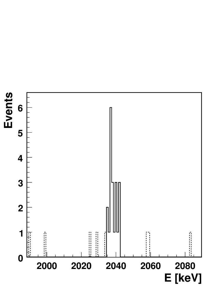
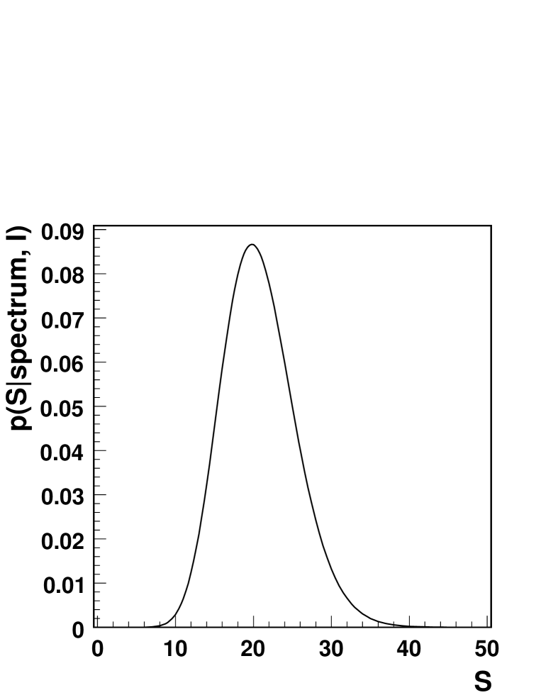
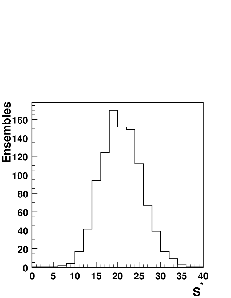
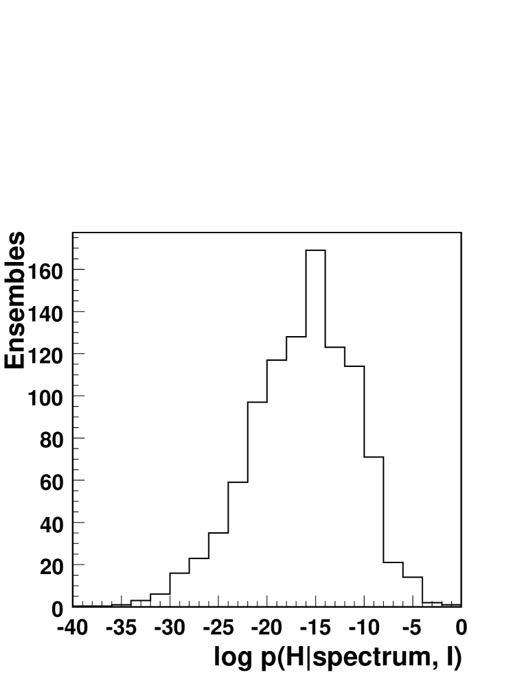
Figure 2: The spectrum (top, left) was randomly generated under the assumptions of a half-life of $2\cdot 10^{25}$ years, a background index of $10^{-3}$ counts/(kg$\cdot$keV$\cdot$y) and an exposure of 100 kg$\cdot$years. The signal events are indicated by a solid line, the background events by a dashed line. The probability density for $S$ (top, right) peaks at $19.8$ which is consistent with the number of signal events, 20, in the spectrum. The distribution of the estimated number of signal events (bottom, left) as well as the distribution of the $\log p(H|\textrm{spectrum})$ (bottom, right) are calculated from ensembles generated under the same assumptions.

In order to simulate the case in which only lower limits on the half-life of the $0\nu\beta\beta$-process are set, ensembles are generated without signal contribution, i.e. $S_{0}=0$. As an example, Fig. 3 (top, left) shows a spectrum from Monte Carlo data generated under the assumptions of a background index of $10^{-3}$ counts/(kg$\cdot$keV$\cdot$y) and an exposure of 100 kg$\cdot$years. No signal events are present in the spectrum.

Figure 3 (top, right) shows the marginalized probability density for $S$, $p(S|\textrm{spectrum})$, for the same spectrum. The mode of $S$ is 0 events.

Figure 3 (bottom, left) shows the distribution of the limit (90% probability) of the signal contribution for 1000 ensembles generated under the same assumptions. The average limit is 3.1.

Figure 3 (bottom, right) shows the distribution of the $p(H|\textrm{spectrum})$ for ensembles generated under the same assumptions. For none of the ensembles could a discovery be claimed.

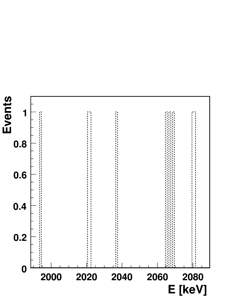
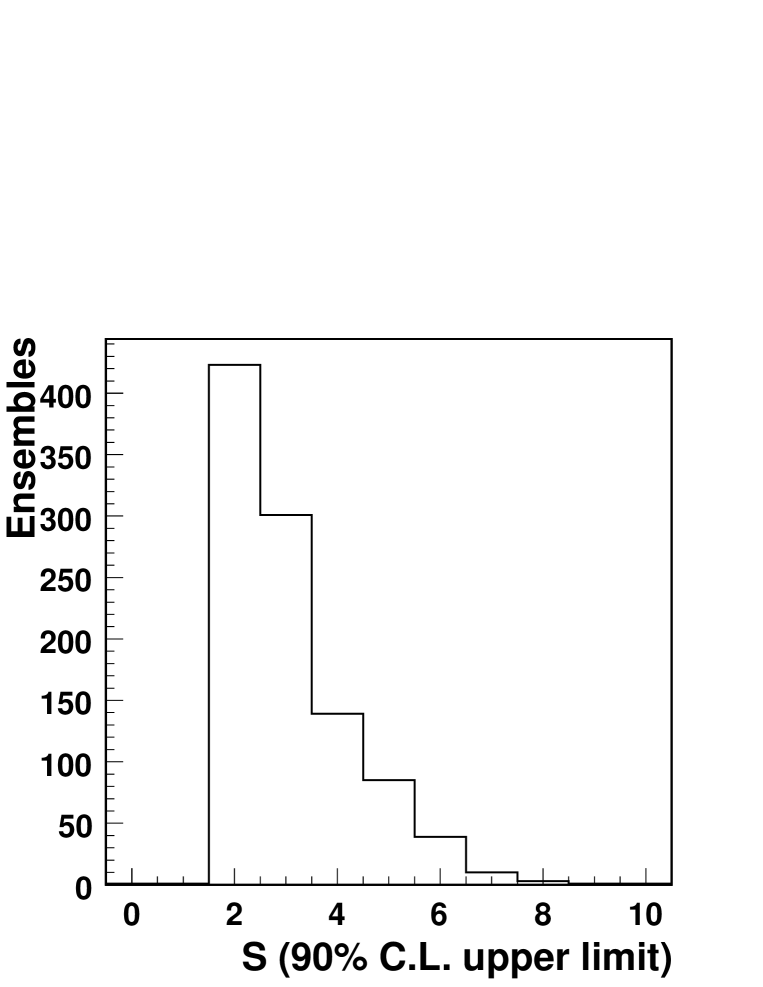
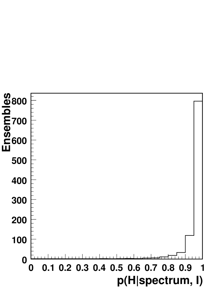
Figure 3: The spectrum (top, left) was randomly generated under the assumptions of a background index of $10^{-3}$ counts/(kg$\cdot$keV$\cdot$y) and an exposure of 100 kg$\cdot$years. No signal events are present in the spectrum. The probability density for $S$ for the same spectrum (top, right) peaks at 0. The distribution of the limit (90% probability) of the signal contribution (bottom, left) as well as the distribution of the $p(H|\textrm{spectrum})$ (bottom, right) are calculated from ensembles generated under the same assumptions.

4.4 Sensitivity

For the ensembles generated without signal contribution the mean of the 90% probability lower limit on the half-life is shown in Figure 4 as a function of the exposure for different background indices. In case no background is present the limit scales linearly with the exposure. With increasing background contribution the limit on the half-life increases more slowly. For the envisioned background index of $10^{-3}$ counts/(kg$\cdot$keV$\cdot$y) and an expected exposure of 100 kg$\cdot$years an average lower limit of $T_{1/2}>13.5\cdot 10^{25}$ years can be set. For the same exposure, the average lower limit is $T_{1/2}>6.0\cdot 10^{25}$ years and $T_{1/2}>18.5\cdot 10^{25}$ years for background indices of $10^{-2}$ counts/(kg$\cdot$keV$\cdot$y) and $10^{-4}$ counts/(kg$\cdot$keV$\cdot$y), respectively.

Using the nuclear matrix elements quoted in [7] the lower limit on the half-life of the $0\nu\beta\beta$-process can be translated into an upper limit on the effective Majorana neutrino mass, $\langle m_{\beta\beta}\rangle$, via

$$\langle m_{\beta\beta}\rangle=(T_{1/2}\cdot G^{0\nu})^{-1/2}\cdot\frac{1}{\langle M^{0\nu}\rangle},$$ (22)

where $G^{0\nu}$ is a phase space factor and $\langle M^{0\nu}\rangle$ is the nuclear matrix element. Figure 4 also shows the expected 90% probability upper limit on the effective Majorana neutrino mass as a function of the exposure. With a background index of $10^{-3}$ counts/(kg$\cdot$keV$\cdot$y) and an exposure of 100 kg$\cdot$years, an upper limit of $\langle m_{\beta\beta}\rangle<200$ meV could be set assuming no $0\nu\beta\beta$-events are observed.

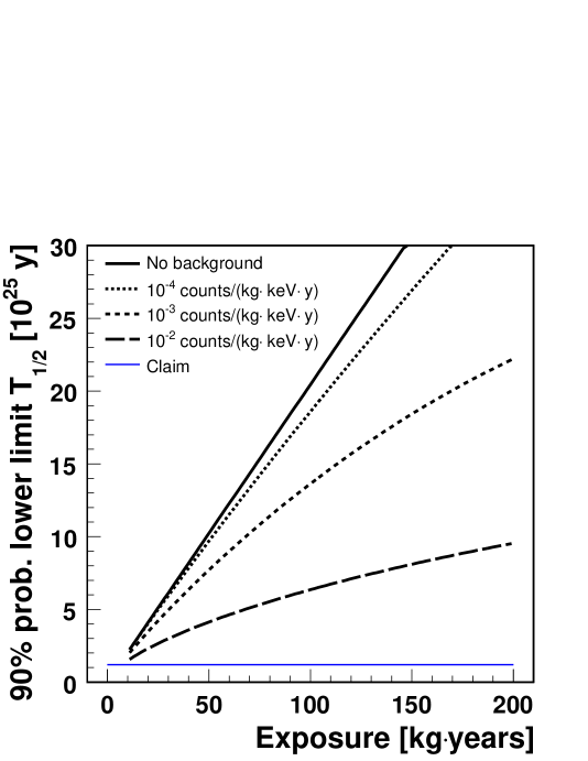
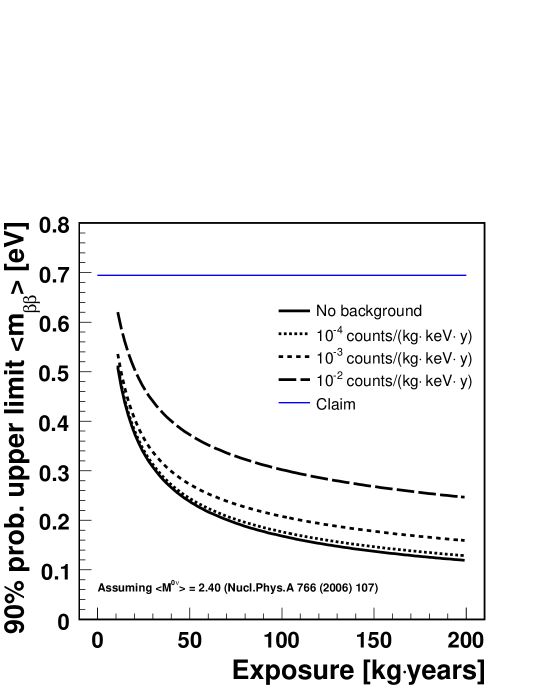
Figure 4: The upper plot shows the expected 90% probability lower limit on the half-life for neutrinoless double beta decay versus the exposure under different background conditions. Also shown is the half-life for the claimed observation [5]. The lower plot shows the expected 90% probability upper limit on the effective Majorana neutrino mass versus the exposure under different background conditions. The effective Majorana neutrino mass for the claimed observation is also shown. All mass values were determined from the half-life using the matrix element reported in [7].

Figure 5 shows the half-life for which 50% of the experiments would report a discovery of neutrinoless double beta decay as a function of the exposure for different background indices. For the envisioned background index of $10^{-3}$ counts/(kg$\cdot$keV$\cdot$y) and an expected exposure of 100 kg$\cdot$years this half-life is $5\cdot 10^{25}$ years.

Using the same matrix elements from reference [7], the half-life is transformed into an effective Majorana neutrino mass. The mass for which 50% of the experiments would report a discovery is shown in Figure 5 (bottom) as a function of the exposure and for different background conditions. For an exposure of 100 kg$\cdot$years and a background index of $10^{-3}$ counts/(kg$\cdot$keV$\cdot$y) neutrinoless double beta decay could be discovered for an effective Majorana neutrino mass of 350 meV (with a 50% probability).

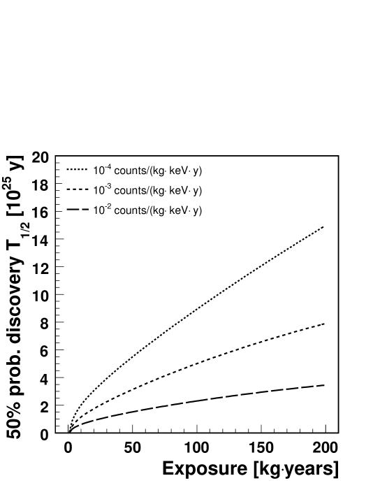
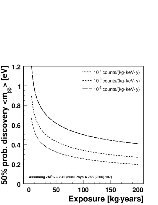
Figure 5: Top: the half-life for which 50% of the experiments would report a discovery, i.e. a probability that the spectrum is due to background processes only, $p(H|\textrm{spectrum})$, of less than 0.01%, is plotted versus the exposure under different background conditions. Bottom: the effective Majorana neutrino mass for which 50% of the experiments would report a discovery versus the exposure under different background conditions. The mass was determined from the half-life using the matrix element reported in [7].

4.5 Influence of the prior probabilities

In order to study the influence of the prior probabilities on the outcome of the experiment, the prior probability for the number of expected signal events, $p_{0}(S)$, was varied. Three different prior probabilities were studied:

• flat prior: $p_{0}(S)\propto const.$ ,

• pessimistic prior: $p_{0}(S)\propto e^{-S/10}$ ,

• peaking prior: $p_{0}(S)\propto e^{1-\tilde{S}/S}/S^{2}$,

where $\tilde{S}$ is the number of events corresponding to a half-life of $1.2\cdot 10^{25}$ years and $S<S_{\mathrm{max}}$. For a background index of $10^{-3}$ counts/(kg keV y) and an exposure of 100 kg years the limit strongly depends on the chosen prior. For the pessimistic prior probability the limit which can be set on the half-life is about 10% higher than that for the flat prior probability. In comparison, the peaking prior gives a 50% lower limit compared to the flat prior. This study makes the role of priors clear. If an opinion is initially strongly held, then substantial data is needed to change it. In the scientific context, consensus priors should be strived for.

5 Conclusions

An analysis method, based on Bayes’ Theorem, was developed which can be used to evaluate the probability that a spectrum can be explained by background processes alone, and thereby determine whether a signal process is necessary. A criterion for claiming evidence for, or discovery of, a signal was proposed. Monte Carlo techniques were described to make predictions about the possible outcomes of the experiments and to evaluate the sensitivity for the process under study.

As an example the method was applied to the case of the GERDA experiment for which the sensitivity to neutrinoless double beta decay of ⁷⁶Ge was calculated. With a background index of $10^{-3}$ counts/(kg$\cdot$keV$\cdot$y) and an exposure of 100 kg$\cdot$years the sensitivity of the half-life of the $0\nu\beta\beta$-process is expected to be $13.5\cdot 10^{25}$ years.

References

- [1] S. Schönert et al. [GERDA Collaboration], Nucl. Phys. Proc. Suppl. 145 (2005) 242.
-
[2]
For an introduction to Bayesian analysis techniques, see e.g.,
’Bayesian Reasoning in Data Analysis’, G. D’Agostini, World Scientific Publishing Company, 2003;
’Data Analysis. A Bayesian Tutorial’, D. S. Sivia, Oxford University Press, USA, 2006;
’Probability Theory - The Logic of Science’, E. T. Jaynes, Cambridge University Press, 2003. - [3] H. V. Klapdor-Kleingrothaus et al., Eur. Phys. J. A 12 (2001) 147 [arXiv:hep-ph/0103062].
- [4] C. E. Aalseth et al. [IGEX Collaboration], Phys. Rev. D 65 (2002) 092007.
- [5] H. V. Klapdor-Kleingrothaus, I. V. Krivosheina, A. Dietz and O. Chkvorets, Phys. Lett. B 586 (2004) 198.
- [6] D. Gonzalez et al., Nucl. Instrum. Meth. A 515 (2003) 634
- [7] V. A. Rodin, A. Faessler, F. Simkovic and P. Vogel, Nucl. Phys. A 766 (2006) 107.