Partial Resonances of Three-Phase Composites at Long Wavelengths

Abstract

We investigate the behaviour of a three-phase composite, structured as a hexagonal array of coated cylinders, when the sum of the dielectric constants of the core and shell equals zero. In such cases, the absorption of the composite is the same as the absorption of a periodic array of solid cylinders of core material and radius equal to the outer radius of the original coated cylinder. When the sum of the dielectric constants of the shell and matrix equals zero, the composite has the same absorption as a periodic array of solid cylinders of core material, and radius exceeding the shell radius.

I Introduction

Previous studies of the effective dielectric constant of a periodic array of coated cylinders, in the quasistatic limit, have revealed some unexpected and interesting results[1, 2, 3]. Specifically, we have used the method of Lord Rayleigh[4] to investigate the analytic properties of the effective dielectric constant of the array, as a function of the core dielectric constant ($\varepsilon_{c}$) and the shell dielectric constant ($\varepsilon_{s}$), while keeping the matrix dielectric constant ($\varepsilon_{m}$) fixed.

We have shown that when $\varepsilon_{c}+\varepsilon_{s}=0$, the composite has exactly the same effective dielectric constant as a periodic array of solid cylinders with dielectric constant $\varepsilon_{c}$ and radius equal to the outer radius of the original coated cylinder. We have also shown that when $\varepsilon_{s}+\varepsilon_{m}=0$, the composite has exactly the same effective dielectric constant as a periodic array of solid cylinders with dielectric constant $\varepsilon_{c}$, and radius exceeding the shell radius. In both cases, the core is magnified and it may be possible for a system with a vanishingly small concentration to exhibit properties like those of a concentrated system. This is what we have called a partially resonant system, since the system has a finite, rather than an infinite, response to the applied field.

The same effect appears in the case of a random mixture of coated cylinders with nonlinear cores and linear shells[5]. Under conditions of partial resonance, the system behaves as a mixture of nonlinear solid cylinders of radii equal to, or larger than, those of the original coated cylinders.

Here, we show how these results carry over to problems of electromagnetic scattering by periodic arrays of coated cylinders, and elucidate the relation between partial resonances and anomalous absorptance of metallic wires [6]. From the many possible ways of packing cylinders in regular arrays in two dimensions we concentrate on the hexagonal lattice that is isotropic for fields applied in the plane perpendicular to the cylinder axes (see Fig. 1). However, the method we use may be applied equally well to any periodic array of coated cylinders.

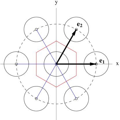
FIG. 1.: The Wigner-Seitz cell (red) with the central inclusion (coated cylinder with $r_{c}=0.03d$, $r_{s}=0.31d$ and $d=1$) and the nearest neighbours (located along the dashed circle) for a hexagonal array. The centers of the nearest neighbours are given by the lattice vectors ${\bf R}_{p}$ for $p\in\{(-1,0),(-1,1),(0,-1),(0,1),(1,-1),(1,0)\}$. We also show the fundamental translation vectors ${\bf e}_{1}=d(1,0)$ and ${\bf e}_{2}=d(1/2,\sqrt{3}/2)$.

Recent work by Pendry et al. [7] has heightened interest in the extraordinary and sometimes paradoxical behaviour which can arise in composite systems, in which one component has a dielectric constant (or a magnetic permeability) which takes approximately a real and negative value. In such a composite we may observe strong focusing of light at a plane interface, or ultra-refraction [8], or a dilute composite masquerading as a concentrated one [1, 2, 3]. Again, the use of metal-coated spheres in photonic crystals has resulted in robust band gaps, independent of sphere-packing geometries [9].

II The Field Identity

A Field Expansions

We consider the electromagnetic modes of a three–phase composite consisting of an array of coated cylinders of infinite length, each aligned parallel to the $z$ axis, inserted into a matrix of dielectric constant $\varepsilon_{m}$ and magnetic permeability $\mu_{m}$. For each cylinder, the core and shell are characterized by the radii $r_{c}$ and $r_{s}$, dielectric constants $\varepsilon_{c}$ and $\varepsilon_{s}$, and magnetic permeabilities $\mu_{c}$ and $\mu_{s}$, respectively. We also assume that the electric and magnetic fields depend on time through a factor $\exp{(-i\omega t)}$. The core and shell of all cylinders, as well as the matrix are homogeneous so that, the fields satisfy the Maxwell equations:

$$\nabla\times{\bf H}= - i\omega\varepsilon({\bf r}){\bf E}~{},~{}~{}\nabla\cdot{\bf E}=0~{},$$ (1)

$$\nabla\times{\bf E}= i\omega\mu({\bf r}){\bf H}~{},~{}~{}\nabla\cdot{\bf H}=0~{},$$ (2)

with

$$\varepsilon({\bf r})=\left\{\begin{array}[]{lcl}\varepsilon_{m}&~{}~{}{\rm for{}{}}&{\bf r}\in\Omega_{m}\,,\\ \varepsilon_{s}&~{}~{}{\rm for{}{}}&{\bf r}\in\Omega_{s}\,,\\ \varepsilon_{c}&~{}~{}{\rm for{}{}}&{\bf r}\in\Omega_{c}\,,\\ \end{array}\right.$$ (3)

and

$$\mu({\bf r})=\left\{\begin{array}[]{lcl}\mu_{m}&~{}~{}{\rm for{}{}}&{\bf r}\in\Omega_{m}\,,\\ \mu_{s}&~{}~{}{\rm for{}{}}&{\bf r}\in\Omega_{s}\,,\\ \mu_{c}&~{}~{}{\rm for{}{}}&{\bf r}\in\Omega_{c}\,.\\ \end{array}\right.$$ (4)

Here, in the $xy-$plane, $\Omega_{c}$ denotes the union of all the domains occupied by cylinder cores, while $\Omega_{s}$ denotes the union of all the domains occupied by the cylinder shells. Thus, $\Omega_{c}\bigcup\Omega_{s}$ represents the region occupied by all the cylinders in the array and $\Omega_{m}$ is the region between the cylinders (the matrix region).

By eliminating ${\bf E}$ or ${\bf H}$ between (1) and (2), we obtain the Helmholtz equations for the components of the fields:

$$\left(\nabla^{2}+\kappa^{2}\right)\left\{\begin{array}[]{c}{\bf E}\\ {\bf H}\end{array}\right\}=0\,,$$ (5)

where $\kappa^{2}=\omega^{2}\varepsilon\mu$ is again a function of position. The axes of the cylinders in the array are parallel to the $z-$axis, and the fields are taken to depend on $z$ through the factor $\exp(i\beta z)$, with $\beta$ representing the propagation constant along the $z$ direction, in all the regions $\Omega_{c}$, $\Omega_{s}$ and $\Omega_{m}$. Also, in cylindrical coordinates ($r$, $\theta$, $z$), the field components $E_{z}$ and $H_{z}$ determine the other four field components through the relations[10]:

$$E_{r} = \frac{i}{\kappa^{2}-\beta^{2}}\left[\beta\,\frac{\partial E_{z}}{\partial r}+\frac{\omega\mu}{r}\,\frac{\partial H_{z}}{\partial\theta}\right]\,,$$ (6)

$$E_{\theta} = \frac{i}{\kappa^{2}-\beta^{2}}\left[\frac{\beta}{r}\,\frac{\partial E_{z}}{\partial\theta}-\omega\mu\,\frac{\partial H_{z}}{\partial r}\right]\,,$$ (7)

$$H_{r} = \frac{-i}{\kappa^{2}-\beta^{2}}\left[\frac{\omega\varepsilon}{r}\,\frac{\partial E_{z}}{\partial\theta}-\beta\,\frac{\partial H_{z}}{\partial r}\right]\,,$$ (8)

$$H_{\theta} = \frac{i}{\kappa^{2}-\beta^{2}}\left[\omega\varepsilon\,\frac{\partial E_{z}}{\partial r}+\frac{\beta}{r}\,\frac{\partial H_{z}}{\partial\theta}\right]\,.$$ (9)

The field components $E_{z}$ and $H_{z}$ satisfy the Helmholtz equations:

$$\left(\nabla_{\perp}^{2}+k^{2}\right)\left\{\begin{array}[]{c}E_{z}\\ H_{z}\end{array}\right\}=0\,,$$ (10)

where $\nabla_{\perp}^{2}$ is the transverse Laplacian and

$$k^{2}=\kappa^{2}-\beta^{2}\,,$$ (11)

represents the transverse (in-plane) propagation constant.

For the cylinder centered at the origin of coordinates, we represent the electric and magnetic fields $E_{z}$ and $H_{z}$ (denoted here by $V$), by series expansions in terms of cylindrical harmonics:

$$V(r,\theta)=\left\{\begin{array}[]{l}{\displaystyle\sum_{l=-\infty}^{\infty}A_{l}^{c}J_{l}(k_{c}r)\,e^{il\theta}}\,,\\ {\displaystyle\sum_{l=-\infty}^{\infty}\left[A_{l}^{s}J_{l}(k_{s}r)+B_{l}^{s}Y_{l}(k_{s}r)\right]e^{il\theta}}\,,\\ {\displaystyle\sum_{l=-\infty}^{\infty}\left[A_{l}^{m}J_{l}(k_{m}r)+B_{l}^{m}Y_{l}(k_{m}r)\right]e^{il\theta}}\,,\end{array}\right.$$ (12)

where $J$ and $Y$ represent the Bessel functions of the first and second kind. The three forms of the series expansions in (12) correspond to $0\leq r\leq r_{c}$ (i.e., inside the core), $r_{c}\leq r\leq r_{s}$ (i.e., inside the shell) and $r\geq r_{s}$ (i.e., in the matrix), respectively. Also, the superscripts $c$, $s$ and $m$ label the fields inside the cylinder core, cylinder shell, and in the matrix, respectively. Thus, we have $k_{c}^{2}=\omega^{2}\varepsilon_{c}\mu_{c}$, $k_{s}^{2}=\omega^{2}\varepsilon_{s}\mu_{s}$, and $k_{m}^{2}=\omega^{2}\varepsilon_{m}\mu_{m}$.

B Boundary Conditions

The boundary conditions express the continuity of the tangential components of the electric ($E_{z}$, $E_{\theta}$) and magnetic ($H_{z}$ and $H_{\theta}$) fields across the core and shell surfaces. When the crystal momentum is perpendicular to the axes of the cylinders in the array, we have $\beta=0$, and the problem can be reduced to solving two independent problems[11]: (i) for TM or $s$ polarization (when $H_{z}=0$ and the transverse parts of ${\bf E}$ and ${\bf H}$ are generated by $\nabla_{\perp}E_{z}$), and (ii) for TE or $p$ polarization (when $E_{z}=0$ and $\nabla_{\perp}H_{z}$ gives the transverse components of ${\bf E}$ and ${\bf H}$). Thus, depending on the polarization, we obtain:

$$\left.E_{z}^{(c)}\right|_{r=r_{c}} = \left.E_{z}^{(s)}\right|_{r=r_{c}},$$ (13)

$$\left.\frac{1}{\mu_{c}}\,\frac{\partial E_{z}^{(c)}}{\partial r}\right|_{r=r_{c}} = \left.\frac{1}{\mu_{s}}\,\frac{\partial E_{z}^{(s)}}{\partial r}\right|_{r=r_{c}},$$ (14)

$$\left.E_{z}^{(s)}\right|_{r=r_{s}} = \left.E_{z}^{(m)}\right|_{r=r_{s}},$$ (15)

$$\left.\frac{1}{\mu_{s}}\,\frac{\partial E_{z}^{(s)}}{\partial r}\right|_{r=r_{s}} = \left.\frac{1}{\mu_{m}}\,\frac{\partial E_{z}^{(m)}}{\partial r}\right|_{r=r_{s}},$$ (16)

for TM polarization, and:

$$\left.H_{z}^{(c)}\right|_{r=r_{c}} = \left.H_{z}^{(s)}\right|_{r=r_{c}},$$ (17)

$$\left.\frac{1}{\varepsilon_{c}}\,\frac{\partial H_{z}^{(c)}}{\partial r}\right|_{r=r_{c}} = \left.\frac{1}{\varepsilon_{s}}\,\frac{\partial H_{z}^{(s)}}{\partial r}\right|_{r=r_{c}},$$ (18)

$$\left.H_{z}^{(s)}\right|_{r=r_{s}} = \left.H_{z}^{(m)}\right|_{r=r_{s}},$$ (19)

$$\left.\frac{1}{\varepsilon_{s}}\,\frac{\partial H_{z}^{(s)}}{\partial r}\right|_{r=r_{s}} = \left.\frac{1}{\varepsilon_{m}}\,\frac{\partial H_{z}^{(m)}}{\partial r}\right|_{r=r_{s}},$$ (20)

for TE polarization.

In the case of TM polarization, for the cylinder centered at the origin of coordinates, we use the series expansions (12) for $E_{z}$, and by means of the boundary conditions (13-16) we obtain relations of the form:

$$\left[\begin{array}[]{c}A_{l}^{m}\\ B_{l}^{m}\end{array}\right] = \left[\begin{array}[]{rr}J_{l}(k_{m}r_{s})&Y_{l}(k_{m}r_{s})\\ Z_{m}^{-1}J_{l}^{\prime}(k_{m}r_{s})&Z_{m}^{-1}Y_{l}^{\prime}(k_{m}r_{s})\end{array}\right]^{-1}$$ (25)

$$\times \left[\begin{array}[]{rr}J_{l}(k_{s}r_{s})&Y_{l}(k_{s}r_{s})\\ Z_{s}^{-1}J_{l}^{\prime}(k_{s}r_{s})&Z_{s}^{-1}Y_{l}^{\prime}(k_{s}r_{s})\end{array}\right]$$ (28)

$$\times \left[\begin{array}[]{rr}J_{l}(k_{s}r_{c})&Y_{l}(k_{s}r_{c})\\ Z_{s}^{-1}J_{l}^{\prime}(k_{s}r_{c})&Z_{s}^{-1}Y_{l}^{\prime}(k_{s}r_{c})\end{array}\right]^{-1}$$ (31)

$$\times \left[\begin{array}[]{rr}J_{l}(k_{c}r_{c})&Y_{l}(k_{c}r_{c})\\ Z_{c}^{-1}J_{l}^{\prime}(k_{c}r_{c})&Z_{c}^{-1}Y_{l}^{\prime}(k_{c}r_{c})\end{array}\right]\left[\begin{array}[]{c}A_{l}^{c}\\ 0\end{array}\right]\,,$$ (36)

or

$$A_{l}^{m}=-M_{l}B_{l}^{m}\,.$$ (37)

In (28), the prime indicates the derivative of the corresponding function and $Z_{i}=\sqrt{\mu_{i}/\varepsilon_{i}}$ ($i=m,s,c$) represent the impedances of the matrix, shell and core, respectively. For TE polarization we obtain the relation between $A_{l}^{m}$ and $B_{l}^{m}$ by changing $Z_{i}\rightarrow 1/Z_{i}$ in (28).

The structure of (28) allows us a generalization to multicoated cylinders, and for this reason we have added the second column in the last matrix. However, this last matrix is multiplied by the vector $[A_{l}^{c},0]^{T}$ corresponding to the field expansion inside the core (i.e., the first form in (12)). Note that the first two matrices in the right side of (28) arise from the boundary conditions at the interface between the shell and matrix ((15) and (16)), while the next two matrices come from the boundary conditions at the core – shell interface ((13) and (14)). Consequently, in the case of a multicoated cylinder, we may infer the form of a general term representing the interface $i$ (between the $i^{\rm th}$ and $(i+1)^{\rm th}$ media) characterized by the radius $r_{i}$:

$${\bf M}_{l}^{i,i+1} = \left[\begin{array}[]{rr}J_{l}(k_{i}r_{i})&Y_{l}(k_{i}r_{i})\\ Z_{i}^{-1}J_{l}^{\prime}(k_{i}r_{i})&Z_{i}^{-1}Y_{l}^{\prime}(k_{i}r_{i})\end{array}\right]^{-1}$$ (40)

$$\times \left[\begin{array}[]{rr}J_{l}(k_{i+1}r_{i})&Y_{l}(k_{i+1}r_{i})\\ Z_{i+1}^{-1}J_{l}^{\prime}(k_{i+1}r_{i})&Z_{i+1}^{-1}Y_{l}^{\prime}(k_{i+1}r_{i})\end{array}\right].$$ (43)

Here, we have counted the layers from the exterior to interior and thus, for $n-1$ shells, the matrix is indexed by $i=0$ and the core (the innermost medium) by $i=n$. Now, Eq. (28) takes the form

$$\left[\begin{array}[]{c}A_{l}^{0}\\ B_{l}^{0}\end{array}\right]=\left(\prod_{i=0}^{n-1}{\bf M}_{l}^{i,i+1}\right)\left[\begin{array}[]{c}A_{l}^{n+1}\\ 0\end{array}\right]\,.$$ (44)

We also obtain the expression for the TE polarization by substituting $Z_{i}\rightarrow 1/Z_{i}$.

C The Generalized Rayleigh Identity

For each polarization (TM or TE), we may write a Generalized Rayleigh Identity of the form[12, 13]:

$$M_{l}B_{l}+\sum_{n=-\infty}^{\infty}S_{l-n}^{Y}(k_{m},{\bf k}_{0})\,B_{n}=0\,,$$ (45)

with $M_{l}$ from (37) and $-\infty<l<\infty$. The quantities $S_{l}^{Y}$ are dynamic lattice sums, which may be evaluated using accelerated summation over the reciprocal array[12]:

$$S_{l}^{Y}(k_{m},{\bf k}_{0})J_{l+n}(k_{m}\xi)=$$ (46)

$$-\left[Y_{n}(k_{m}\xi)+\frac{1}{\pi}\sum_{q=1}^{n}\frac{(n-q)!}{(q-1)!}\left(\frac{2}{k_{m}\xi}\right)^{n-2q+2}\right]\delta_{l,0}$$ (47)

$$-i^{l}\frac{4}{A}\sum_{h}\left(\frac{k_{m}}{Q_{h}}\right)^{n}\frac{J_{l+n}(Q_{h}\xi)}{Q_{h}^{2}-k_{m}^{2}}e^{il\theta_{h}}.$$ (48)

Here, $n$ is an arbitrary non–negative integer, $\xi$ is the length of an arbitrary vector inside the unit cell (shorter than the shortest line connecting two of its vertices), and $A$ represents the area of the unit cell. The vector ${\bf k}_{0}$ is the in–plane component of the “crystal momentum” ${\bf k}_{B}={\bf k}_{0}+\beta{\bf{\widehat{z}}}$, with ${\bf{\widehat{z}}}$ the unit vector along the $z-$axis. Note that, in this paper we consider only the case $\beta=0$, so that ${\bf k}_{B}={\bf k}_{0}$.

The quantities ${\bf Q}_{h}$ and $\theta_{h}$ from (48) depend on the type of the array. In our case, the hexagonal array is defined by the fundamental translation vectors ${\bf e}_{1}=d(1,0)$ and ${\bf e}_{2}=d(1/2,\sqrt{3}/2)$, where $d$ is the array constant (see Fig. 1). Hence, the centers of the cylinders are located at the points given by the radius vectors

$${\bf R}_{p}=p_{1}{\bf e}_{1}+p_{2}{\bf e}_{2},$$ (49)

with $p$ denoting the pair of integers $(p_{1},p_{2})\in{\mathbb{Z}}^{2}$. The fundamental vectors of the reciprocal array are given by the relations

$${\bf u}_{1} = \frac{2\pi}{A}{\bf e}_{2}\times{\bf e}_{3}=\frac{2\pi}{d}\left(1,-\frac{1}{\sqrt{3}}\right),$$ (50)

$${\bf u}_{2} = \frac{2\pi}{A}{\bf e}_{3}\times{\bf e}_{1}=\frac{2\pi}{d}\left(0,\frac{2}{\sqrt{3}}\right),$$ (51)

where $A=\|{\bf e}_{1}\times{\bf e}_{2}\|$ and ${\bf e}_{3}=({\bf e}_{1}\times{\bf e}_{2})/A$ is a dimensionless unit vector, along the $z$ axis. With the vectors (50) and (51) we form the reciprocal lattice vectors

$${\bf K}_{h}=h_{1}{\bf u}_{1}+h_{2}{\bf u}_{2},$$ (52)

where $h=(h_{1},h_{2})\in{\mathbb{Z}}^{2}$. Finally, we have ${\bf Q}_{h}={\bf k}_{0}+{\bf K}_{h}$ and $\theta_{h}=\arg{({\bf Q_{h}})}$.

The eigenfrequencies ($\omega$) of the Helmholtz equation (5) are obtained from the zeros of the determinant of (45). In the coordinate system $\omega$ versus ${\bf k}_{B}$, the photonic band diagrams are given by the trajectories of the eigenfrequencies $\omega$ when ${\bf k}_{B}$ follows the boundary of one of the irreducible regions in the first Brillouin zone (see Fig. 2).

In the case of metallic media, ${\bf k}_{B}$ becomes complex. It is then simpler to use a summation method [14] different from (48), and a technique, based on Bloch’s theorem, developed originally by McRae[15] in low energy electron diffraction, and applied recently to photonic crystals by Gralak et al. [8]. We consider the array as an infinite stack of gratings and calculate the scattering matrices for a single grating in the array [16]. Then, the complex crystal momentum ${\bf k}_{B}$ is found by solving an eigenvalue problem [17].

III The Long Wavelength Limit

A Partial Resonances

The solution of the problem of electromagnetic scattering by a solid cylinder, at normal incidence and in the long wavelength limit[18], revealed the occurrence of a resonance in scattering when the relative dielectric constant of the cylinder was -1. Later, the existence of this resonance was proved experimentally in studies of radio reflection by meteor trails[19], and of plasma columns[20, 21]. Also, Wait[22, 23] has shown that in the long wavelength limit the scattering resonances given by the formula

$$\left(\mu_{1}+\mu_{2}\right)\left(\varepsilon_{1}+\varepsilon_{2}\right)=0,$$ (53)

where the label 1 refers to the cylinder and 2 refers to the homogeneous medium outside the cylinder, are independent of the polarization and angle of incidence. Note that, in electrostatics the condition $(\varepsilon_{1}+\varepsilon_{2})=0$ defines the accumulation point for the poles and zeros of the effective dielectric constant of a two–phase composite[24, 25], with $(\mu_{1}+\mu_{2})=0$ corresponding to magnetostatics.

We applied the method developed by Wait[22] to solve the problem of scattering of a plane wave by a coated cylinder at oblique incidence. In this case, in the long wavelength limit we obtained the resonance condition

$$\left(\mu_{c}+\mu_{s}\right)\left(\mu_{s}+\mu_{m}\right)\left(\varepsilon_{c}+\varepsilon_{s}\right)\left(\varepsilon_{s}+\varepsilon_{m}\right)=0,$$ (54)

which describes precisely the electrostatic partial resonances of a three–phase composite[1, 2, 3], plus their magnetostatic counterpart. The resonance condition (54) also suggests a generalization to a $n$–phase composite, of the form

$$\prod_{i=0}^{n-1}\left(\mu_{i}+\mu_{i+1}\right)\left(\varepsilon_{i}+\varepsilon_{i+1}\right)=0,$$ (55)

for the case of a multi-coated cylinder. Here, $\mu_{n}$ and $\varepsilon_{n}$ denote the magnetic permeability and dielectric constant of the innermost phase (core), while $\mu_{0}$ and $\varepsilon_{0}$ represent the magnetic permeability and dielectric constant of the medium outside the composite.

B TE Polarization

We concentrate now on non-magnetic materials for which $\mu_{m}=\mu_{s}=\mu_{c}=\mu_{0}$, so that $\varepsilon_{m}=n_{m}^{2}\varepsilon_{0}$, $\varepsilon_{s}=n_{s}^{2}\varepsilon_{0}$ and $\varepsilon_{c}=n_{c}^{2}\varepsilon_{0}$, where $\varepsilon_{0}$ is the dielectric constant of free space, and $n_{i}$ ($i=m,s,c$) represent the refractive indexes of the matrix, shell and core, respectively. In the long wavelength limit ($k_{m}\rightarrow 0$), we use the expressions of the Bessel functions for small arguments[26] in the boundary conditions coefficients $M_{l}$ from (37), for TE polarization. For $l\neq 0$ we obtain

$$M_{l}=M_{-l}=-\frac{1}{\pi}\left(\frac{2}{k_{m}r_{s}}\right)^{2l}l!(l-1)!\,\gamma_{l}\,,$$ (56)

where

$$\gamma_{l}=\frac{r_{c}^{2l}(\varepsilon_{s}-\varepsilon_{c})(\varepsilon_{m}-\varepsilon_{s})+r_{s}^{2l}(\varepsilon_{s}+\varepsilon_{c})(\varepsilon_{m}+\varepsilon_{s})}{r_{c}^{2l}(\varepsilon_{s}-\varepsilon_{c})(\varepsilon_{m}+\varepsilon_{s})+r_{s}^{2l}(\varepsilon_{s}+\varepsilon_{c})(\varepsilon_{m}-\varepsilon_{s})}\,,$$ (57)

while for $l=0$, we obtain a completely different form

$$M_{0}=-\frac{1}{\pi}\left(\frac{2}{k_{m}r_{s}}\right)^{4}\frac{\varepsilon_{m}}{(\varepsilon_{s}-\varepsilon_{c})(r_{c}/r_{s})^{4}+(\varepsilon_{m}-\varepsilon_{s})}\,.$$ (58)

To relate the long wavelength limit of the dynamic problem with the corresponding problem in electrostatics we apply the same method as in Ref. [27]. Thus, the boundary conditions (17-20) correspond to an electrostatic problem in which the inverse of the dielectric constants ($\varepsilon_{c}\rightarrow 1/\varepsilon_{c}$, $\varepsilon_{s}\rightarrow 1/\varepsilon_{s}$ and $\varepsilon_{m}\rightarrow 1/\varepsilon_{m}$) have to be considered. This will also change $\gamma_{l}\rightarrow-\gamma_{l}$. Now, the boundary conditions (37) for $l\neq 0$ can be written in the form

$$A_{l}^{m}=-\frac{1}{\pi}\left(\frac{2}{k_{m}}\right)^{2l}l!(l-1)!\,\gamma_{l}\,\frac{B_{l}^{m}}{r_{s}^{2l}}.$$ (59)

In electrostatics, the corresponding relationship between the coefficients $A_{l}$ and $B_{l}$ which controls the response of a coated cylinder to an external field, has the form[1]

$$A_{l}^{\prime}=\gamma_{l}\,\frac{B_{l}^{\prime}}{r_{s}^{2l}}\,.$$ (60)

Note that, due to the symmetry properties of the electrostatic potential, $l$ cannot take even values in the case of a square array, or values which are multiples of 3 in the case of a hexagonal array[28]. By comparing (59) with (60) we may deduce the relation between static and dynamic multipole coefficients

$$B_{l}^{\prime}=-\frac{1}{\pi}\left(\frac{2}{k_{m}}\right)^{2l}l!(l-1)!\,B_{l}^{m}\,.$$ (61)

for $l\neq 0$. The dynamic field in the matrix ($H_{z}^{(m)}$) may be approximated by[27, 29]

$$H_{z}^{(m)}({\bf r})=A_{0}\exp{[ik_{B}V_{m}({\bf r})]}+{\mathcal{O}}(k_{B}^{2})\,,$$ (62)

where $V_{m}$ is the solution of the static problem. Note that the derivation of (62) does not involve the boundary conditions coefficient $M_{0}$ from (58).

In electrostatics, the partial resonances of a three–phase composite consisting of coated cylinders are defined by the equations

$$\varepsilon_{c}+\varepsilon_{s} = 0\qquad({\rm core--shell~{}resonance}),$$ (63)

$$\varepsilon_{s}+\varepsilon_{m} = 0\qquad({\rm shell--matrix~{}resonance}),$$ (64)

when (60) becomes

$$A_{l}^{\prime}=\frac{\varepsilon_{m}+\varepsilon_{c}}{\varepsilon_{m}-\varepsilon_{c}}\,\frac{B_{l}^{\prime}}{r_{s}^{2l}}\,,$$ (65)

or

$$A_{l}^{\prime}=\frac{\varepsilon_{m}+\varepsilon_{c}}{\varepsilon_{m}-\varepsilon_{c}}\,\frac{B_{l}^{\prime}}{(r_{s}^{2}/r_{c})^{2l}}\,,$$ (66)

respectively. In the first case, the field inside the coated cylinder is exactly the same as would be found within a solid cylinder of radius $r_{s}$ and dielectric constant $\varepsilon_{c}$, while the potential outside the coated cylinder, in the matrix, is precisely the same as that outside the solid cylinder[1]. The second case corresponds to an effective dielectric constant of the array of coated cylinders, identical with that of an array of solid cylinders of radius $r_{s}^{2}/r_{c}>r_{s}$ (the geometrical image of the core boundary with respect to the shell outer boundary), and dielectric constant $\varepsilon_{c}$. Now, the field external to the coated cylinder and beyond the radius $r_{s}^{2}/r_{c}$ is the same as that external to the solid cylinder[1].

Since it is the relationship between the coefficients $A_{l}$ and $B_{l}$ which controls the response of a coated cylinder to an external field, equations (60) and (59) show that this response is determined by $\gamma_{l}$ in electrostatics as well as in the long wavelengths limit of electrodynamics. The limiting process is smooth and, therefore, we expect a resonant behaviour of the array of coated cylinders, for nonzero frequencies, when one of the conditions (63) or (64) is satisfied.

C TM Polarization

The behaviour of the array of coated cylinders is completely different in the case of TM polarization. Now, in the long wavelength limit, the boundary conditions coefficients $M_{l}$ from (37) take the form

$$M_{l}=M_{-l}$$ (67)

$$=\frac{1}{\pi}\left(\frac{2}{k_{m}r_{s}}\right)^{2l+2}\frac{2\,l!(l+1)!\,\varepsilon_{m}}{(\varepsilon_{c}-\varepsilon_{s})(r_{c}/r_{s})^{2l+2}+(\varepsilon_{s}-\varepsilon_{m})},$$ (68)

for $l\neq 0$, and

$$M_{0}=\frac{1}{\pi}\left(\frac{2}{k_{m}r_{s}}\right)^{2}\frac{\varepsilon_{m}}{(\varepsilon_{c}-\varepsilon_{s})(r_{c}/r_{s})^{2}+(\varepsilon_{s}-\varepsilon_{m})}\,.$$ (69)

Following the same method as in Ref.[27] we consider the central equation ($l=0$) of the Rayleigh identity (45)

$$\left[M_{0}+S_{0}^{Y}(k_{m},{\bf k}_{0})\right]B_{0}+\sum_{n\neq 0}S_{-n}^{Y}(k_{m},{\bf k}_{0})B_{n}=0\,,$$ (70)

and employ the forms of lattice sums for small $k_{m}$[27]

$$S_{0}^{Y} \sim \frac{4}{Ak_{0}^{2}(\alpha^{2}-1)}\,,$$ (71)

$$S_{1}^{Y} \sim \frac{4i}{Ak_{0}^{2}\alpha(\alpha^{2}-1)}\,e^{i\theta_{0}}\,,$$ (72)

$$S_{n}^{Y} \sim {\mathcal{O}}(k_{0}^{-n})\,,\quad{\rm for}~{}l\geq 2\,,\quad\left(S_{-n}^{Y}=\overline{S_{n}^{Y}}\right),$$ (73)

where the superposed bar denotes complex conjugation, $A$ is the area of the Wigner-Seitz cell, $\theta_{0}=\arg{({\bf k}_{0})}$ and $\alpha=k_{m}/k_{0}$. We also introduce the relations between dynamic ($B_{n}$) and static ($B_{n}^{\prime}$) multipole coefficients[27]

$$B_{n} \sim (k_{m}r_{s})^{n+2}\,B_{n}^{\prime}\,,$$ (74)

$$B_{-n} \sim (k_{m}r_{s})^{n+2}\,\overline{B_{n}^{\prime}}\,,$$ (75)

for $n\geq 0$. Here, the static multipole coefficients are, to leading order, independent of $k_{m}$. Finally, the equation (70) becomes

$$\left[\frac{\varepsilon_{m}}{(\varepsilon_{c}-\varepsilon_{s})(r_{c}/r_{s})^{2}+(\varepsilon_{s}-\varepsilon_{m})}-\frac{\pi\alpha^{2}r_{s}^{2}}{A(1-\alpha^{2})}\right]B_{0}^{\prime}$$ (76)

$$+\sum_{n\neq 0}B_{n}^{\prime}\,{\mathcal{O}}(k_{m})=0.$$ (77)

From all the other equations ($l\neq 0$) of (45) we obtain $B_{l}^{\prime}=0$ so that, in the long wavelengths limit, to leading order, the only non-trivial solution of the Rayleigh identity (45) is $B_{0}^{\prime}\neq 0$ and $B_{n}^{\prime}=0$ ($\forall n\neq 0$), if

$$\frac{\varepsilon_{m}}{\alpha^{2}}=f_{c}\varepsilon_{c}+f_{s}\varepsilon_{s}+f_{m}\varepsilon_{m}\,,$$ (78)

with $f_{c}=\pi r_{c}^{2}/A$, $f_{s}=\pi(r_{s}^{2}-r_{c}^{2})/A$ and $f_{m}=1-\pi r_{s}^{2}/A$, denoting the area fractions of the phases inside the unit cell. From (12) we derive the form of the electric field in the matrix:

$$E_{z}^{(m)}\sim\frac{\varepsilon_{m}}{(\varepsilon_{c}-\varepsilon_{s})(r_{c}/r_{s})^{2}+(\varepsilon_{s}-\varepsilon_{m})}B_{0}^{\prime}\,.$$ (79)

Equation (78) represents the linear mixing formula [30] for the effective dielectric constant of an array of coated cylinders subject to a uniform field applied along the cylinder axis. Note that there are no terms of the form $\varepsilon_{c}+\varepsilon_{s}$ or $\varepsilon_{s}+\varepsilon_{m}$ in (77) or (78) to indicate a core–shell or shell–matrix partial resonance. Again, the limiting process is smooth and, consequently, we do not expect a resonant behaviour of the array of coated cylinders, for any frequency, in the case of TM polarization.

IV Numerical Results

In this section we discuss the behaviour of a three–phase composite consisting of aluminium oxide (${\rm Al}_{2}{\rm O}_{3}$), whose refractive index depends on the frequency, and two pure dielectric phases: one with a refractive index $n_{d}=1.37$, and vacuum ($n_{0}=1$).

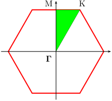
FIG. 2.: The irreducible part (green triangle) of the first Brillouin zone.

Note that, all the defining equations for partial resonances and the boundary conditions coefficients, in the long wavelengths limit or in electrostatics, are homogeneous functions of dielectric constants. Also, note that the phases are non–magnetic materials. Hence, in this section we will denote by $\varepsilon$ the relative dielectric constant $\varepsilon/\varepsilon_{0}=n^{2}$ (the square of the refractive index). With this notation, we use the experimental data for the real and imaginary parts of the refractive index of aluminium oxide in the region $0.3\mu{\rm m}\leq\lambda\leq 20.0\mu{\rm m}$[31], to evaluate the relative dielectric constant of aluminium oxide ($\varepsilon_{\mbox{${\rm Al}_{2}{\rm O}_{3}$}}=n_{\mbox{${\rm Al}_{2}{\rm O}_{3}$}}^{2}$). Also, the relative dielectric constant of the second phase is $\varepsilon_{d}=1.876$.

We assume that the composite is structured as a hexagonal array (array constant $d$=1$\mu$m) of coated cylinders (core radius $r_{c}=0.03\mu$m, cylinder radius (core+coating) $r_{s}=0.31\mu$m) in vacuum. The Wigner–Seitz cell is shown in Fig. 1, while the irreducible part of the first Brillouin zone (K$\Gamma$MK) is shown Fig. 2. For this region of the first Brillouin zone, the coordinates of the corners are

$${\rm K}\left(\frac{2\pi}{3d},\frac{2\pi}{d\sqrt{3}}\right),\quad\Gamma(0,0),\quad{\rm M}\left(0,\frac{2\pi}{d\sqrt{3}}\right).$$

A Partial Resonances

In the case of an absorbing (metallic–type) core and a dielectric shell, the constant, the positive value of the shell dielectric constant ($\varepsilon_{s}=n_{d}^{2}$) makes impossible a relation of the type $n_{d}^{2}+n_{m}^{2}=0$ corresponding to a shell–matrix partial resonance. Hence, we expect only core–shell partial resonances, which are defined by the equation

$$n_{\mbox{${\rm Al}_{2}{\rm O}_{3}$}}^{2}+n_{d}^{2}=0\,.$$ (80)

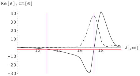
FIG. 3.: Real (solid curve) and imaginary (dashed curve) part of ${\rm Al}_{2}{\rm O}_{3}$ relative dielectric constant versus wavelength. The horizontal red line shows $-n_{d}^{2}$, while the vertical magenta lines mark the two solutions $\lambda_{1}$ and $\lambda_{2}$, of (81).

Note that, $n_{d}^{2}$ is real and so we will solve the real part of (80):

$$\Re e\left(n_{\mbox{${\rm Al}_{2}{\rm O}_{3}$}}^{2}+n_{d}^{2}\right)=0\,,$$ (81)

and then check the magnitude of the imaginary part.

In the wavelengths domain $0.3\mu{\rm m}\leq\lambda\leq 20.0\mu{\rm m}$, Eq. (81) has two solutions

$$\lambda_{1}\approx 12.861\mu{\rm m},$$ (82)

giving a value of

$$n_{\mbox{${\rm Al}_{2}{\rm O}_{3}$}}^{2}+n_{d}^{2}\approx 10^{-5}+0.329\,i\,,$$ (83)

when substituted in (80), and

$$\lambda_{2}\approx 17.333\mu{\rm m},$$ (84)

giving a value of

$$n_{\mbox{${\rm Al}_{2}{\rm O}_{3}$}}^{2}+n_{d}^{2}\approx 10^{-4}+32.72\,i\,,$$ (85)

when substituted in (80). They are marked by the magenta vertical lines in Fig. 3. Actually, the magnitude of the imaginary part of (80) shows that we may have a partial core–shell resonance at $\lambda_{1}$, while the second root appears only as the result of an anomaly of $n_{\mbox{${\rm Al}_{2}{\rm O}_{3}$}}^{2}$ around $\lambda_{2}$.

In the case of dielectric core and absorbing (metallic–type) shell we expect the coated cylinders to exhibit both types of partial resonances: core–shell

$$n_{d}^{2}+n_{\mbox{${\rm Al}_{2}{\rm O}_{3}$}}^{2}=0$$

and shell–matrix

$$n_{\mbox{${\rm Al}_{2}{\rm O}_{3}$}}^{2}+n_{m}^{2}=0.$$

The wavelengths at which the first type of partial resonances occurs are given by Eq. (81), while the second type, is identical with the classical resonance[24, 25] exhibited by solid cylinders from ${\rm Al}_{2}{\rm O}_{3}$ in vacuum.

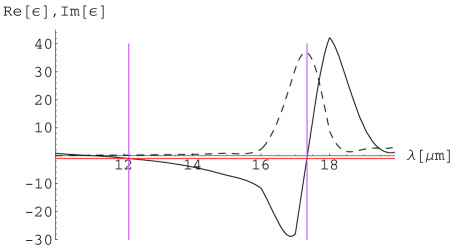
FIG. 4.: Real (solid curve) and imaginary (dashed curve) part of ${\rm Al}_{2}{\rm O}_{3}$ relative dielectric constant versus wavelength. The horizontal red line shows $-n_{m}^{2}=-1$, while the vertical magenta lines mark the two solutions $\widetilde{\lambda}_{1}$, $\widetilde{\lambda}_{2}$, of (86).

Thus, for the shell–matrix resonances, in the range $0.3\mu{\rm m}\leq\lambda\leq 20.0\mu{\rm m}$, the equation

$$\Re e\left(n_{\mbox{${\rm Al}_{2}{\rm O}_{3}$}}^{2}+n_{m}^{2}\right)=0\,,$$ (86)

has two solutions (see Fig. 4):

$$\widetilde{\lambda}_{1}\approx 12.151\mu{\rm m},$$ (87)

giving a value of

$$n_{\mbox{${\rm Al}_{2}{\rm O}_{3}$}}^{2}+n_{m}^{2}\approx 10^{-15}+0.234\,i\,,$$ (88)

and

$$\widetilde{\lambda}_{2}\approx 17.344\mu{\rm m},$$ (89)

giving a value of

$$n_{Al_{2}O_{3}}^{2}+n_{m}^{2}\approx 10^{-13}+32.611\,i\,.$$ (90)

These wavelengths are marked by magenta lines in Fig. 4. Again, the magnitude of the imaginary part of (88) and (90) shows that we may have a partial core–shell resonance at $\widetilde{\lambda}_{1}$, while the second root appears only as the result of the anomaly of $n_{\mbox{${\rm Al}_{2}{\rm O}_{3}$}}^{2}$ around $\widetilde{\lambda}_{2}$.

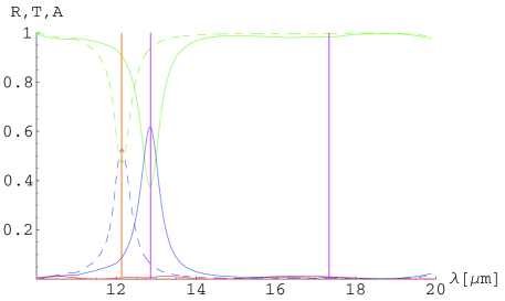
FIG. 5.: TE polarization: Reflectance (red), transmittance (green) and absorptance (blue) for a stack of solid cylinders of refractive index $n_{c}=n_{\mbox{${\rm Al}_{2}{\rm O}_{3}$}}$ and radius $r_{c}=0.03\mu$m (dashed curves), and for a stack of coated cylinders (solid curves). In both cases the stack consists of 30 gratings of cylinders, and represents a “slice” from a 2-dimensional hexagonal array. The vertical magenta lines mark the two solutions $\lambda_{1}$ and $\lambda_{2}$, of (81).

B Absorbing Core and Dielectric Shell

Here, we consider that the coated cylinders have an aluminium oxide core ($n_{c}=n_{\mbox{${\rm Al}_{2}{\rm O}_{3}$}}$), a dielectric coating ($n_{s}=n_{d}$), and are embedded in vacuum ($n_{m}=1$). The coating is a lossless, dielectric material of constant (i.e., independent of frequency) refractive index $n_{s}$=1.37. This is essentially the same as the refractive index of MgF₂ for $1\mu{\rm m}\lesssim\lambda\lesssim 2.5\mu{\rm m}$[31, 32].

1 TE Polarization

In Fig. 5 we show a comparison between two types of stacks of gratings: a stack of 30 gratings of solid cylinders having a refractive index $n_{c}=n_{\mbox{${\rm Al}_{2}{\rm O}_{3}$}}$ and radius $r_{c}=0.03\mu{\rm m}$ (dashed curves), and for a stack of 30 gratings of coated cylinders defined at the beginning of Sec. IV B (solid curves). In both cases, the period of the gratings is $d=1\mu{\rm m}$. Actually, we compare the stack of coated cylinders with a stack in which the cylinder coatings have been removed (but keeping al the other parameters unchanged), to show the influence of the shell on the optical properties of the stack (reflectance, transmittance and absorptance), for normal incidence and TE polarization.

We can see in Fig. 5 an enhancement in absorptance for the stack of coated cylinders at $\lambda_{1}$, while the stack of solid cylinders exhibits an anomalous absorptance at $\lambda_{c}\approx 12.151\mu{\rm m}<\lambda_{1}$, which corresponds to the classical resonance of a two–phase composite $n_{\mbox{${\rm Al}_{2}{\rm O}_{3}$}}^{2}+n_{m}^{2}=0$[24, 25] (in fact, the wavelength for this classical resonance, $\lambda_{c}=\widetilde{\lambda}_{1}$, is given by (86)) Thus, in the case of TE polarization there is a partial resonance of the type core–shell at $\lambda_{1}=12.861\mu{\rm m}$. At this wavelength, the anomalous increase of the absorptance of coated cylinders shows a lossy (or metallic) type behaviour, which is a characteristic of aluminium oxide and is never exhibited by the dielectric shell (lossless media). Note that the core radius is ten times smaller than the shell radius. We can also see in Fig. 6 that, at $\lambda_{1}$ the absorptance of the stack of coated cylinders (blue solid curve) is approximatively equal with the absorptance of a stack of solid cylinders, made from Al₂O₃, and having the radius $r_{s}=0.31\mu$m (blue dashed curve).

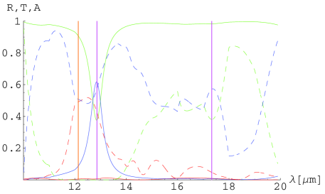
FIG. 6.: TE polarization: Reflectance (red), transmittance (green) and absorptance (blue) for a stack of solid cylinders of refractive index $n_{c}=n_{\mbox{${\rm Al}_{2}{\rm O}_{3}$}}$ and radius $r_{s}=0.31\mu$m (dashed curves), and for a stack of coated cylinders (solid curves). In both cases the stack consists of 30 parallel gratings of cylinders, and represents a “slice” from a 2-dimensional hexagonal array. The vertical magenta lines mark the two solutions $\lambda_{1}$ and $\lambda_{2}$, of (81).

Note the oscillations of the absorptance and transmittance, for the stack of solid cylinders of radius $r_{s}$ and refractive index $n_{c}$ (Fig. 6). In contrast with this behaviour, the absorptance and the transmittance of the stack of coated cylinders are almost constant, except a small region around $\lambda_{1}$. If we label by $cc$ the reflectance ($R_{cc}$), transmittance ($T_{cc}$) and absorptance ($A_{cc}$) for the stack of coated cylinders, and by $sc$ the corresponding quantities ($R_{sc}$, $T_{sc}$, $A_{sc}$) for the stack of solid cylinders, then, in the neighbourhood of the core–shell partial resonance, we have:

$$R_{cc}\approx T_{sc}\approx 0,\quad T_{cc}\approx R_{sc},\quad A_{cc}\approx A_{sc}.$$ (91)

Equation (91) shows that the equivalence between the two types of stacks is actually a sort of dualityin the sense that they have similar absorptance, but the resonant system resembles a material which absorbs and transmits the incident radiation, while the stack of ${\rm Al}_{2}{\rm O}_{3}$cylinders absorbs and reflects incident radiation.

In conclusion, at $\lambda_{1}$, for normal incidence and TE polarization, the stack of coated cylinders with a very small metallic–type core, has really the same absorptance as a stack of solid metallic cylinders of an enlarged radius $r_{s}=0.31\mu$m. It looks like the core and the shell are replaced by a new material which has the same absorptance as the core material, an effect identical with the core–shell partial resonance from electrostatics[1, 2, 3].

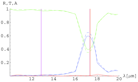
FIG. 7.: TM polarization: Reflectance (red), transmittance (green) and absorptance (blue) for a stack of solid cylinders of refractive index $n_{c}=n_{\mbox{${\rm Al}_{2}{\rm O}_{3}$}}$ and radius $r_{c}$ (dashed curves), and for a stack of coated cylinders (solid curves). In both cases the stack consists of 30 gratings of cylinders, and represents a “slice” from a 2-dimensional hexagonal array. The vertical magenta lines mark the two solutions $\lambda_{1}$ and $\lambda_{2}$, of (81).

2 TM Polarization

There is no partial resonance for a stack of coated cylinders, for TM polarization. Fig. 7 shows no change of optical characteristics around $\lambda_{1}$. The second solution of (81) is $\lambda_{2}\approx 17.333\mu{\rm m}$, and at this wavelength the stack of 30 gratings of coated cylinders exhibits an anomalous absorptance (see Fig. 7), which corresponds to the large imaginary part of (85). The stack of solid cylinders having a refractive index $n_{c}=n_{\mbox{${\rm Al}_{2}{\rm O}_{3}$}}$ and radius $r_{c}=0.03\mu{\rm m}$, exhibits an anomalous absorptance (see Fig. 7) at $\widetilde{\lambda}_{2}$, corresponding to (90).

In both cases, the anomalous high absorptance is not a resonance effect, and it is produced by an anomalous behaviour of the relative dielectric constant of ${\rm Al}_{2}{\rm O}_{3}$. At $\lambda_{2}\approx\widetilde{\lambda}_{2}$ the real part of the relative dielectric constant of ${\rm Al}_{2}{\rm O}_{3}$ is relatively small, while the imaginary part reaches a maximum value of $\approx 30$ (see Fig. 3). Therefore the absorptance of the core of coated cylinders, or of the thin cylinders of core material only becomes large (see Fig. 7). At the same time, for long wavelengths and TM polarization, the effective dielectric constant of an array of cylinders is given by the linear mixing formula (78). Thus, for an array of coated cylinders the relative effective dielectric constant is

$$\varepsilon^{*}=f_{c}\frac{\varepsilon_{c}}{\varepsilon_{m}}+f_{s}\frac{\varepsilon_{s}}{\varepsilon_{m}}+f_{m}\,,$$ (92)

while for the array of solid cylinders of core material and radius $r_{c}$ we have

$$\varepsilon^{*}=f_{c}\frac{\varepsilon_{c}}{\varepsilon_{m}}+f_{m}\,.$$ (93)

Hence, for a pure dielectric shell ($\varepsilon_{s}=$constant), in both cases, the behaviour of $\varepsilon^{*}$ is determined by $\varepsilon_{c}$ and this explains the common maximum in absorptance shown in Fig. 7, at the same position as the maximum in the imaginary part of the relative dielectric constant of ${\rm Al}_{2}{\rm O}_{3}$ (see Fig. 3). Also, around the wavelength associated with this maximum, the real part of the relative dielectric constant of ${\rm Al}_{2}{\rm O}_{3}$ exhibits a sudden jump from negative to positive values, which makes almost equal the roots of the equations (81) and (86). Actually, the anomalous absorptance exhibited by stacks of thin, solid cylinders has been described in Ref. [6].

C Dielectric Core and Absorbing Shell

Here, we consider the complementary structure with coated cylinders, having a dielectric core ($n_{c}=n_{d}$) and an aluminium oxide coating ($n_{s}=n_{\mbox{${\rm Al}_{2}{\rm O}_{3}$}}$), embedded in vacuum ($n_{m}=1$). Now, the core is a lossless, dielectric material of constant $\varepsilon_{c}$. In this case, we expect both types of partial resonances to occur, and in both cases the coated cylinder has to exhibit the characteristics of a solid cylinder made from the core material. Absorptance is a characteristic feature of the metallic phase. Therefore, we expect a decrease of the total absorptance for the stack of gratings, around $\lambda_{1}$ and $\widetilde{\lambda}_{1}$.

1 TE Polarization

For TE polarization the reflectance, transmittance and absorptance of the stack of coated cylinders with dielectric core and metallic shell, are almost the same as in the case of a stack of solid cylinders of radius $r_{s}$, made from aluminium oxide (see Fig. 8). Thus, in the neighbourhood of the shell–matrix resonance at $\widetilde{\lambda}_{1}\approx 12.151\mu{\rm m}$ the two stacks have the same optical characteristics. In fact, Eq.(66) shows that the coated cylinders must have optical characteristics similar to those of solid cylinders made from core material and of an extended radius $a=r_{s}^{2}/r_{c}$. In our case this means equivalent dielectric cylinders of radius $a=3.2\mu{\rm m}>\!\!>d/2=0.5\mu{\rm m}$, i.e. we have a stack of intersecting cylinders forming a homogeneous, dielectric slab, and we cannot apply the formulation from Sec. II. In the neighbourhood of the core–shell resonance at $\lambda_{1}\approx 12.861\mu{\rm m}$, the reflectance of the stack of coated cylinders is diminished, while the absorptance is increased, compared with a stack of aluminium oxide cylinders (Fig. 8). At $\lambda_{2}\approx\widetilde{\lambda}_{2}$ the two types of stacks exhibit identical optical characteristics, and the local maximum in absorptance appears due to the anomalous behaviour of $\varepsilon_{\mbox{${\rm Al}_{2}{\rm O}_{3}$}}$ around this wavelength (see Fig. 4).

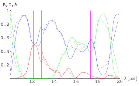
FIG. 8.: TE polarization: Reflectance (red), transmittance (green) and absorptance (blue) for a stack of solid cylinders of refractive index $n_{c}=n_{\mbox{${\rm Al}_{2}{\rm O}_{3}$}}$ and radius $r_{s}=0.31$ (dashed curves), and for a stack of coated cylinders with $r_{c}=0.03$ and $r_{s}=0.31$ (solid curves). In both cases the stack consists of 30 gratings of cylinders in a hexagonal array. The vertical magenta lines mark the solutions $\lambda_{1}$ and $\lambda_{2}$ of (81), and $\widetilde{\lambda}_{1}$ and $\widetilde{\lambda}_{2}$ of (86).

To avoid such situations when the resonant system cannot be modelled by the formulation from Sec. II, we consider a stack of coated cylinders with a larger core $r_{c}=0.21$. In this case, a shell–matrix partial resonance will lead us to an equivalent dielectric cylinder, having a radius $a=0.46\mu{\rm m}<d/2$. Now, in the neighbourhood of the shell–matrix resonance at $\widetilde{\lambda}_{1}$, the stack of coated cylinders exhibits a drop in absorptance, an increased transmittance and a very small reflectance, while a stack of aluminium oxide cylinders having the radius $r_{s}$ has a zero transmittance and equal reflectance and absorptance (see Fig. 9). The equivalent stack, formed by dielectric cylinders of radius $a$, has a zero absorptance by definition. For long wavelengths ($\lambda>d$) it has a low reflectance and a high transmittance, therefore, the only indication of the existence of a shell–matrix partial resonance is the nonzero transmittance exhibited by the coated cylinders.

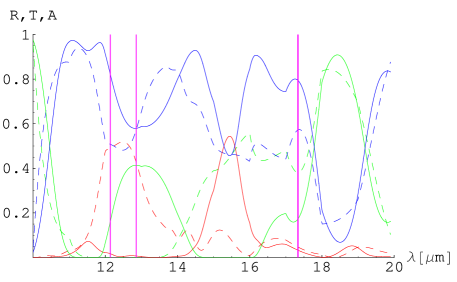
FIG. 9.: TE polarization: Reflectance (red), transmittance (green) and absorptance (blue) for a stack of solid cylinders of refractive index $n_{c}=n_{\mbox{${\rm Al}_{2}{\rm O}_{3}$}}$ and radius $r_{s}=0.31$ (dashed curves), and for a stack of coated cylinders with $r_{c}=0.21$ and $r_{s}=0.31$ (solid curves). In both cases the stack consists of 30 gratings of cylinders in a hexagonal array. The vertical magenta lines mark the solutions $\lambda_{1}$ and $\lambda_{2}$ of (81), and $\widetilde{\lambda}_{1}$ and $\widetilde{\lambda}_{2}$ of (86).

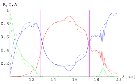
FIG. 10.: TM polarization: Reflectance (red), transmittance (green) and absorptance (blue) for a stack of solid cylinders of refractive index $n_{c}=n_{\mbox{${\rm Al}_{2}{\rm O}_{3}$}}$ and radius $r_{s}=0.31$ (dashed curves), and for a stack of coated cylinders with $r_{c}=0.03$ and $r_{s}=0.31$ (solid curves). In both cases the stack consists of 30 gratings of cylinders in a hexagonal array. The vertical magenta lines mark the solutions $\lambda_{1}$ and $\lambda_{2}$ of (81), and $\widetilde{\lambda}_{1}$ and $\widetilde{\lambda}_{2}$ of (86).

In the neighbourhood of the core–shell resonance (at $\lambda_{1}$), Fig. 9 shows a reduced absorptance for the stack of coated cylinders. Again, the equivalent stack, formed by dielectric cylinders of radius $r_{s}$, predicted by (65), has a zero absorptance by definition, and so the comparison with a stack of aluminium oxide cylinders of radius $r_{s}$, seems to be more natural. In this case, it is interesting to remark the appearance of the duality mentioned in Sec. IV B 1. The two stacks have the same absorptance and the reflectance of solid cylinders is equal with the transmittance of coated cylinders

$$R_{cc}\approx T_{sc}\approx 0,\quad T_{cc}\approx R_{sc},\quad A_{cc}\approx A_{sc}.$$ (94)

2 TM Polarization

As in the case of TE polarization, when the core radius of the coated cylinders is small (so that $a=r_{s}^{2}/r_{c}>d/2$), for TE polarization the reflectance, transmittance and absorptance of the stack of coated cylinders with dielectric core and metallic–type shell, are almost the same as in the case of a stack of solid cylinders of radius $r_{s}$, made from aluminium oxide (see Fig. 10). In fact, there is no resonant behaviour in the whole range $10\mu{\rm m}<\lambda<20\mu{\rm m}$.

In the case of a larger core of coated cylinders, the effect of shell–matrix partial resonance is small for TM polarization. Around $\lambda=\widetilde{\lambda}_{1}$ the absorptance of the coated cylinders is almost equal with their transmittance, and the reflectance is close to zero. The curves displayed in Fig. 11 show no sudden change around $\widetilde{\lambda}_{1}$ (shell–matrix partial resonance) and $\lambda_{1}$ (core–shell partial resonance), but it is interesting to remark the duality (94) at $\lambda_{1}$.

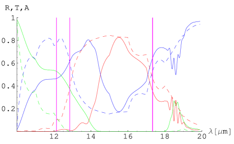
FIG. 11.: TM polarization: Reflectance (red), transmittance (green) and absorptance (blue) for a stack of solid cylinders of refractive index $n_{c}=n_{\mbox{${\rm Al}_{2}{\rm O}_{3}$}}$ and radius $r_{s}=0.31$ (dashed curves), and for a stack of coated cylinders with $r_{c}=0.21$ and $r_{s}=0.31$ (solid curves). In both cases the stack consists of 30 gratings of cylinders in a hexagonal array. The vertical magenta lines mark the solutions $\lambda_{1}$ and $\lambda_{2}$ of (81), and $\widetilde{\lambda}_{1}$ and $\widetilde{\lambda}_{2}$ of (86).

V Conclusions

We have analyzed the partial resonances of a three–phase composite, structured as a hexagonal array of coated cylinders, at long wavelengths. For such structures there are two types of partial resonances: shell–matrix and core–shell. We have shown that the shell–matrix resonance has a very small effect. In contrast, the core–shell resonance appears for TE polarization in both cases of coated cylinders metal–dielectric–vacuum and dielectric–metal– vacuum. Note that, for such resonances the stack of coated cylinders has a nonzero absorptance, so we cannot compare it with a stack of dielectric cylinders (in the case of dielectric–metal–vacuum composite). However, the comparison with a stack of solid, metallic cylinders of radius $r_{s}$ shows equal absorptance and a reflectance–transmittance duality, for the core–shell resonance.

An interesting behaviour is exhibited by the composite in the vicinity of shell–matrix ($\widetilde{\lambda}_{1}$) and core–shell ($\lambda_{1}$) resonances (see Figs. 6, 7, 9 and 11). In these regions, the composite has a very low reflectance ($R_{cc}\approx 0$), while the transmittance and absorptance take similar values.

Generally, a band gap is defined by R=1, and T=0, so that sudden changes in optical characteristics of an array of coated cylinders will change the photonic band diagram. In our calculations the partial resonances occur at long wavelengths (i.e., in the region of the acoustic band) and we expect the photonic band diagram of the composite to show horizontal lines intersecting the acoustic band. These ultrafast changes in the behaviour of a composite, due to the dependence of the refractive indexes on the wavelength, can provide the basis of future optical switches in photonic integrated circuits.

- [1] N. A. Nicorovici, R. C. McPhedran and G. W. Milton, Proc. R. Soc. Lond. A 442, 599 (1993).
- [2] N. A. Nicorovici, R. C. McPhedran and G. W. Milton, Phys. Rev. B 49, 8479 (1994).
- [3] N. A. Nicorovici, D. R. McKenzie and R. C. McPhedran, Opt. Comm. 117 151 (1955).
- [4] Lord Rayleigh, Philos. Mag. 34, 481 (1892).
- [5] L. Ohad, J. Appl. Phys. 77, 1696 (1995).
- [6] R. C. McPhedran, N. A. Nicorovici, L. C. Botten, C. M. de Sterke, P. A. Robinson and A. A. Asatryan, Opt. Comm. 168, 47 (1999).
- [7] J. B. Pendry, “Intense focusing of light using metals”, in Photonic Crystals and Light Localization in the 21st Century, ed. C. M. Soukoulis, NATO SCIENCE SERIES: C: Mathematical and Physical Sciences, Vol. 563 (Kluwer, Dordrecht, The Netherlands, 2001).
- [8] B. Gralak, S. Enoch and G. Tayeb, J. Opt. Soc. Am. A 17, 1012 (2000).
- [9] W. Y. Zhang, X. Y. Lei, Z. L. Wang, D. G. Zheng, W. Y. Tam, C. T. Chan, and Ping Sheng, Phys. Rev. Lett. 84, 2853 (2000).
- [10] R. Simon, J. R. Whinnery and T. van Duzer, Fields and waves in communication electronics (Wiley, New York, 1984).
- [11] W. K. H. Panofsky and M. Phillips, Classical electricity and magnetism, 2nd edn. (Addison-Wesley, Reading, Mass., 1962).
- [12] S. K. Chin, N. A. Nicorovici and R. C. McPhedran, Phys. Rev. E 49, 4590 (1994).
- [13] N. A. Nicorovici, R. C. McPhedran and L. C. Botten, Phys. Rev. E 52, 1135 (1995).
- [14] R. C. McPhedran, N. A. Nicorovici, L. C. Botten and K. A. Grubits, J. Math. Phys. 41, 7808 (2000).
- [15] E. G. McRae, Surface Science 11, 479 (1968); Surface Science 11, 492 (1968).
- [16] L. C. Botten, N. A. Nicorovici, A. A. Asatryan, R. C. McPhedran, C. M. de Sterke and P. A. Robinson, J. Opt. Soc. Am. A 17, 2165 (2000); J. Opt. Soc. Am. A 17, 2177 (2000).
- [17] L. C. Botten, N. A. Nicorovici, R. C. McPhedran, C. M. de Sterke, A. A. Asatryan, “Photonic band structure calculations using scattering matrices”, submitted to Phys. Rev. E.
- [18] Lord Rayleigh, Philos. Mag. 36, 365 (1918).
- [19] N. Herlofson, Arkiv. Fysik. 3, 247 (1951).
- [20] L. Tonks, Phys. Rev. 38, 1219 (1931).
- [21] D. Romell, Nature 167, 243 (1951).
- [22] J. R. Wait, Can. J. Phys. 33, 189 (1955).
- [23] J. R. Wait, Can. J. Phys. 43, 2212 (1965).
- [24] D. J. Bergman, J. Phys. C: Solid State Phys. 12, 4947 (1979).
- [25] R. C. McPhedran and D. R. McKenzie, Appl. Phys. 23, 223 (1980).
- [26] M. Abramowitz and I. A. Stegun, Handbook of mathematical functions (Dover, New York, 1972).
- [27] R. C. McPhedran, N. A. Nicorovici and L. C. Botten, J. Electromagn. Waves Appl. 11, 981 (1997).
- [28] W. T. Perrins, D. R. McKenzie and R. C. McPhedran, Proc. R. Soc. Lond. A369, 207 (1979).
- [29] C. G. Poulton, L. C. Botten, R. C. McPhedran, N. A. Nicorovici and A. B. Movchan, SIAM J. Appl. Math. 61, 1706 (2001).
- [30] O. Wiener, Abhandlungen der mathematisch–physischen Klasse der Königlich Sächsischen Gesellschaft der Wissenschaften 32, 509 (1912).
- [31] E. D. Palik, The handbook of optical constants of solids (Academic, New York, 1993).
- [32] A. Duncanson and R. W. Stevenson, Proc. Phys. Soc. Lond. 72 (1958) 1001.