Multiscale modelling of liquids with molecular specificity

Abstract

The separation between molecular and mesoscopic length and time scales poses a severe limit to molecular simulations of mesoscale phenomena. We describe a hybrid multiscale computational technique which address this problem by keeping the full molecular nature of the system where it is of interest and coarse-graining it elsewhere. This is made possible by coupling molecular dynamics with a mesoscopic description of realistic liquids based on Landau’s fluctuating hydrodynamics. We show that our scheme correctly couples hydrodynamics and that fluctuations, at both the molecular and continuum levels, are thermodynamically consistent. Hybrid simulations of sound waves in bulk water and reflected by a lipid monolayer are presented as illustrations of the scheme.

Complex multiscale phenomena are ubiquitous in nature in solid (fracture propagation Csanyi et al. (2004)), gas (Knudsen layers Garcia et al. (1999)) or in liquid phases (fluid slippage past surfaces Schmatko et al. (2005), crystal growth from fluid phase, wetting, membrane-fluid dynamics, vibrational properties of proteins in water Tarek and Tobias (2002); Baldini et al. (2005) and so on). These phenomena are driven by atomistic forces but manifest themselves at larger, mesoscopic and macroscopic scales which cannot be resolved by purely large scale molecular simulations (with some notable exceptions Vashista et al. (1997)). On the other hand, coarse-grained mesoscopic models have limited use due to the approximations necessary to treat the molecular scales intrinsic to these methods. A viable solution to this dilemma is represented by multiscale modelling via coupled models, a protocol which is also well suited to new distributed computing paradigms such as Grids Foster (2005); Coveney et al. . The idea behind this approach is simple: concurrent, coupled use of different physical descriptions.

The coupled paradigm is the underlying concept in quantum-classical mechanics hybrid schemes Csanyi et al. (2004) used to describe fracture propagation in brittle materials and also in hybrid models of gas flow Garcia et al. (1999). During the last decade, hybrid modelling of liquids has received important contributions from several research groups (see the recent review Koumoutsakos (2005)). However, it has thus far lacked the maturity to become a standard research tool for liquid and soft condensed matter systems. Hybrid simulations of liquids have been restricted to coarse-grained descriptions based on Lennard-Jones particles, reducing the major advantage of this technique of maintaining full molecular specificity where needed. Recently, new methods for energy controlled insertion of water molecules Delgado-Buscalioni and Coveney (2003b) have finally opened the way to real solvents such as water. So far, no hybrid method has employed an accurate description of the mesoscale (from nanometres to micrometres) as the important contribution of fluctuations has been neglected in the embedding coarse-grained liquid. The hybrid method must also ensure thermodynamic consistency, by allowing the open molecular system to relax to an equilibrium state consistent with the grand canonical ensemble Flekkoy et al. (2005). Finally, all previous non-equilibrium hybrid simulations have been restricted to shear flow Koumoutsakos (2005); Delgado-Buscalioni et al. (2005).

In this Letter, we present a coupled multiscale model called “hybrid MD” for simulation of mesoscopic quantities of liquids (water) embedding a nanoscopic molecular domain (Fig. 1a). Hybrid MD overcomes the limitations of previous hybrid descriptions of liquids by coupling fluctuating hydrodynamics Landau and Lifshitz (1959) and classical molecular dynamics via a protocol which guarantees mass and momentum conservation. The present method is designed to address phenomena driven by interplay between the solute-solvent molecular interaction and the hydrodynamic flow of the solvent.

Fluctuating hydrodynamics model. Our mesoscopic description of fluid flow is based on the equations of fluctuating hydrodynamics (FH) Landau and Lifshitz (1959). These equations are stochastic partial differential equations which reduce to the Navier-Stokes equations in the limit of large volumes. The equations are based on the conservation equations $\partial_{t}\phi=-\nabla\bm{J}^{\phi}$, where $\phi=\phi(\bm{r},t)$ is the density of any conserved variable at location $\bm{r}$. We consider an isothermal fluid, so that the relevant variables are the mass and momentum densities $\phi=\left\{\rho,\bm{g}\right\}$ (here $\bm{g}\equiv\rho\bm{v}$ and $\bm{v}$ is the fluid velocity). The mass and momentum fluxes are given by $\bm{J}^{\rho}=\rho\bm{v}$ and $\bm{J}^{\bm{g}}=\rho\bm{v}\bm{v}+\bm{\Pi}+\widetilde{\bm{\Pi}}$, where $\bm{\Pi}$ and $\widetilde{\bm{\Pi}}$ are the mean and fluctuating contributions to the pressure tensor, respectively. The mean pressure tensor is usually decomposed as $\mathbf{\Pi}=(p+\pi)\mathbf{1}+\mathbf{\Pi}^{S}$, where $p$ is the thermodynamic pressure (given by the equation of state) and the stress tensor is the sum of a traceless symmetric tensor $\bm{\Pi}^{S}$ and an isotropic stress $\pi$. We consider a Newtonian fluid for which $\bm{\Pi}^{S}_{\alpha\beta}=-\eta\left(\partial_{\alpha}v_{\beta}+\partial_{\beta}v_{\alpha}-2D^{-1}\partial_{\gamma}v_{\gamma}\delta_{\alpha\beta}\right)$, $\pi=-\zeta\partial_{\gamma}v_{\gamma}$, where repeated indices are summed, $D$ the spatial dimension and $\eta$, $\zeta$ are the shear and bulk viscosities respectively. The components of the fluctuating pressure tensor $\widetilde{\Pi}_{\alpha\beta}$ are random Gaussian numbers (see supplementary information).

Our continuum mesoscopic model is based on a finite volume discretization of the FH equations Serrano and Español (2001), although here in an Eulerian frame of reference and on a regular lattice. Partitioning the space into several space-filling volumes $V_{k}$ with $k=1,...,N$ centered at positions $\bm{r}_{k}$, we integrate the conservation equations over each volume $V_{k}$ and apply Gauss’ theorem $\frac{d}{dt}\int_{V_{k}}\phi(\mathbf{r}_{k},t)d\mathbf{r}=\sum\limits_{l}A_{kl}\mathbf{J}^{\phi}_{kl}\cdot\mathbf{e}_{kl}$, where $\mathbf{e}_{kl}$ is the unit surface vector pointing towards cell $k$, and $A_{kl}$ is the surface area connecting cells $k$ and $l$. We then derive the following stochastic equations for mass and momentum exchange:

$$dM_{k}^{t} =\sum_{l}\mathbf{g}_{kl}\cdot\mathbf{e}_{kl}A_{kl}dt,$$ (1)

$$d\mathbf{P}_{k}^{t} =\sum_{l}\left[\frac{\bm{\Pi}_{l}}{2}\cdot\mathbf{e}_{kl}+\mathbf{g}_{kl}\cdot\mathbf{e}_{kl}\mathbf{v}_{kl}\right]A_{kl}dt+d\widetilde{\mathbf{P}}_{k}^{t},$$ (2)

where $d\widetilde{\mathbf{P}_{k}}$ is the momentum exchange due to the fluctuating pressure tensor $\widetilde{\Pi}_{k}$, ${\bf v}_{kl}={\bf v}_{k}-{\bf v}_{l}$ and $\mathbf{g}_{kl}$ is approximated on the surface kl by $\mathbf{g}_{kl}=\frac{1}{2}(\rho_{k}+\rho_{l})\frac{1}{2}(\mathbf{v}_{k}+\mathbf{v}_{l})$. To close the discrete conservation equations we have to devise a discretization of the dissipative and fluctuating parts which ensures the validity of the fluctuation-dissipation theorem. By choosing the discretization of the gradients $\partial^{\alpha}\phi_{k}\rightarrow\sum_{l}A_{kl}\bm{e}^{\alpha}_{kl}\phi_{k}/(2V_{k})$, the discrete momentum fluxes $\mathbf{\Pi}_{k}$ and $d\widetilde{\mathbf{P}}_{k}$ take the form given in Serrano and Español (2001) (see also supplementary information). The resulting set of stochastic differential equations Eqs. (1,2) may be integrated using various stochastic integration schemes De Fabritiis et al. (2006); in this work we have used a simple Euler scheme.

Molecular dynamics. The molecular description is based on classical molecular dynamics and the CHARMM27 forcefield (incorporating the TIP3P parametrization) which specifies bond, angle, dihedral and improper bonded interactions and non-bonded Lennard-Jones 6-12 and Coulomb interactions. The code is derived from a stripped down version of NAMD Kalé et al. (1999). We use a dissipative particle dynamics (DPD) thermostat Soddemann et al. (2003) ensuring local momentum conservation in such a way that hydrodynamic modes are not destroyed.

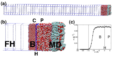
Figure 1: The set-up used for our hybrid molecular simulations (a) and a close-up of the hybrid interface (b). The fluctuating hydrodynamics description (FH), resolved by the finite volume method, is coupled to a molecular model (MD) representing a dimyristoylphosphatidylcholine (DMPC) lipid monolayer solvated with water and restrained at the lipid head groups. We indicate by “P” and “C” respectively the particle and continuum cells adjacent to the hybrid interface “H”. The buffer region of the MD system “B” (overlapping the C cell) is indicated by translucent water molecules and the water molecule density in the buffer region is shown in (c).

Coupling protocol.- In our computational implementation, the MD and FH components are independent coupled models Coveney et al. which exchange information after every fixed time interval $\Delta t_{c}$. We set $\Delta t_{c}=n_{FH}\Delta t=n_{MD}\delta t$, where $\Delta t$ and $\delta t$ are the FH and MD time steps and, $n_{FH}$ and $n_{MD}$ are integers which depend on the system being modeled; e.g. for water as solvent $\Delta t_{c}=100$ fs, $n_{FH}=10$ and $n_{MD}=100$. Conservation is based on the flux balance: both domains receive equal but opposite mass and momentum fluxes across the hybrid interface. This interface (H) uniquely defines the total system (MD+FH, see Fig. 1b) and, importantly, the total quantities to be conserved. This contrasts with previous schemes Koumoutsakos (2005) where particle and continuum domains intertwine within a larger overlapping region, preventing a clear definition of the system.

The rate of momentum transferred across the hybrid interface is given by ${\bf F}_{H}=A\bm{J}^{\bm{g}}_{H}\cdot\bm{e}_{\perp}$, where $\bm{e}_{\perp}$ is the unit vector perpendicular to the surface and the momentum flux tensor at “H” is approximated as $\bm{J}^{\bm{g}}_{H}=(\bm{J}^{\bm{g}}_{P}+\bm{J}^{\bm{g}}_{C})/2$. Note that $\bm{J}^{\bm{g}}_{C}$ involves the evaluation of the discretized velocity gradient at $C$, and thus requires the mass and momentum of the MD system at the neighbouring P cell averaged over the coupling time $\Delta t_{C}$: $\langle M_{P}\rangle_{\Delta t_{c}}$ and $\langle\bm{P}_{P}\rangle_{\Delta t_{c}}$, respectively (see Fig. 1b). On the other hand, the momentum flux tensor at the P cell can be computed for the microstate using the kinetic theory formula $\bm{J}^{\bm{g}}_{P}=\langle[\rho{\bf v}_{i}{\bf v}_{i}+W_{i}]\rangle_{\Delta t_{c}}$, with $i\in P$ and $W_{i}=\sum_{j}{\bf r}_{ij}\cdot{\bf f}_{ij}$ M. P. Allen and D. J. Tildesley (1987) being the contribution of atom $i$ to the virial. Alternatively, $\bm{J}^{\bm{g}}_{P}$ can be computed by introducing the coarse-grained variables at the neighboring MD and FH cells into the discretized Newtonian constitutive relation. Both approaches provide equivalent results in terms of mean and variance of the pressure tensor.

The force ${\bf F}_{H}$ at the hybrid interface is imposed on the FH domain using standard von Neumann boundary conditions. In order to impose the force $-{\bf F}_{H}$ on the molecular system, we extend the MD domain to an extra buffer cell (“B” in Fig. 1b). Particles are free to cross the hybrid interface according to their local dynamics, but any atom that enters in B will experience an external force $-{\bf F}_{H}/N_{B}$ which transfers the external pressure and stress. The number of solvent molecules at the buffer $N_{B}(t)$ is controlled by a simple relaxation algorithm: $\Delta{N}_{B}=(\langle N_{B}\rangle-N_{B})\Delta t_{c}/\tau_{B}$, with $\tau_{B}\simeq 500$ fs. The average $\langle N_{B}\rangle$ is set so as to ensure that B always contains enough molecules to support the momentum transfer; here we use $\langle N_{B}\rangle=0.75M_{C}/m$, where $M_{C}$ is the mass of the continuum cell C and $m$ the molecular mass. Figure 1c shows the equilibrium number density profile of water at the buffer. Importantly, the density profile is flat around the hybrid interface. Due to the external pressure, it quickly vanishes near the open boundary. In fact, molecules eventually reaching this rarefied region in B are removed. If the relaxation equation requires $\Delta N_{B}>0$, new molecules are placed in B with velocities drawn from a Maxwellian distribution with mean equal to the velocity at the C cell. The insertion location is determined by the usher algorithm Delgado-Buscalioni and Coveney (2003b), which efficiently finds new molecule configurations releasing an energy equal to the mean energy per molecule. Momentum exchange due to molecule insertion/removal is taken into account in the overall momentum balance Flekkoy et al. (2005).

In fluid dynamics the mass flux is not an independent quantity but is controlled by the momentum flux [see Eqs. (1) and (2)]. Consequently, we do not explicitly impose the mass flux on the MD system. Instead it arises naturally from the effect of the external pressure on the molecule dynamics near the interface. The mass flux $\bm{J}^{\rho}_{H}\cdot\bm{e}_{\perp}$ is thus measured (via simple molecule count) from the amount of MD mass crossing the interface H over the coupling time $\Delta t_{c}$. The opposite of this flux is then transfered to the adjacent C cell via a simple relaxation algorithm Flekkoy et al. (2005), using a relaxation time ($\tau_{r}\geq O(100)$ fs) large enough to preserve the correct mass distribution at the C cell, but still much faster than any hydrodynamic time. This guarantees mass conservation.

Results. We first test the conservation of the total mass $M$ and momentum ${\bm{P}}$. Results are shown in Fig. 2a, where we consider the equilibrium state of a hybrid MD simulation of water in a 3D periodic box $50\times 50\times 735$ $\mathrm{\AA}^{3}$ (each cell is $50\times 50\times 15$ $\mathrm{\AA}^{3}$). The embedded TIP3P water domain (including the buffers) is $75\mathrm{\AA}$ wide in the coupling (z) direction and was pre-equilibrated at 1 atm and 300K. Figure 2a shows the mean error in mass and momentum conservation. As stated above, mass conservation is ensured over a short time $\Delta t_{c}\sim O(100)$ fs, as clearly reflected in Fig. 2a. However, as the external force is imposed within the buffers B, the momentum conservation is ensured only on the “extended” system (MD+FH+B). The variation of momentum of the total system (MD+FH) is then a small bounded quantity whose time average becomes smaller than the thermal noise after about 1ps (see Fig. 2a), i.e, faster than any hydrodynamic time scale.

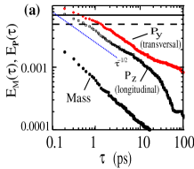
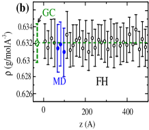
Figure 2: (a) The normalized mean error in mass $E_{M}(\tau)$ and momentum $E_{P_{\alpha}}(\tau)$ evaluated as $E_{A}^{2}(\tau)=\langle[\int_{t_{0}}^{t_{0}+\tau}\delta A(t)dt/\tau]^{2}\rangle_{t_{0}}/\langle M_{k}\rangle^{2}$, with $\delta A=A-\langle A\rangle$. The dashed and solid horizontal lines are, respectively, the normalized standard deviation of mass and momentum within one cell ($\sigma[M_{k}]/\langle M_{k}\rangle$). (b) Density field in a hybrid MD equilibrium simulation of water. Solid circles corresponds to MD cells. Error bars are the standard deviation of each cell density. The grand-canonical (GC) result is $\langle\rho\rangle=0.632\mathrm{g/mol/\AA^{3}}$ and $\sigma[\rho]=0.0045\mathrm{g/mol/\AA^{3}}$.

The FH description uses an accurate interpolated equation of state $p(\rho)=(3.84-15.7\rho+15.3\rho^{2})\,10^{4}$ bars, which fits for $\rho=[0.54,0.70]$ $\mathrm{g/mol/A^{3}}$ the outcome of $NPT$ simulations of TIP3P water at $T=300$K and provides quasi-perfect match of the mean pressure, density (see Fig. 2b) and sound velocity. The shear and bulk viscosities of the FH model are assigned to match those of the MD fluid (for water at $T=300$K we used those reported in Ref. Guo and Zhang (2001)). Also, in cases where the viscosity varies locally, the FH model allows one to assign a different viscosity for each cell. Momentum fluctuations at each cell are consistently controlled by the DPD thermostat in the MD region, and via the fluctuation-dissipation balance in the FH domain. Density fluctuations present a much more stringent test of thermodynamic consistency. Each fluid cell is an open subsystem so, at equilibrium, its mass fluctuation should be governed by the grand canonical (GC) prescription: $\sigma[\rho]=[\rho k_{B}T/(V_{k}c_{T}^{2})]^{1/2}$ Landau and Lifshitz (1959) (where $\sigma$ means standard deviation and $c_{T}^{2}\equiv(\partial P/\partial\rho)_{T}$ is the squared sound velocity at constant temperature). Mass fluctuations within the MD and FH cells are both in agreement with the GC result (Fig. 2b) indicating that neither the usher molecule insertions Delgado-Buscalioni and Coveney (2003b) nor the mass relaxation algorithm substantially alter the local equilibrium around the interface H.

We now focus on transmission of sound waves which thus far have remained an open problem in the hybrid setting. In a slot of water between rigid walls we perturb the equilibrium state with a Gaussian density perturbation (amplitude 5% and standard deviation $45\mathrm{\AA}$). As shown in Fig. 3a the resulting travelling waves cross the MD domain several times at the center of the slot. Sound waves require fast mass and momentum transfer as any significant imbalance would generate unphysical reflection at the hybrid interface. No trace of reflection is observed and comparison with full FH simulations shows statistically indistinguishable results.

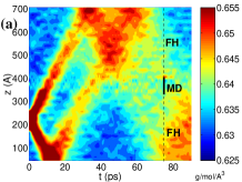
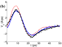
Figure 3: (a) Spatio-temporal diagram along $z$ for the density field of a three-dimensional simulation of two sound waves traveling within a closed box filled with water. The region of width $45\mathrm{{\AA}}$ around the centre of the box is described with molecular dynamics (MD), while the rest of the domain is solved via fluctuating hydrodynamics (FH). (b) The longitudinal velocity arising from the interaction between a sound wave and a grafted lipid layer (set up of Fig. 1a). We compare hybrid MD (solid line), full MD (circles) and full FH simulation using purely reflecting walls (dashed line). Results are averaged over $15$ nm from the monolayer; error bars indicate the standard deviation over 10 runs.

Finally, we validate the hybrid scheme against full MD simulations of complex fluid flow (set-up Fig. 1a). A sound wave generated by a similar Gaussian perturbation is now reflected against a lipid monolayer (DMPC) (Fig. 3b). Each lipid is tethered by the heavy atoms of the polar head group with an equilibrated grafting cross-section of 53 $\mathrm{{\AA}}^{2}$/lipid, close to the experimental cross-section of membranes. In the hybrid simulation, the MD water layer close to the lipid membrane extends just $45\mathrm{\AA}$ above it (see Fig. 1b). Instead, in the MD simulation we considered a large $180\times 50\times 50$ $\mathrm{\AA}^{3}$ box of explicit water containing around 50K atoms. The wave velocity near the layer is compared in Fig. 3b for the hybrid MD and MD simulations. The excellent agreement demonstrates that the coupling protocol accurately resolves features produced by the molecular structure. In Fig. 3b such effects are due to sound absorption by the lipid layer, highlighted by comparison with a FH simulation of the same wave impinging against a purely reflecting wall. The present sound waves simulations were done assuming an isothermal environment. This is realistic if the rate of thermal relaxation $D_{T}k^{2}$ (with $D_{T}\sim 1.5\times 10^{-7}m/s^{2}$ the water thermal diffusivity and $k=2\pi/\lambda$ the wavenumber) is comparable with or faster than its sound frequency $c\,k$. The present simulations $\lambda\sim 50\AA$ are just in the limit of the isothermal sound regime Cowan et al. (1996), while waves with $\lambda>O(10)\AA$ propagate adiabatically and require consideration of the energy flow Flekkoy et al. (2005).

In summary, we have presented a stable and robust multiscale method (hybrid MD) for the simulation of the liquid phase which embeds a small region, fully described by chemically accurate molecular dynamics, into a fluctuating hydrodynamics representation of the surrounding liquid. Mean values and fluctuations across the interface are consistent with hydrodynamics and thermodynamics. Sound waves propagating through the MD domain and flow behavior arising from the interaction with complex molecules are both treated correctly. We considered water waves reflected by DMPC monolayers, but the scope of this methodology is much broader, including inter alia the study of vibrational properties of hydrated proteins (via high frequency perturbations) Tarek and Tobias (2002); Baldini et al. (2005), the ultrasound absorption of complex liquids Almagor et al. (1990) or the simulation of quartz crystal oscillators Broughton et al. (1997) for the study of complex fluid rheology or slip flow past surfaces Schmatko et al. (2005).

GDF&PVC acknowledge projects Integrative Biology (GR/S72023) and IntBioSim (BBS/B/16011). RD-B acknowledges projects MERG-CT-2004-006316, CTQ2004-05706/BQU and FIS2004-01934. We thank M. Serrano, A. Dejoan, S. Succi, P. Español and E. Flekkøy.

References

- Csanyi et al. (2004) G. Csanyi, T. Albaret, M. C. Payne, and A. D. Vita, Phys. Rev. Lett. 93, 175503 (2004)
- Garcia et al. (1999) A. Garcia, J. Bell, W. Y. Crutchfield, and B. Alder, J. Comp. Phys. 154, 134 (1999).
- Schmatko et al. (2005) T. Schmatko, H. Hervet, and L. Leger, Phys. Rev. Lett. 94, 244501 (2005). C. Neto, D. R. Evans, E. Bonaccurso, H.-J. Butt, and V. S. J. Craig, Rep. Prog. Phys. (2005).
- Tarek and Tobias (2002) M. Tarek and D. J. Tobias, Phys. Rev. Lett. 89, 275501 (2002).
- Baldini et al. (2005) G. Baldini, F. Cannone, and G. Chirico, Science 309, 1096 (2005).
- Vashista et al. (1997) P. Vashista, R. K. Kalia, W. Li, A. Nakano, A. Omeltchenko, K. Tsuruta, J. Wang, and I. Ebbsjö, Curr. Opinion Solid Stat. Mat. Sci. 1, 853 (1996).
- Foster (2005) I. Foster, Science 6, 814 (2005).
- (8) P. V. Coveney, G. De Fabritiis, M. Harvey, S. Pickles, and A. Porter, in press Comp. Phys. Comm. (2006) [http://arxiv.org/abs/physics/0605171].
- Koumoutsakos (2005) P. Koumoutsakos, Ann. Rev. Fluid Mech. 37, 457 (2005).
- Delgado-Buscalioni and Coveney (2003b) G. De Fabritiis, R. Delgado-Buscalioni, and P. V. Coveney, J. Chem. Phys. 121, 12139 (2004). R. Delgado-Buscalioni and P. V. Coveney, J. Chem Phys. 119, 978 (2003b).
- Flekkoy et al. (2005) E. G. Flekkoy, R. Delgado-Buscalioni, and P. V. Coveney, Phys. Rev. E 72, 026703 (2005). R. Delgado-Buscalioni and P. V. Coveney, Phys. Rev. E 67, 046704 (2003a).
- Delgado-Buscalioni et al. (2005) R. Delgado-Buscalioni, E. Flekkøy, and P. V. Coveney, Europhys. Lett. 69, 959 (2005).
- Landau and Lifshitz (1959) L. D. Landau and E. M. Lifshitz, Fluid mechanics (Pergamon Press, New York, 1959).
- Serrano and Español (2001) M. Serrano and P. Español, Phys. Rev. E 64, 046115 (2001). E. G. Flekkøy, P. V. Coveney, and G. De Fabritiis, Phys. Rev. E 62, 2140 (2000).
- De Fabritiis et al. (2006) G. De Fabritiis, M. Serrano, P. Español, and P. V. Coveney, Physica A 361, 429 (2006).
- Kalé et al. (1999) L. Kalé, R. Skeel, M. Bhandarkar, R. Brunner, A. Gursoy, N. Krawetz, J. Phillips, A. Shinozaki, K. Varadarajan, and K. Schulten, J. Comp. Phys. 151, 283 (1999).
- Soddemann et al. (2003) T. Soddemann, B. Dunweg, and K. Kremer, Phys. Rev. E 68, 046702 (2003).
- M. P. Allen and D. J. Tildesley (1987) M. P. Allen and D. J. Tildesley, Computer Simulations of Liquids (Oxford University Press, Oxford, 1987).
- Guo and Zhang (2001) G. Guo and Y. Zhang, Mol. Phys. 99, 283 (2001).
- Almagor et al. (1990) A. Almagor, S. Yedgar, and B. Gavish, Biorheology 27, 605 (1990).
- Cowan et al. (1996) M. Cowan, J.. Rudnick, and M. Barnatz Phys. Rev. E 53, 4490 (1996).
- Broughton et al. (1997) J. Q. Broughton, C. A. Meli, P. Vashista and R. K. Kalia, Phys. Rev. B 56, 611 (1997).