Kinetic Vlasov Simulations of collisionless magnetic Reconnection

Abstract

A fully kinetic Vlasov simulation of the Geospace Environment Modeling (GEM) Magnetic Reconnection Challenge is presented. Good agreement is found with previous kinetic simulations using particle in cell (PIC) codes, confirming both the PIC and the Vlasov code. In the latter the complete distribution functions $f_{k}$ ($k=i,e$) are discretised on a numerical grid in phase space. In contrast to PIC simulations, the Vlasov code does not suffer from numerical noise and allows a more detailed investigation of the distribution functions. The role of the different contributions of Ohm’s law are compared by calculating each of the terms from the moments of the $f_{k}$. The important role of the off–diagonal elements of the electron pressure tensor could be confirmed. The inductive electric field at the X–Line is found to be dominated by the non–gyrotropic electron pressure, while the bulk electron inertia is of minor importance. Detailed analysis of the electron distribution function within the diffusion region reveals the kinetic origin of the non–gyrotropic terms.

I Introduction

Magnetic reconnection is the fundamental process which allows magnetized plasmas to convert the energy stored in the field lines into kinetic energy of the plasma. It plays an important role in the dynamics of space and laboratory plasmas. In the magnetopause it allows particles from the solar wind to enter the magnetosphere. Also it is believed to be the main source of energy for solar flares and coronal mass ejections.

In ideal magnetohydrodynamics (MHD) the frozen–in flux condition prohibits the magnetic field topology to change. Thus reconnection depends on a mechanism that breaks the frozen–in condition. This non–ideal mechanism is responsible for the dynamics of the diffusion region, where the topology change takes place. In resistive MHD with low values of resistivity an elongated Sweet–Parker current sheet develops, which limits the reconnection rate. Parker:57 ; Sweet:58 ; Biskamp:86 Higher values for the resistivity, on the other hand, are extremely unrealistic for the astrophysical reconnection processes.

In the last years it has become apparent that the minimal model to adequately describe collisionless reconnection is Hall–MHD. Shay:01 ; Lottermoser-Scholer:1997 ; Wang-etal:2001 ; Huba-Rudakov:2004 In Hall–MHD the ion inertial length $\lambda_{i}$ is introduced as a characteristic scale length such that for distances smaller than $\lambda_{i}$ the ion dynamics can decouple from the magnetic field. Within the framework of the Geospace Environmental Modeling (GEM) Magnetic Reconnection Challenge a two dimensional magnetic reconnection setup based on the Harris equilibrium was studied. Simulations were done using MHD models with constant or localized resistivity Birn:2001b ; Otto:2001 , Hall–MHD models Birn:2001b ; Otto:2001 ; Ma:2001 , hybrid models where electrons are treated as fluid and ions are treated kinetically Shay:01 ; Kuznetsova:2001 and with fully kinetic particle codes. Shay:01 ; Pritchett:2001b ; Hesse:2001 The models which included the Hall effect, either directly or implicitly in the kinetic treatment, showed very similar results in terms of the global reconnection rate. The small scale structures of the dissipation region, on the other hand, varied substantially between the models. In Ref. Birn:2001a, it was concluded that the large scale ion dynamics control the rate of reconnection and that the dispersive character of Whistler modes is essential in the understanding of the results.

These results emphasize the importance of the Hall term for the reconnection. At the neutral X–line, the magnetic field strength is exactly zero and the Hall term vanishes. Only the electron bulk inertia and the non–gyrotropic part of the electron pressure tensor can yield a contribution at the X–line. Kuznetsova et al. Kuznetsova:1998 pointed out, that the bulk inertia of the electrons can only contribute if the current sheet develops on electron timescales. Vasyliunas Vasyliunas:1975 was the first to emphasize the important role of the off–diagonal components of the pressure tensor in the diffusion region. Later their role was investigated by a number of authors (see e.g Refs. Dungey:1988, ; Hesse:1993, ; Kuznetsova:1998, ; Kuznetsova:2001, ). The non–gyrotropic pressure can be understood as originating from the meandering motion of the electrons, which bounce in the magnetic field reversal region, also known as Speiser motion. Speiser:1991

In this study, we use a Vlasov code to investigate the GEM reconnection. In contrast to Particle–In–Cell (PIC) codes, Vlasov codes discretise the complete distribution functions of electrons and ions on a grid in phase space. This has the advantage of allowing more detailed investigations of the distribution functions, since numerical noise is completely absent from the Vlasov–approach. The main focus of our investigation is the electron dynamics. These can be understood in two ways. On one hand, one can take a microscopic point of view by looking at the detailed structure of the distribution function. On the other hand one can look at the moments of the distribution function and their importance for Ohm’s law. The Vlasov–approach allows us to do both with very high accuracy.

In the next section we briefly present the methods used in our investigation. The GEM reconnection setup including the initial conditions and the boundary conditions is described in section III. In section IV we discuss the results. Separate subsections are dedicated to the discussion of the contributions of the terms in Ohm’s law, especially the off–diagonal components of the pressure tensor, and to the detailed discussion of the electron distribution function. Section V will give a summary and present conclusions.

II Methods

The basis of the kinetic description of magnetic reconnection are the distribution functions $f_{k}({\bf x},{\bf v},t)$ of species $k$, where $k=i,e$ denotes ions or electrons. The temporal behavior of the distribution function is given by the Vlasov equation

$$\frac{\partial f_{k}}{\partial t}+{\bf v}\cdot\nabla f_{k}+\frac{q_{k}}{m_{k}}\left({\bf E}+{\bf v}\times{\bf B}\right)\cdot\nabla_{\bf v}f_{k}=0.$$

Here $q_{k}$ and $m_{k}$ are the charge and the mass of the particles of species $k$. The Vlasov equation describes the incompressible flow of the species phase space densities under the influence of the electromagnetic fields.

The fields are solved using the Darwin approximation (see, for example Refs. BIR85, ; SCHM06a, )

$$\nabla\times\mathbf{E}_{T} =-\frac{\partial\mathbf{B}}{\partial t}\;\;,$$ (1)

$$\frac{1}{\mu_{0}}\nabla\times\mathbf{B} =\varepsilon_{0}\frac{\partial\mathbf{E}_{L}}{\partial t}+{\bf j}\;\;,$$ (2)

$$\nabla\cdot\mathbf{E}_{L} =\frac{1}{\varepsilon_{0}}\rho\;\;,$$ (3)

$$\nabla\cdot\mathbf{B} =0\;\;,$$ (4)

where $\mathbf{B}$ is the magnetic and $\mathbf{E}_{L}$ and $\mathbf{E}_{T}$ are the longitudinal and the transverse part of the electric field, $\nabla\times\mathbf{E}_{L}=0$, $\nabla\cdot\mathbf{E}_{T}=0$, $\mathbf{E}=\mathbf{E}_{L}+\mathbf{E}_{T}$. The Darwin approximation eliminates the fast electromagnetic vacuum modes while all other plasma modes are still described. Instead of neglecting the displacement current completely, only its transverse part is dropped while its longitudinal part is kept. The elimination of the vacuum modes allows larger time-steps in the simulation since only the slower non–relativistic waves have to be resolved.

The charge density $\rho$ and the current density $\mathbf{j}$ are given by the moments of the distribution function,

$$\rho =\sum_{k}q_{k}\int f_{k}(\mathbf{x},\mathbf{v})d^{3}v\;\;,$$ (5)

$$\mathbf{j} =\sum_{k}q_{k}\int\mathbf{v}f_{k}(\mathbf{x},\mathbf{v})d^{3}v\;\;.$$ (6)

These moments couple the electromagnetic fields back to the distribution function. In this way the Vlasov-Darwin system constitutes a non–linear system of partial integro–differential equations.

For the simulations we use a $2\frac{1}{2}$–dimensional Vlasov–code described in Ref. SCHM06a, . Here $2\frac{1}{2}$–dimensional means, we restrict the simulations to 2 dimensions in space but include all three velocity dimensions. In contrast to PIC–codes, the distribution function is integrated in time directly on a numerical grid in phase space. The integration scheme is based on a flux conservative and positive scheme FIL01 which obeys the maximum principle and suffers from relatively little numerical diffusion. The main idea of the scheme is to calculate the fluxes into and out of a grid cell by interpolating the primitive of the distribution function. The one dimensional scheme has been generalized to two spatial and three velocity dimensions using the backsubstitution method described in Ref. SCHM06b, . The backsubstitution method has been shown to be slightly superior and, more importantly, much faster than the straightforward time–splitting scheme.

The Maxwell equations in the Darwin approximation can be recast into a form which does not include any time derivatives (see, for example, Refs. BIR85, ; SCHM06a, ). This makes it possible to express the electromagnetic fields $\mathbf{E}(t_{0})$, $\mathbf{B}(t_{0})$ at any time $t_{0}$ by the density $\rho(t_{0})$ and the current density $\mathbf{j}(t_{0})$ at the time $t_{0}$. No time integration of the fields is necessary and the conditions $\nabla\cdot\mathbf{B}=0$ and $\nabla\cdot\mathbf{E}=\rho$ are always met by construction.

III GEM Reconnection Setup

The reconnection setup is identical to the parameters of the GEM magnetic reconnection challenge. Birn:2001a The initial conditions are based on the Harris sheet equilibrium HARS62 in the $x$,$y$–plane

$$\mathbf{B}(y)=B_{0}\tanh\left(\frac{y}{\lambda}\right)\mathbf{\hat{x}}.$$ (7)

The particles have a shifted Maxwellian distribution

$$f_{0i,e}(y,\mathbf{v})=n_{0}(y)\exp\left[\frac{m_{i,e}}{2T_{i,e}}\left(v_{x}^{2}+(v_{y}-V_{0i,e})^{2}+v_{z}^{2}\right)\right].$$ (8)

Here $T_{i,e}$ are the constant electron and ion temperatures and $V_{0i,e}$ are the constant electron and ion drift velocities. The density distribution is then given by

$$n_{0}(y)=n_{0}\text{ sech}^{2}\left(\frac{y}{\lambda}\right).$$ (9)

The Harris equilibrium demands that

$$\frac{B_{0}^{2}}{2\mu_{0}} =n_{0}(T_{i}+T_{e})$$ (10)

$$\lambda =\frac{2}{eB_{0}}\frac{T_{i}+T_{e}}{V_{0i}-V_{0e}}$$ (11)

$$\text{and}\qquad\frac{V_{0e}}{V_{0i}} =-\frac{T_{e}}{T_{i}}.$$ (12)

In addition a uniform background density $n_{b}=0.2n_{0}$ with the same temperature $T_{i,e}$ but without a directed velocity component is included.

The total GEM system size is $L_{x}=25.6\lambda_{i}$ in $x$–direction and $L_{y}=12.8\lambda_{i}$ in $y$–direction, where $\lambda_{i}$ is the ion inertial length $\lambda_{i}=c/\omega_{pi}$ with the ion plasma frequency is defined using the given by $\omega_{pi}=(ne^{2}/\varepsilon_{0}m_{i})^{1/2}$. Because of the symmetry constraints we simulate only one quarter of the total system size: $0\leq x\leq L_{x}/2$ and $0\leq y\leq L_{y}/2$. The sheet half thickness is chosen to be $\lambda=0.5\lambda_{i}$. The temperature ratio is $T_{e}/T_{i}=0.2$ and a reduced mass ratio of $m_{i}/m_{e}=25$ is used. This reduced mass ratio is consistent with the GEM setup and was chosen as a compromise between a good separation of scales (both in space and time) and the computational effort. The numerical expense was especially high for the kinetic codes. Shay:01 ; Pritchett:2001b ; Hesse:2001 The reduced mass ratio was also used in the hybrid codes Shay:01 ; Kuznetsova:2001 for the sake of comparison. A higher mass ratio (i.e. a smaller electron mass) results in a smaller electron skin depth which has to be resolved by the grid. At the same time the numerical time step has to be reduced to resolve the electron Larmor frequency. Both effects together imply that, in a spatially two–dimensional simulation, the computational cost increases with the square of the mass ratio for all kinetic simulations independent whether thay use PIC or Vlasov–methods. Simulations with substantially higher mass ratios using the generally more demanding Vlasov approach, therefore, currently seem out of reach. The simulation is performed on $256\times 128$ grid points in space for the quarter simulation box. This corresponds to a resolution of $512\times 256$. This implies a grid spacing of $\Delta x=\Delta y=0.05\lambda_{i}$. The resolution in the velocity space was chosen to be $20\times 20\times 40$ grid points. In $v_{z}$ direction the grid was extended to account for the electron acceleration in the diffusion region. The simulation was performed on a 32 processor Opteron cluster and took approximately 150 hours to complete.

An initial perturbation

$$\psi(x,y)=\psi_{0}\cos(2\pi x/L_{x})\cos(\pi y/L_{y})$$ (13)

is added to the magnetic vector potential component $A_{z}$. The magnitude of the perturbation is chosen to be $\psi_{0}=0.1B_{0}/\lambda_{i}$. The rather high values of the initial perturbation generates a single large magnetic island. The initial linear growth of the tearing mode is bypassed and the system is placed directly in the nonlinear regime. The reason for this relatively strong perturbation is that the initial growth of the instabilities depends strongly on the electron model. In contrast to this, the GEM challenge demonstrated convincingly, that the later nonlinear stage is not sensitive to the details of the underlying model.

IV Simulation Results

Figure 1: Time evolution of the reconnected magnetic flux $\Psi$ throughout the simulation run.

As a measure of the reconnected magnetic field we use the difference $\Delta\Psi$ of the magnetic vector potential component $A_{z}$ between the X–point and the O–point. Figure 1 shows the reconnected magnetic flux as a function of time. The evolution of $\Delta\Psi$ agrees very well with the results of other simulations of the GEM challenge. Birn:2001a After an initial small increase, the flux starts to rapidly increase at $t\Omega_{i}\approx 15$. A value of $\Delta\Psi=B_{0}/\lambda_{i}$ is reached at $t\Omega_{i}\approx 17.7$. This is slightly later to what is observed in the PIC simulations. Pritchett Pritchett:2001b reports a time $t\Omega_{i}\approx 15.7$ where the same flux level is reached. While the level of saturation is comparable to the other GEM results, it is again reached slightly later than in Ref. Pritchett:2001b, at time $t\Omega_{i}\approx 30$.

The upper panel of Figure 2 shows the out of plane magnetic field $B_{z}$ at $\Omega_{i}t=17.7$. One can clearly identify the quadrupolar structure generated by the Hall currents. SONN79 ; TER83 The peak value of the magnetic field $|\mathbf{B_{z}}|$ in the island structure is $\approx 0.17B_{0}$ and is located at $|x|\approx 1.7\lambda_{i}$. This is a somewhat lower magnetic field than in Ref. Pritchett:2001b, and is also located slightly closer to the X–line. In the course of the simulation both the size of the magnetic island and the magnitude of the peak magnetic field increase. For this reason, the differences to the PIC simulations can be attributed to the small differences in the temporal behavior. This also explains the magnetic field towards the top and bottom boundaries of the simulation box. These fields, which can be seen in Figure 2, have essentially disappeared at $\Omega_{i}t=20$, approximately the same time that the peak magnetic reconnection rate is seen.

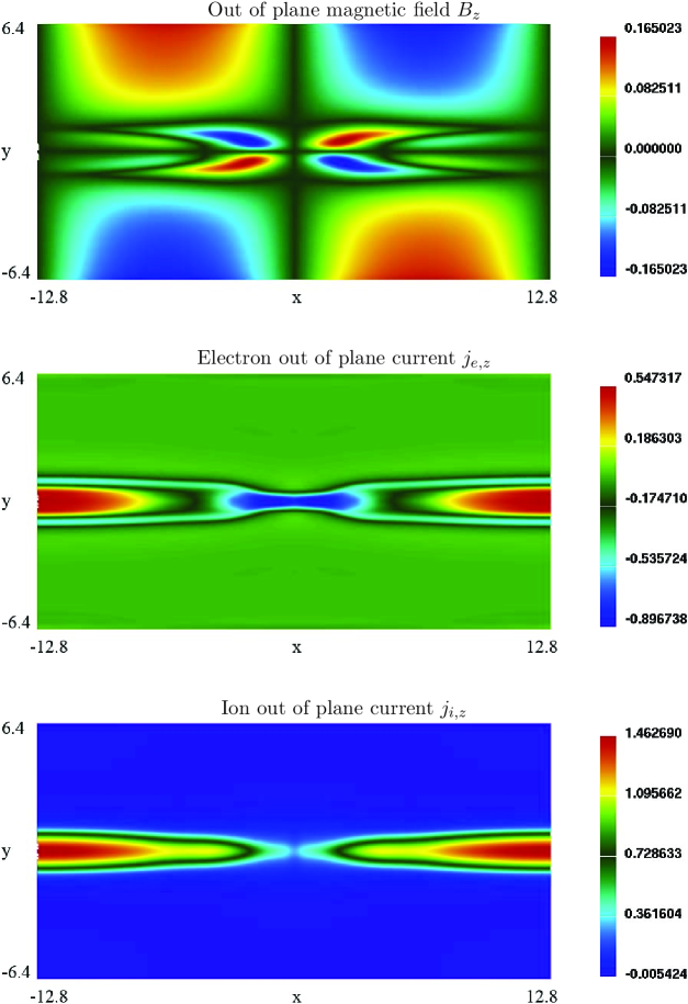
Figure 2: The out of plane magnetic field $B_{z}$ (upper panel), the electron out of plane current $j_{e,z}$ (middle panel) and the ion out of plane current $j_{i,z}$ (lower panel) at time $\Omega_{i}t=17.7$

The middle and lower panel of Figure 2 show the electron and ion out of plane current densities $j_{e,z}$ and $j_{i,z}$ at $\Omega_{i}t=17.7$. While the ion current density almost exactly follows the ion number density $n_{i}$, the electron current density is strongly enhanced near the X–line where the number densities are depleted. The thickness of the electron current layer is smaller than the ion skin depth but larger than the electron skin depth. The size is determined by the meandering motion of the electrons around the neutral line. In addition to this current sheet, we can observe thin current layers emanating from the X–line which run along the separatrix. These structures have not been reported in previous PIC simulations but can be seen in Hall–MHD simulations. Shay:01 We point out again that the mass ratio in the GEM simulations was fixed at $m_{i}/m_{e}=25$ for both PIC Shay:01 ; Pritchett:2001b ; Hesse:2001 and hybrid Shay:01 ; Kuznetsova:2001 simulations. The difference between the Vlasov code and the PIC code, therefore, can only be explained by the differences in the numerical approach.

Figure 3: Velocity profile at $\Omega_{i}t=18.1$ as a function of $x$ at the location of the current sheet $z=0$ for electrons and ions.

The electron and ion bulk velocity profiles $v_{x}(x)$ along the direction of the current sheet are shown in Figure 3. One can see that the electrons are ejected away from the X–line at super–Alfvénic speeds. These velocity profiles are almost identical to those reported in Ref. Pritchett:2001b, . In contrast to those results, no averaging over a finite time period had to be carried out here because the Vlasov simulations do not suffer from artificial numerical noise.

IV.1 Ohm’s Law

Within the GEM reconnection challenge it has become clear that the Hall–MHD model is a minimal model to understand collisionless reconnection. Shay:01 In Hall–MHD Ohm’s law has the form

$$\frac{m}{ne^{2}}\frac{dj}{dt}=\mathbf{E}+\mathbf{v_{i}}\times\mathbf{B}-\frac{1}{ne}\mathbf{j}\times\mathbf{B}+\frac{1}{ne}\nabla\cdot\underline{\mathbf{P}}_{e},$$

where the resistivity has been neglected. This is the exact electron momentum equation which can be derived from kinetic theory of a collisionless plasma without any approximations. At large scale lengths only the MHD terms play a role, while the Hall term and the electron pressure gradient can be neglected. To investigate the regions in which the terms of the generalized Ohm’s law become important, we calculated the different contributions in the whole reconnection region.

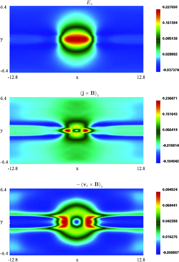
Figure 4: $z$–component of the inductive electric field $E_{z}$ (upper panel), Hall Term $\mathbf{j}\times\mathbf{B}$ (middle panel) and the negative $z$–component of $\mathbf{v}_{i}\times\mathbf{B}$ (lower panel) at time $\Omega_{i}t=17.7$

The top panel of Figure 4 shows the inductive electric field $E_{z}$. This inductive field is necessary for reconnection to take place. The region of enhanced $E_{z}$ is situated in a relatively large region around the X–line. The peak electric field is located in an elongated area extending about two ion inertial lengths in the $y$–direction and about 4 ion inertial lengths in the $x$–direction. In contrast, the region where the field exceeds half its peak value is almost circular with a diameter of about 5 ion inertial lengths. The middle panel of Figure 4 shows the $z$–component of the Hall term $\left(\mathbf{j}\times\mathbf{B}\right)_{z}$. In contrast to the inductive electric field, this quantity shows a more detailed structure. Two strong peaks are found left and right of the X–line. The peak values slightly exceed the maximum value of $E_{z}$. These peaks coincide with the maxima of the electron outflow velocity (see Figure 3). This shows that the Hall term is most important in the outflow regions where the electrons are accelerated to super Alfvénic velocities. In addition, two weaker peaks are located above and below the X–line, where the electrons are accelerated towards the X–line and the electron velocity starts to diverge from the $\mathbf{E}\times\mathbf{B}$–velocity. Due to the symmetry conditions, the Hall–term is exactly zero at the X–line itself. In addition to the structure around the X–line, we also observe sheets of negative valued Hall–term along the separatrix. We attribute this to the current loop that generates the quadrupolar magnetic field $B_{z}$. Away from the X–line, the electrons responsible for the current have to cross the separatrix back into the upstream region in order to close the loop. Therefore, the Hall–term will have negative values along the separatrix. The magnitude of the Hall–term here is almost half the peak magnitude in the X–line region.

The bottom panel of Figure 4 shows the distribution of $-\left(\mathbf{v}_{i}\times\mathbf{B}\right)_{z}$. This term becomes non–zero when ions can move across the magnetic field lines in a region of a few ion inertial lengths around the X–line. Again two peaks can be observed in the outflow region. The peak values are, however, less than half of the inductive electric field. A striking feature in this picture is the almost circular ring around the X–line, where the ions become demagnetized. The sheets of enhanced value along the separatrix are narrower than those observed from the Hall–term. They have the same sign as the peaks near the X–line and therefore partially cancel the Hall–term.

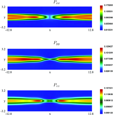
Figure 5: The diagonal components of the pressure tensor at time $\Omega_{i}t=17.7$

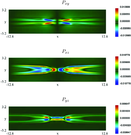
Figure 6: The off–diagonal components of the pressure tensor at time $\Omega_{i}t=17.7$

Figures 5 and 6 display the components of the electron pressure tensor. Although only the two mixed elements $P_{xz}$ and $P_{yz}$ play a role in the $z$–component of Ohm’s law, the other elements are shown for completeness. The upper panel of Figure 5 shows the diagonal terms of the pressure tensor. Here we see the differences in the heating of the electrons in the three directions. In all three cases the maximum is reached in the outflow region, where the electron velocities are super Alfvénic. The heating in the x–direction, which is mainly parallel to the magnetic field lines, is strongest. $P_{xx}$ is increased mostly in the outflow region, with only a slight increase in the diffusion region. In the outflow region $P_{yy}$ and $P_{zz}$ are comparable, because these two directions are roughly perpendicular to the magnetic field lines. Within the diffusion region $P_{yy}$ and $P_{zz}$ are, however, different. While $P_{yy}$ is enhanced in a narrowing X type region, $P_{zz}$ shows a bar like structure. The reason for this structure of $P_{zz}$ may be seen in the acceleration of a part of the electron population in the $z$–direction. This will become more apparent in the next section, where the electron distributions are investigated in detail.

The off–diagonal elements of the pressure tensor are shown in Figure 6. The magnitude of these is roughly one order of magnitude smaller than the diagonal elements which agrees remarkably well with the results of Kuznetsova et al. Kuznetsova:2001 The $P_{xy}$ component (top panel) shows a quadrupolar structure similar to the out out plane magnetic field $B_{z}$. The $P_{xz}$ component has two extrema left and right of the X–line at the edges of the diffusion region in agreement with Ref. Kuznetsova:2001, . In addition, we find two more extrema along the $y=0$ line in the electron acceleration region and also enhanced values around the separatrix. Finally, $P_{yz}$ shows a double bar structure in the diffusion region and also extrema are found in the electron acceleration region.

Figure 7: Inductive electric field $E_{z}$ at the X–line over time together with the contributions $\partial P_{xz}/\partial x$ and $\partial P_{yz}/\partial y$ from the pressure tensor.

The terms of the pressure tensor that contribute at the X–line $x=y=0$ are given by $\partial P_{xz}/\partial x$ and $\partial P_{yz}/\partial y$. In Figure 7 we have plotted the inductive electric field $E_{z}$ at the X–line over time together with the two gradients of the off–diagonal elements of the pressure tensor. We can clearly observe that the two contributions $\partial P_{xz}/\partial x$ and $\partial P_{yz}/\partial y$ are roughly equal. The sum of the two shows are remarkable agreement with the electric field over the whole time of the simulation. This indicates that, at the X–line, the bulk inertia plays only a minor role. The bulk inertia scales like $\lambda_{e}/L$ (see Ref. Vasyliunas:1975, ), where $\lambda_{e}$ is the electron inertial length and $L$ is a typical gradient scale length. Around the zero line of the magnetic field, the scale lengths of the electron dynamics are given not by the electron inertial lengths, but by the larger scale of the meandering electron motion. Speiser:1991 ; Horiuchi:1997 ; Kuznetsova:1998 For this reason, the contribution of the non–gyrotropic pressure exceeds the bulk electron inertia. For more realistic mass ratios we expect the electron bulk inertia to be completely negligible. The pressure terms should, on the other hand, remain important also for higher mass ratios. Note that the importance of the non–gyrotropic pressure has been shown only close to the X–line. Away from the X–line, but still inside the diffusion region, we find the Hall–term $\mathbf{j}\times\mathbf{B}$ to play a dominant role.

IV.2 Electron distribution function

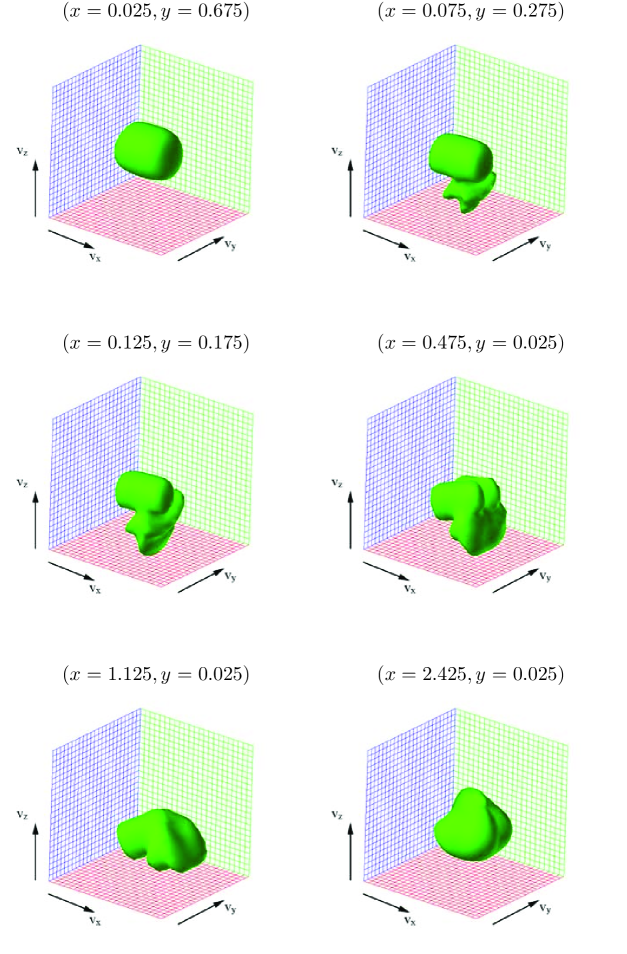
Figure 8: Isosurface of the electron distribution function in velocity space for different positions in the simulation box. The red plane is $v_{z}=$const, the blue plane is $v_{x}=$const and the green plane is $v_{y}=$const. The isosurface is drawn at $f_{e}(v_{x},v_{y},v_{z})=f_{max}/2$ where $f_{max}=f_{max}(x,y)$ if the maximum value of the distribution function at the position (x,y). The velocity box ranges from $v_{k}=$-3.67 to 3.67 for all three velocity components.

To analyze the kinetic mechanism that is responsible for the generation of the non–gyrotropic electron pressure, we have to look at the structure of the electron distribution functions in the vicinity of the X–line. Figure 8 shows isosurface plots of $f_{e}(\mathbf{x},\mathbf{v})$ in velocity space for various fixed positions $(x,y)$ in the simulation box. The sequence of sample points are chosen to follow a path from inflow region, just outside the diffusion region, through the diffusion region and to a point in the outflow region. The first panel shows the distribution function at $(x,y)=(0.025,0.675)$. This is close to the symmetry axis $x=0$ and in the inflow region, just outside the diffusion region. Note that the points could not be chosen to lie on the lines of symmetry ($x=0$ or $y=0$) since these were between the grid points in configuration space. Here the distribution function is slightly elongated in the $x$–direction indicating a slightly larger pressure $P_{xx}>P_{yy},P_{zz}$ at this point. This moderate increase in $P_{xx}$ can also be observed in Figure 5. While $P_{yy}$ and $P_{zz}$ exhibit a sharp increase at the inflow edge of the diffusion region, $P_{xx}$ rises more gradually. The distribution at this point is totally made up of the background electron population. The point $(x,y)=(0.075,0.275)$ lies just inside the diffusion region. In addition to the original background population, here two new electron populations suddenly appear. Both of these have a negative $v_{z}$–velocity. The first population is elongated in $v_{x}$ and $v_{y}$ direction. It is slightly bent which indicates a gyro motion. We interpret this population as being the background electrons originating from the other side of the current sheet. These electrons move through the magnetic zero line and show a bunched gyro motion when they enter the region on the other side with the oppositely directed magnetic field. Finally the second new electron population shows a sharp distribution with a strong negative $v_{z}$–velocity. These are the electrons which have been accelerated in the diffusion region.

In the left panel on the middle row of Figure 8 the sample point $(x,y)=(0.125,0.175)$ has moved closer to the $y=0$ line of symmetry but away from the $x=0$ line of symmetry. Here the populations already seen in the last panel become more pronounced. The gyration of the electrons from the opposite side of the current is now more apparent. This population has a distribution which exhibits a banana like shape, bent around the $v_{x}$–axis. This indicates a bunched gyro–motion. In addition, the distribution has been stretched to even higher negative $v_{z}$–velocities. An slight asymmetry can be seen in the $v_{x}$–direction due to the onsetting acceleration towards the outflow region. As one moves away from the $x=0$ line of symmetry towards larger values of $x$, one must distinguish between those electrons flowing into the diffusion region from the $\pm y$–directions and those electrons that have entered the diffusion region closer to the X–line. The latter population already has a strong directed velocity in the outflow direction. This can be seen in the right panel on the middle row which displays the distribution at $(x,y)=(0.475,0.025)$. This position is almost on the $y=0$ line of symmetry. Again the points could not be chosen to exactly lie on the line of symmetry because of the choice of the numerical grid. In this panel, the two populations from the $\pm y$–directions can be identified as two elongated blobs lying parallel to each other. The fact that these two blobs are well separated indicates that their relative velocity is larger than the thermal velocity of the electrons. For realistic mass ratios the theral velocity of the electrons will increase and the structure of the distribution function will be smeared out. Nevertheless, we expect the underlying mechanisms of meandering motion and acceleration in the $z$–direction to remain unchanged. The other population, which has already spent more time in the diffusion region, has been accelerated toward the outflow region. Both, the blobs and the accelerated population appear slightly tilted around the $v_{y}$ axis. This could indicate a gyro–motion around the newly reconnected magnetic field in the $y$–direction. In the bottom–left panel, $(x,y)=(1.125,0.025)$, this rotation is even more pronounced. Here the different populations start to merge and lose their individual identity. Finally at $(x,y)=(2.425,0.025)$ (bottom–right panel) most of the structure has been lost. The temperature has risen considerably and a directed velocity in the $v_{x}$–direction is observed.

The strongly structured electron distribution function is responsible for the off-diagonal terms of the electron pressure tensor. The structuring is due to the meandering motion of the electrons in the region where the magnetic field approaches zero and changes sign. Horiuchi:1994 ; Horiuchi:1997 The distribution function is made up of a number of distinguishable populations, which have a relative velocity, which is higher than the thermal velocity.

V Summary and Conclusions

Two and a half dimensional Vlasov simulations were carried out on the GEM magnetic reconnection setup. Vlasov codes have the advantage, with respect to PIC codes, that they do not suffer from numerical noise and that the distribution function can be analyzed with high accuracy. This advantage is gained at the cost of a substantially higher computational effort. We could reproduce the results of other kinetic simulations carried out of the GEM setup Pritchett:2001b but were also able to calculate the terms in Ohm’s law, especially the contributions from the electron pressure tensor. This shows that, although computationally more expensive, Vlasov–codes are a valuable tool for investigating collisionless reconnection. The large scale structure of the magnetic field and the electron and ion current densities agreed well with particle simulations. Pritchett:2001b In addition we were able to identify some small scale structures of the electron current density which showed enhanced values along the separatrix. While these structures were probably smeared out in PIC simulations due to the numerical noise, they resemble more the results seen in hybrid models. Shay:01 ; Kuznetsova:2001

The analysis of the contributions to the inductive electric field in Ohm’s law show that, due to the evolution of the reconnection on ion timescales rather than electron timescales, the bulk inertia of the electron plays a minor role. The effect of the bulk inertia will be decreased even more, if more realistic mass ratios are used. We could show that the Hall–term dominates at the inflow and the outflow edges of the diffusion region. Symmetry constraints, however, cause the Hall term and the $\mathbf{v}_{i}\times B$–term to vanish at the X–line. Here we could confirm the importance of the non–gyrotropic pressure, which was previously investigated by Kuznetsova et al. Kuznetsova:1998 ; Kuznetsova:2001 The evaluation of the gradients of the off–diagonal pressure components throughout the whole time showed, that both $\partial P_{xz}/\partial x$ and $\partial P_{yz}/\partial y$ contribute roughly the same towards the electric field. The sum of the two contributions could explain almost the complete inductive electric field at the X–line.

The kinetic mechanisms responsible for the non–gyrotropic electron pressure were uncovered by investigating the electron distribution function. The meandering motion of the electrons in the region of the zero magnetic field is believed to be associated with the non–gyrotropic pressure. Speiser:1991 ; Horiuchi:1994 ; Horiuchi:1997 The complex structure of the electron distribution function showed that the meandering motion is responsible. For the GEM parameters it is, however, not caused by the thermal electron motion but by the directed velocity gained in the inflow. This may, of course, be the result of the relatively high electron mass. In simulations with more realistic mass ratios we expect the inflow velocity to be considerably smaller than the thermal velocity of the electrons.

References

- (1) E. N. Parker, J. Geophys. Res. 62, 509 (1957).
- (2) P. A. Sweet, The neutral point theory of solar flares, in Electromagnetic Phenomena in Cosmical Physics, edited by B. Lehnert, (Cambridge Univ. Press, 1958) page 123
- (3) D. Biskamp, Phys. Fluids 29, 1520 (1986).
- (4) M. A. Shay, J. F. Drake, B. N. Rogers, and R. E. Denton, J. Geophys. Res. 106, 3759 (2001).
- (5) R. F. Lottermoser and M. Scholer, J. Geophys. Res. 102, 4875 (1997).
- (6) X. Wang, A. Bhattacharjee, and Z. W. Ma, Phys. Rev. Lett. 87, 265003 (2001).
- (7) J. D. Huba and L. I. Rudakov, Phys. Rev. Lett. 93, 175003 (2004).
- (8) J. Birn and M. Hesse, J. Geophys. Res. 106, 3737 (2001).
- (9) A. Otto, J. Geophys. Res. 106, 3751 (2001).
- (10) Z. W. Ma and A. Bhattacharjee, J. Geophys. Res. 106, 3773 (2001).
- (11) M. M. Kuznetsova and M. Hesse, J. Geophys. Res. 106, 3799 (2001).
- (12) P. L. Pritchett, J. Geophys. Res. 106, 3783 (2001).
- (13) M. Hesse, J. Birn, and M. Kuznetsova, J. Geophys. Res. 106, 3721 (2001).
- (14) J. Birn et al., J. Geophys. Res. 106, 3715 (2001).
- (15) M. M. Kuznetsova, M. Hesse, and D. Winske, J. Geophys. Res. 103, 199 (1998).
- (16) V. M. Vasyliunas, Rev. Geophys. 13, 303 (1975).
- (17) J. W. Dungey, Noise–free neutral sheets, in Reconnection in Space Plasmas, edited by T. D. Guyenne and J. J. Hunt (Eur. Space Agency Spec. ESA, 1988) vol 15, page SP-285.
- (18) M. Hesse and D. Winske, J. Geophys. Res. 20, 1207 (1993).
- (19) T. W. Speiser, P. B. Dusenbery, R. F. M. Jr, and D. J. Williams, Particle orbits in magnetospheric current sheets: Accelerated flows, neutral line signature and transitions to chaos, in Modeling Magnetospheric Plasma Processes, edited by G. R. Wilson (AGU, Washington D.C., 1991), vol 62 of Geophys. Monogr. Ser., page 71.
- (20) C. K. Birdsall and A. B. Langdon, Plasma Physics via Computer Simulation, (McGraw-Hill, New York, 1985).
- (21) H. Schmitz and R. Grauer, J. Comp. Phys. 214, 738 (2006).
- (22) F. Filbet, E. Sonnendrücker, and P. Bertrand, JCP 172, 166 (2001).
- (23) H. Schmitz and R. Grauer, Comput. Phys. Commun. 175, 86 (2006),
- (24) E. G. Harris, Il Nuovo Cimento 23, 115 (1962).
- (25) B. U. Ö. Sonnerup, Magnetic field reconnection, in Solar System Plasma Physics, edited by L. T. Lanzerotti, C. F. Kennel, and E. N. Parker (North–Holland Pub., New York, 1979), volume III, page 45.
- (26) T. Terasawa, Geophys. Res. Lett. 10, 475 (1983).
- (27) R. Horiuchi and T. Sato, Phys. Plasmas 4, 277 (1997).
- (28) R. Horiuchi and T. Sato, Phys. Plasmas 1, 3587 (1994).