Relaxation in statistical many-agent economy models

Abstract

We review some statistical many-agent models of economic and social systems inspired by microscopic molecular models and discuss their stochastic interpretation. We apply these models to wealth exchange in economics and study how the relaxation process depends on the parameters of the system, in particular on the saving propensities that define and diversify the agent profiles.

I Introduction

One might question how theories that try to explain the physical world of elementary particles, atoms, and molecules can be applied to understand the social structure in its complexity and the economic behavior of human beings: is it possible to describe the behavior of people with simple models? Is it even possible to identify and quantify the nature of the interactions between them? Even though it is still difficult to find answers to these questions, during the past decade physicists have made attempts to study problems related to economics, the social science that seeks to analyze and describe the production, distribution, and consumption of wealth EB- .

Here we will not try to review all these attempts, rather we briefly describe what we name statistical many-agent models. In these models, economic activity is described as a flow of wealth between basic units, referred to as agents, representing e.g. individuals or companies. Each of the $N$ agents $\{1,\ 2,\ \dots,\ i,\ \dots,\ N\}$ has a wealth $x_{i}$, that changes in time as agents exchange wealth between each other, according to the trading rules detailed in Sec. II. These underlying trading rules only depend on one set of parameters, namely the saving propensities $\{\lambda_{i}\}$, with $0\leq\lambda_{i}<1$. Statistical many-agent models describe closed economy systems and can reproduce some features of wealth distributions, such as an exponential at intermediate values of wealth and a power law at high values. In a particular model, all agents have the same global $\lambda$; in a more general model, different agents have different values of $\lambda$.

If the saving propensity is equal for all the units (global saving propensity models), $\lambda_{i}\equiv\lambda$, the equilibrium wealth density $f(x)$ is given by a $\Gamma$-distribution,

$$f(x) = \beta\,\gamma_{n}(\beta x)=\frac{\beta}{\Gamma(n)}\,(\beta x)^{n-1}\exp(-\beta x)\,,$$ (1)

$$n = \frac{D}{2}=\frac{1+2\lambda}{1-\lambda}\,.$$ (2)

Here $n$ is a real number in the interval $[1,\infty)$ and $D=2n$ can be considered as the effective dimension of the system: in fact the distribution $\gamma_{n}(\beta x)$ is just the Maxwell-Boltzmann distribution for the kinetic energy $x$ of a gas in thermal equilibrium at a temperature $\beta^{-1}$ in a $D$-dimensional space. Thus the parameter $\beta$ can be interpreted as the inverse temperature: consistently with the equipartition theorem, $\beta^{-1}=2\langle x\rangle/D=\langle x\rangle/n$, where the constant $\langle x\rangle$ is the average wealth $\langle x\rangle=X/N$ and $X=\sum_{i=1}^{N}x_{i}$ is the total wealth. In an economic system, temperature is proportional to the fluctuations of wealth around its average value. The model with a single global saving propensity describes well wealth distributions at intermediate values of $x$, but cannot predict power laws at large $x$.

If $\lambda$ is uniformly distributed among the agents according to a given density $\phi(\lambda)$ (distributed saving propensity models), then one finds, under quite general conditions on the shape of $\phi(\lambda)$, an exponential law at intermediate values of $x$ and a robust Pareto law,

$$f(x)\propto x^{-1-\alpha},$$ (3)

with $\alpha\geq 1$, at large $x$. This power law was suggested by Vilfredo Pareto Pareto (1897) more than a century ago to describe the tail of wealth distributions and is usually found to be characterized across various countries by a Pareto exponent $\alpha\approx 3/2$.

The basic exchange laws underlying some of these models are reviewed in Sec. II. In Sec. III we focus on the relaxation to equilibrium generated by the exchange laws of models with uniformly distributed $\lambda$ and illustrate its dependence on the saving propensity $\lambda$ through some examples. We also consider the corresponding relaxation time distributions and discuss the relation between the Pareto exponent and the relaxation behavior of the system. Results are summarized in Sec. IV.

II Many-agent models of a closed pure exchange economy

Our aim is to study a general many-agent statistical model of a closed economy without growth (analogous to the kinetic theory model of ideal gases, see Fig. 1), where $N$ agents exchange a quantity $x$, that we have defined as wealth. The states of the agents are specified only by the wealths $\{x_{i}\}$, while the total wealth $X=\sum_{i=1}^{N}x_{i}$ is conserved. The evolution of the system is carried out according to the following algorithm: at every time step two agents $i$ and $j$ are chosen randomly and an amount of wealth $\Delta x$ is exchanged, so that the agent wealths $x_{i}^{\prime}$ and $x_{j}^{\prime}$ after the transaction are

$$x_{i}^{\prime} = x_{i}-\Delta x\,,$$

$$x_{j}^{\prime} = x_{j}+\Delta x\,.$$ (4)

Different transaction rules have been studied analytically or numerically by various authors and are summarized here below.

II.1 Basic model without saving: Boltzmann distribution

A stochastic trading rule, that redistributes the wealths of two agents randomly, was introduced in Ref. Dragulescu and Yakovenko, 2000,

$$x_{i}^{\prime} = \epsilon(x_{i}+x_{j})\,,$$

$$x_{j}^{\prime} = \bar{\epsilon}(x_{i}+x_{j})\,,$$ (5)

where $\epsilon$ is a uniform random number in $(0,1)$ and $\epsilon+\bar{\epsilon}=1$. Eqs. (II.1) are equivalent to the trading rule of Eq. (II) if $\Delta x=\bar{\epsilon}x_{i}-\epsilon x_{j}$. In another version of the model, the money difference $\Delta x$ is assumed to have a constant value independent of the two trading agents Bennati (1988a, b, 1993), i.e. $\Delta x=\Delta x_{0}$. Both these forms for $\Delta x$ lead to a robust equilibrium Boltzmann (or Gibbs) distribution,

$$f(x)=\beta^{-1}\exp(-\beta x)\,,$$ (6)

with effective temperature $\beta^{-1}=\langle x\rangle=X/N$ Dragulescu and Yakovenko (2000); Bennati (1988a, b, 1993).

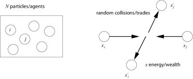
Figure 1: Analogy between the minimal closed pure exchange economic model and a classical isolated system of an ideal gas. In the latter case particles undergo random elastic collisions and exchange a fraction of their kinetic energy, while in the closed economy model agents perform random trades with each other and exchange a fraction of their wealth according to some statistical rule.

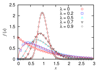
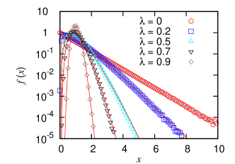
Figure 2: Wealth probability density in linear (left) and semi-log (right) scale for various global saving propensities $\lambda$. The exponential curve $\lambda=0$ is the equilibrium solution for the basic model (Sec. II.1), while the other curves correspond to a nonzero global saving propensity (Sec. II.2).

II.2 Model with a global saving propensity: Gamma distribution

Introducing a saving criterion through a saving propensity parameter $0\leq\lambda<1$ Chakraborti and Chakrabarti (2000); Chakraborti (2002) modifies the trading rule as follows:

$$x_{i}^{\prime} = \lambda x_{i}+\epsilon(1-\lambda)(x_{i}+x_{j})\,,$$

$$x_{j}^{\prime} = \lambda x_{j}+\bar{\epsilon}(1-\lambda)(x_{i}+x_{j})\,.$$ (7)

This model is similar to that introduced by John Angle in 1983 on the basis of the Surplus Theory Angle (1983, 1986, 2006), which however differs both in the mathematical definition of the exchange rule and interpretation Angle (2006). A closer comparison will be studied elsewhere, while here, for the sake of simplicity, we will focus on the trading rule (II.2) and some of its generalizations for studying the relaxation process. The rule of Eq. (II.2) corresponds to the process defined by Eq. (II) if

$$\Delta x=(1-\lambda)(\bar{\epsilon}x_{i}-\epsilon x_{j})\,.$$ (8)

The parameter $\lambda$ represents the fraction of wealth saved before the reshuffling takes place. The resulting equilibrium distribution is qualitatively different from a simple exponential function, being a $\Gamma$-distribution Patriarca et al. (2004a, b), see Eq. (1), that has a mode $x_{m}>0$ and a zero limit for $x\to 0$, see Fig. 2.

II.3 Models with a continuous distribution of saving propensities

More realistic and interesting models are obtained when agents $i=1,\ \dots,\ N$ are diversified by assigning them different saving propensities $\lambda_{i}$ Angle (2002); Chatterjee et al. (2003); Das and Yarlagadda ; Chatterjee et al. (2004); Repetowicz et al. (2005); Chatterjee et al. (2005); Das and Yarlagadda (2005); Patriarca et al. (2005), e.g. with the $\lambda_{i}$ distributed uniformly on the interval $[0,1)$. The trading rule is then

$$x_{i}^{\prime} = \lambda_{i}x_{i}+\epsilon[(1-\lambda_{i})x_{i}+(1-\lambda_{j})x_{j}]\,,$$

$$x_{j}^{\prime} = \lambda_{j}x_{j}+\bar{\epsilon}[(1-\lambda_{i})x_{i}+(1-\lambda_{j})x_{j}]\,,$$ (9)

or, equivalently, can be formulated through Eq. (II) with $\Delta x$ given by

$$\Delta x=\bar{\epsilon}(1-\lambda_{i})x_{i}-\epsilon(1-\lambda_{j})x_{j}\,.$$ (10)

Numerical simulations and theoretical considerations suggest that these models relax toward a robust power law $\propto 1/x^{1+\alpha}$ with a Pareto exponent $\alpha=1$ in the case of uniformly distributed $\lambda$ and with $\alpha>1$ if the $\lambda$-density $\phi(\lambda)\to 0$ as $\phi(\lambda)\sim(1-\lambda)^{\alpha-1}$ for $\lambda\to 1$. In the following we study the relaxation process of models with uniformly distributed $\lambda$.

III Relaxation process

If a real economic system is characterized by a wealth distribution with a certain shape, it is of great interest to know on which time scale the system relaxes toward this distribution from a given arbitrary initial distribution of wealth, and how the relaxation process depends on the system parameters, in particular on the system size and the distribution of saving propensities.

In the simulations presented below, all agents start from the same initial wealth $x_{i}(t=0)=x_{0}=1$. The value $x_{0}$, due to the conservation of the total wealth $X=\sum_{i=1}^{N}x_{i}$, also represents the global average value of $x$ at any time $t$, i.e. $\langle x(t)\rangle\equiv\int xf(x)\,dx=x_{0}=X/N$. This setup is used to model a more general situation where the initial conditions of the agents are far from equilibrium.

III.1 Relaxation to equilibrium as a function of system size

Before analyzing the dependence of the time scale on the saving propensity distribution, we shortly consider its dependence on the number of agents $N$. If time is measured by the number of transactions $T$, we find that the time scale is proportional to the number of agents $N$: a system A that is $m$ times larger than a system B ($N_{\mathrm{A}}=mN_{\mathrm{B}}$) relaxes $m$ times slower than B. This is shown in Fig. 3, where the average wealth $\langle x(t)\rangle_{\lambda}$ of the agent subset with $\lambda=0.99$ is plotted for various systems with different values of $N$ versus the rescaled time $t=T/N$. However, the $\lambda$-density $\phi(\lambda)$ is the same for all systems and uniformly partitions each system into $100$ subsets with values $\lambda=0.00,\ 0.01,\ \dots,\ 0.99$.

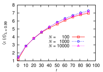
Figure 3: Average wealth $\langle x(t)\rangle_{\lambda=0.99}$ versus the rescaled time $t=T/N$ for systems with different number of agents $N=100$, $1000$, and $10\,000$, but the same saving propensity density $\phi(\lambda)$, that uniformly partitions agents into $100$ subsets with $\lambda=0.00,\ 0.01,\ \dots,\ 0.99$. $T$ is the total number of trades.

Here and in the following we define time $t$ as the ratio $t=T/N$ between the total number of trades $T$ and the total number of agents $N$, i.e. what is usually called a Monte Carlo cycle or sweep in molecular simulation Allen and Tildesley (1989): in a Monte Carlo cycle, each agent performs on average the same number of trades (actually two), in the same fashion as in molecular dynamics each particle is moved once at every time step. The results will not change if one of the two agents involved in an exchange is selected sequentially, e.g. in the order of its index $i=1,\ \dots,\ N$, as is common practice in molecular simulations. This ensures that every agent performs at least one trade per cycle and reduces the amount of random numbers to be drawn. The previous considerations suggest the introduction of a time unit $\tau_{0}$, such that during any time interval $(t,t+\tau_{0})$ all agents perform on average one trade (or the same number of trades). In this way the dynamics and the relaxation process become independent of $N$. The existence of a natural time scale independent of the system size provides a foundation for using simulations of systems with finite $N$ in order to infer properties of systems with continuous saving propensity distributions and $N\to\infty$.

III.2 Relaxation to equilibrium as a function of saving propensity

Relaxation in systems with constant $\lambda$ has already been studied in Ref. Chakraborti and Chakrabarti, 2000, where a systematic increase of the relaxation time with $\lambda$, and eventually a divergence for $\lambda\to 1$, was found: for $\lambda=1$, no exchanges can occur, so that the system is frozen. Here we consider systems with uniformly distributed $\lambda$. In this case a similar behavior of the relaxation times is observed, broken down to subsystems with similar values of $\lambda$. As discussed in detail in Refs. Patriarca et al., 2005; Bhattacharya et al., 2005; Patriarca et al., 2006, the partial wealth distributions of agents with a given value of $\lambda$ relax toward different states with characteristic shapes $f_{\lambda}(x)$. The generic function $f_{\lambda}(x)$ has a maximum and an exponential tail, thus closely recalling the shape of a $\Gamma$-distribution. The corresponding average value is given by $\langle x\rangle_{\lambda}\equiv\int xf_{\lambda}(x)\,dx=k/(1-\lambda)$, where $k$ is a suitable constant determined through the condition $\int\langle x\rangle_{\lambda}\,\phi(\lambda)\,d\lambda=X/N$; $X$ is the total wealth of the system. Even if the partial distributions decay exponentially with $x$, the sum of all partial distributions results in a Pareto law at large values of $x$, i.e. $f(x)=\sum_{\lambda}f_{\lambda}(x)\sim 1/x^{1+\alpha}$. Numerical simulations clearly show that agents with different values of $\lambda$ are associated to different relaxation times $\tau_{\lambda}$.

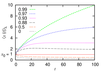
Figure 4: Mean wealth $\langle x(t)\rangle_{\lambda}$ versus time for various $\lambda$. The $10^{4}$ agents are uniformly partitioned into $100$ subsets with $\lambda=0.01,\ 0.02,\ \dots,\ 0.99$. Higher $\lambda$ correspond to longer relaxation times. The continuous line $\langle x\rangle=x_{0}$ partitions agents into poor ($x<x_{0}$) and rich ($x>x_{0}$) ones.

Results are illustrated in Fig. 4 for a system of $N=10^{4}$ agents uniformly partitioned into $100$ subsets with $\lambda=0.01,\ 0.02,\ \dots,\ 0.99$: mean wealths of subsets corresponding to a value of $\lambda$ closer to 1 relax slower toward their asymptotic average wealth $\langle x\rangle_{\lambda}\propto 1/(1-\lambda)$.

The average wealth $x_{0}$ allows to introduce a threshold that partitions the system into poor agents, with an asymptotic average wealth $\langle x(t\to\infty)\rangle_{\lambda}<x_{0}$, and rich agents with $\langle x(t\to\infty)\rangle_{\lambda}>x_{0}$. The poor-rich threshold $\langle x\rangle=x_{0}=1$ is represented as a continuous line in Fig. 4 and corresponds to $\lambda\approx 0.75$ for this particular example.

The differences in the relaxation process can be related to the different relative wealth exchange rates, that by direct inspection of Eqs. (II.3) and (10) appear to be proportional to $1-\lambda$. Thus, in general, higher saving propensities are expected to be associated to slower relaxation processes. A more detailed analysis can be carried out as shown in Fig. 5: after the rescaling of time and wealth by the factor $(1-\lambda)$, mean wealths corresponding to agents with different values of $\lambda$ (Fig. 5 left) appear to relax approximately on the same time scale and toward the same asymptotic value (Fig. 5 right). In fact, the factor $(1-\lambda)$ is proportional to the wealth exchange rates and, at the same time, through the condition of stationarity, determines the equilibrium average wealth values $\langle x\rangle_{\lambda}=k/(1-\lambda)$ Patriarca et al. (2005). Agents start from the same initial condition $x_{i}(t=0)=x_{0}=1$. In this case, in order to study in greater detail the high saving propensity parameter region, that corresponds to the high relaxation time region, the system of $N=10^{4}$ agents has been uniformly partitioned into $200$ subsets with saving propensities $\lambda=0.5000,\ 0.5025,\ \dots,\ 0.9975$. Actually, this is not a uniform distribution of $\lambda$ on $[0,1)$, since $\phi(\lambda)=0$ for $\lambda<0.5$, however it does not matter because what counts is the high saving propensity parameter interval.

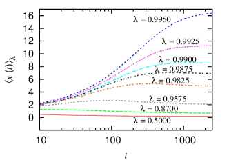
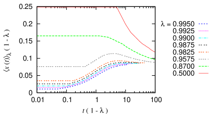
Figure 5: Left: average wealth $\langle x(t)\rangle_{\lambda}$ versus (log of) time for the $\lambda$’s listed in the figure. The $10^{4}$ agents are partitioned into $200$ subsets with $\lambda=0.5000,\ 0.5025,\ \dots,\ 0.9975$. Right: same as in the left figure after rescaling wealth and time by the factor $(1-\lambda)$, inversely proportional to the mean wealth and proportional to the average wealth exchange rate.

III.3 Relaxation time distribution

The model with distributed saving propensities is completely specified by the trading rules of Eqs. (II.3) and the set of saving propensities $\{\lambda_{i}\}$ of the $N$ agents. In the case of a continuously distributed $\lambda$, a continuous saving propensity density $\phi(\lambda)$ can be used in place of the discrete $\lambda$-set, normalized so that $\int_{0}^{1}\phi(\lambda)\,d\lambda=1$.

Here we suggest a method to obtain the wealth as well as the relaxation distribution directly from the saving propensity density $\phi(\lambda)$. It follows from probability conservation that $\tilde{f}(\bar{x})d\bar{x}=\phi(\lambda)d\lambda$, where $\bar{x}$ is a short notation for $\langle x\rangle_{\lambda}$ and $\tilde{f}(\bar{x})$ is the density of the average wealth values. In the case of uniformly distributed saving propensities, one obtains

$$\tilde{f}(\bar{x})=\phi(\lambda)\frac{d\lambda(\bar{x})}{d\bar{x}}=\phi\left(1-\frac{k}{\bar{x}}\right)\frac{k}{\bar{x}^{2}}\,.$$ (11)

This shows that a uniform saving propensity distribution leads to a power law $\tilde{f}(\bar{x})\sim 1/\bar{x}^{2}$ in the (average) wealth distribution. In general a $\lambda$-density going to zero for $\lambda\to 1$ as $\phi(\lambda)\propto(1-\lambda)^{\alpha-1}$ (with $\alpha\geq 1$) leads to the Pareto law $\tilde{f}(\bar{x})\sim 1/\bar{x}^{1+\alpha}$ with Pareto exponent $\alpha\geq 1$ as found in real distributions.

In a very similar way it is possible to obtain straightforwardly the associated distribution of relaxation times $\psi(\tau)$ for the global relaxation process through the relation between the relaxation time $\tau_{\lambda}$ and the agent saving propensity: given that the time scale follows a relation $\tau_{\lambda}\propto 1/(1-\lambda)$, then

$$\psi(\tau)=\phi(\lambda)\frac{d\lambda(\tau)}{d\tau}\propto\phi\left(1-\frac{\tau^{\prime}}{\tau}\right)\frac{\tau^{\prime}}{\tau^{2}}\,,$$ (12)

where $\tau^{\prime}$ is a proportionality factor. Comparison with Eq. (11) shows that $\psi(\tau)$ and $\tilde{f}(\bar{x})$ are characterized by power law tails in $\tau$ and $\bar{x}$ respectively with the same Pareto exponent.

It is to be noticed, as discussed in Ref. Patriarca et al., 2005, that in the parameter region $\lambda\to 1$, from which the main contributions to the Pareto power law tail come, the widths of the generic equilibrium partial distributions $f_{\lambda}(x)$ increase more slowly than the difference between the mean values $\langle x\rangle_{\lambda^{\prime}}-\langle x\rangle_{\lambda}$ corresponding to two agents with consecutive values of the saving propensity $\lambda^{\prime}$ and $\lambda$. This implies that at equilibrium and in the tail of the distribution it is possible to resolve the mixture $\sum_{\lambda}f_{\lambda}(x)$ into its components $f_{\lambda}(x)$ and to approximate the current value of wealth $x(t)$ of a certain agent with saving propensity $\lambda$ (that is actually a stochastic process) with the corresponding average value, $\langle x\rangle_{\lambda}\approx x$, so that $\tilde{f}(x)\approx f(x)$.

Finally we notice that an ensemble with a power law distribution of relaxation times undergoes a slow relaxation process if the exponent of the relaxation time distribution is smaller than two, so that a Pareto exponent larger than two, as automatically generated by the model, seems to ensure a normal relaxation.

IV Conclusions

The relaxation process of statistical many-agent models of a closed pure exchange economy, where trading is described as a flux of wealth between different agents, has been found to be slower for agents with a larger saving propensity parameter $\lambda$, who are also the agents resulting richer at equilibrium. For a uniform $\lambda$-distribution, the relaxation time is $\tau_{\lambda}\propto 1/(1-\lambda)$. Furthermore, a smooth distribution of saving propensities leads to distributions of wealth and of relaxation times characterized by power law tails with the same Pareto exponent $\alpha\geq 1$, which ensures a fast relaxation toward equilibrium.

We also remark that if time is measured in Monte Carlo cycles, i.e. the ratio between the total number of trades and the total number of agents, so that every agent performs on average two trades during a cycle, the time evolution and the relaxation process are independent of the system size, thus providing information on arbitrarily large systems.

References

-
(1)
Encyclopædia Britannica,
URL http://www.britannica.com/ebc/article-9109547. - Pareto (1897) V. Pareto, Cours d’economie politique (Rouge, Lausanne, 1897).
- Dragulescu and Yakovenko (2000) A. Dragulescu and V. M. Yakovenko, Eur. Phys. J. B 17, 723 (2000).
- Bennati (1988a) E. Bennati, La simulazione statistica nell’analisi della distribuzione del reddito: modelli realistici e metodo di Monte Carlo (ETS Editrice, Pisa, 1988a).
- Bennati (1988b) E. Bennati, Rivista Internazionale di Scienze Economiche e Commerciali pp. 735 (1988b).
- Bennati (1993) E. Bennati, Rassegna di Lavori dell’ISCO 10, 31 (1993).
- Chakraborti and Chakrabarti (2000) A. Chakraborti and B. K. Chakrabarti, Eur. Phys. J. B 17, 167 (2000).
- Chakraborti (2002) A. Chakraborti, Int. J. Mod. Phys. C 13, 1315 (2002).
- Angle (1983) J. Angle, in Proceedings of the American Social Statistical Association, Social Statistics Section (Alexandria, VA, 1983), p. 395.
- Angle (1986) J. Angle, Social Forces 65, 293 (1986), URL http://www.jstor.org.
- Angle (2006) J. Angle, Physica A 367, 388 (2006).
- Patriarca et al. (2004a) M. Patriarca, A. Chakraborti, and K. Kaski, Phys. Rev. E 70, 016104 (2004a).
- Patriarca et al. (2004b) M. Patriarca, A. Chakraborti, and K. Kaski, Physica A 340, 334 (2004b).
- Angle (2002) J. Angle, J. Math. Sociol. 26, 217 (2002).
- Chatterjee et al. (2003) A. Chatterjee, B. K. Chakrabarti, and S. S. Manna, Physica Scripta T 106, 367 (2003).
- (16) A. Das and S. Yarlagadda, A distribution function analysis of wealth distribution, URL cond-mat/0310343.
- Chatterjee et al. (2004) A. Chatterjee, B. K. Chakrabarti, and S. S. Manna, Physica A 335, 155 (2004).
- Repetowicz et al. (2005) P. Repetowicz, S. Hutzler, and P. Richmond, Physica A 356, 641 (2005).
- Chatterjee et al. (2005) A. Chatterjee, B. K. Chakrabarti, and R. B. Stinchcombe, Phys. Rev. E 72, 026126 (2005).
- Das and Yarlagadda (2005) A. Das and S. Yarlagadda, Physica A 353, 529 (2005).
- Patriarca et al. (2005) M. Patriarca, A. Chakraborti, K. Kaski, and G. Germano, in Econophysics of Wealth Distributions, edited by A. Chatterjee, S.Yarlagadda, and B. K. Chakrabarti (Springer, 2005), p. 93, URL arXiv:physics/0504153.
- Allen and Tildesley (1989) M. P. Allen and D. J. Tildesley, Computer Simulation of Liquids (Oxford University Press, Oxford, 1989), paperback ed., p. 123.
- Bhattacharya et al. (2005) K. Bhattacharya, G. Mukherjee, and S. S. Manna, in Econophysics of Wealth Distributions, edited by A. Chatterjee, S.Yarlagadda, and B. K. Chakrabarti (Springer, 2005), p. 111.
- Patriarca et al. (2006) M. Patriarca, A. Chakraborti, and G. Germano, Physica A 369, 723 (2006).