Directed Sub-Wavelength Imaging Using a Layered Metal-Dielectric System

Abstract

We examine some of the optical properties of a metamaterial consisting of thin layers of alternating metal and dielectric. We can model this material as a homogeneous effective medium with anisotropic dielectric permittivity. When the components of this permittivity have different signs, the behavior of the system becomes very interesting: the normally evanescent parts of a P-polarized incident field are now transmitted, and there is a preferred direction of propagation.

We show that a slab of this material can form an image with sub-wavelength details, at a position which depends on the frequency of light used. The quality of the image is affected by absorption and by the finite width of the layers; we go beyond the effective medium approximation to predict how thin the layers need to be in order to obtain subwavelength resolution.

I Introduction

An anisotropic material in which one of the components of the dielectric permittivity tensor has a different sign to the others has interesting properties. It supports the propagation of modes which would normally be evanescent, and these modes travel in a preferred direction. The propagation of evanescent modes gives us hope that an image produced by light travelling through a slab of such a material might retain a sharp profile; also, because the preferred direction depends on the ratio of the components of the permittivity tensor, it can be controlled by varying the frequency of light used.

We first look at a way of producing a metamaterial with the desired properties: by making a system of thin, alternating metal and dielectric layers. A system of this type was proposed by Ramakrishna et al. (2003) as a form of “superlens”; it improves on the original suggestion for a superlens,(Pendry, 2000) which consists of just a single layer of metal, and has recently been realised.Fang et al. (2005); Melville and Blaikie (2005)

We then look at the dispersion relation for our anisotropic material, to see why modes which would be evanescent in both the metal and the dielectric separately are able to propagate in the combined system, and why there is a preferred direction of propagation. The subwavelength details of the source are transmitted through the system because they couple to the surface plasmons (Ritchie, 1957) that exist on the boundaries between metal and dielectric; this mechanism is the basis for the current interest in metallic structures for super-resolution imaging at optical frequencies. (Pendry, 2000; Cai et al., 2005; Ono et al., 2005; Fang et al., 2005; Melville and Blaikie, 2005)

Next, we investigate the transmission properties of a slab of this material, and apply our formulae to the case of a line source. We show that we can expect to obtain a sharp image as long as the amount of absorption is not too high.

Finally, we go beyond the effective medium approximation to show the effect of the finite layer widths on the optical properties. We demonstrate that the “resolution” of the slab is limited by the width of the layers; thinner sheets mean that the description of the system using the effective medium becomes increasingly accurate, and the image quality improves.

II Layered systems

We concentrate on periodic layered systems of the form shown in figure 1.

Figure 1: System geometry. The layers are infinite in extent in the $xy$-plane.

We assume that each layer can be described by homogeneous and isotropic permittivity and permeability parameters. When the layers are sufficiently thin, we can treat the whole system as a single anisotropic medium with the dielectric permittivity(Rytov, 1955; Bergman, 1978)

$$\epsilon_{x} =\epsilon_{y}=\frac{\epsilon_{1}+\eta\epsilon_{2}}{1+\eta}$$ (1)

$$\frac{1}{\epsilon_{z}} =\frac{1}{1+\eta}\left(\frac{1}{\epsilon_{1}}+\frac{\eta}{\epsilon_{2}}\right),$$ (2)

where $\eta$ is the ratio of the two layer widths:

$$\eta=\frac{d_{2}}{d_{1}}.$$ (3)

A helpful way to see this is through the characteristic matrix formalism; (Born and Wolf, 1980) this method, which is related to that used by Rytov in the original derivation,(Rytov, 1955) is described in the appendix.

The homogenized magnetic permeability is given by expressions analogous to (1) and (2). When $\eta$ is small, the effective parameters are dominated by the first medium, while for large $\eta$, they resemble those of the second medium.

Only the ratio of the thicknesses of the two layers appears in the homogenized version, not the absolute value; however, the characterization of the material using the effective medium parameters is more accurate when both $d_{1}$ and $d_{2}$ are small.

For a layered metal-dielectric system, we can tune the response either by altering the frequency or by changing the ratio of layer thicknesses. (Yu et al., 2005) This is demonstrated by figures 2 and 3, which show the real and imaginary parts of the effective permittivity for two different thickness ratios, for a system composed of alternating layers of silver and silica.

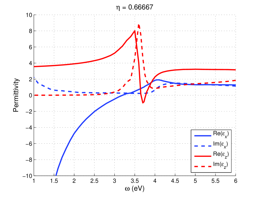
Figure 2: (Color online) The dielectric permittivity of the metamaterial constructed from layers of silver and silica. This and the following graph show the real and imaginary parts of the in-plane and perpendicular components of the permittivity for different layer thickness ratios; in this case, $\eta=2/3$, which means that the layers of silica are one and a half times as thick as the layers of metal.

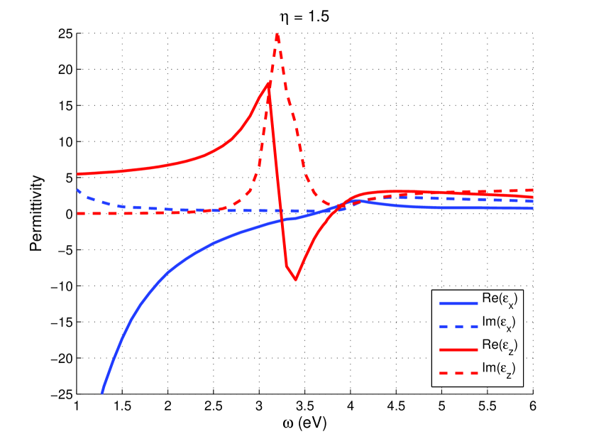
Figure 3: (Color online) The effective permittivity when $\eta=1.5$. The silver layers are now thicker, and the amount of absorption has increased: the imaginary parts of the permittivity are now larger. However, the real parts are also correspondingly larger in magnitude.

The material data from which these plots are constructed have been taken from the books by Palik (1985) and Nikogosyan (1997). In both graphs, there are two regions in which $\Re(\epsilon_{x})$ and $\Re(\epsilon_{z})$ take opposite signs. In the first region, which includes energies up to approximately 3.2 eV, $\Re(\epsilon_{x})$ is negative; in the second, which consists of a small range of energies around 3.6 eV, $\Re(\epsilon_{x})$ is positive.

By choosing a suitable value of $\eta$, we can make the real parts of $\epsilon_{z}$ and $\epsilon_{x}$ take opposite signs over a range of frequencies. We investigate the consequences of this in the next section.

III Permittivity with direction-dependent sign

The unusual behavior of the layered materials can be understood by considering the dispersion relation between the frequency $\omega$ and the wave vector ${\mathbf{k}}$. We assume that we are dealing with non-magnetic materials, so that the magnetic permeability $\mu=1$. If the dielectric permittivity is anisotropic, the interesting waves are those with transverse magnetic (TM) polarization. The dispersion relation for these waves is

$$\frac{k_{x}^{2}}{\epsilon_{z}}+\frac{k_{z}^{2}}{\epsilon_{x}}=\frac{\omega^{2}}{c^{2}}=k_{0}^{2}.$$ (4)

We have taken $k_{y}$ to be zero, since the $x$- and $y$-directions are equivalent. When $\epsilon_{x}$ and $\epsilon_{z}$ are both positive, the relationship between $k_{x}$ and $k_{z}$ is similar to that in free space: for small $k_{x}$, $k_{z}$ is real, but when $k_{x}$ becomes large, $k_{z}$ becomes imaginary. The propagation of the wave in the $z$-direction is governed by $k_{z}$; when $k_{z}$ is imaginary, the wave is evanescent: it decays exponentially with $z$.

However, when $\epsilon_{x}$ and $\epsilon_{z}$ have opposite signs, $k_{z}$ is real for a much wider range of values of $k_{x}$. Even the high spatial frequency components with large $k_{x}$, which would normally be evanescent, now correspond to real values of $k_{z}$, and hence to propagating waves.

If we want to plot the dispersion relation, we have to remember that the permittivity itself is frequency-dependent. To get an idea of what the dispersion relation looks like, we can use an idealized model: we imagine a metamaterial whose layers are composed of equal thicknesses of a dielectric, with positive, frequency-independent permittivity, and a metal, with the simple plasma-like permittivity

$$\epsilon_{\mathrm{m}}(\omega)=\epsilon_{\mathrm{m}}(\infty)-\frac{\omega_{\mathrm{p}}^{2}}{\omega^{2}}.$$ (5)

For now, we assume that the materials are non-absorbing. The resulting dispersion relation is plotted in figure 4.

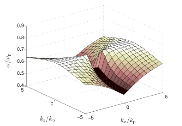
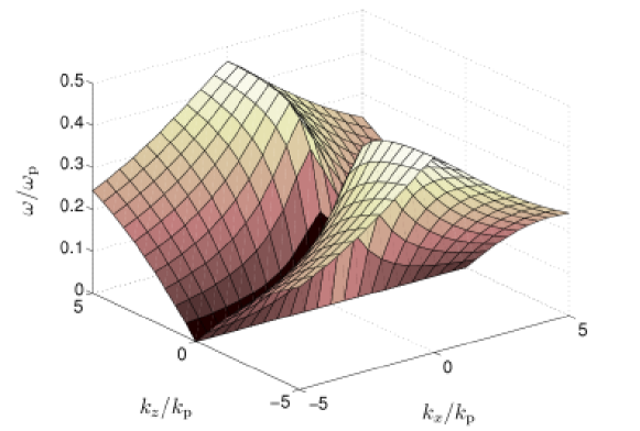
Figure 4: (Color online) The dispersion relation for an idealized metal-insulator system. The permittivity of the metal is given by (5) with $\epsilon_{\mathrm{m}}(\infty)=2.0$, while the dielectric has permittivity $\epsilon_{\mathrm{d}}=2.5$; the layers are of equal width ($\eta=1$). $k_{\mathrm{p}}$ is the wave vector corresponding to the plasma frequency ($k_{\mathrm{p}}=\omega_{\mathrm{p}}/c$). The first two bands are shown; they have been separated to make visualisation easier, but there is no band gap. The plots are symmetric about the planes $k_{x}=0$ and $k_{z}=0$.

We can identify two distinct bands from the figure. In the lower, $\epsilon_{x}$ is negative, while $\epsilon_{z}$ is positive; the signs are reversed in the upper band. In both cases, the contours of constant $\omega$ are hyperbolae. In the lower band, these hyperbolae are centered on the $k_{x}$-axis, while in the upper, they are centered on the $k_{z}$-axis.

In fact, there is also a third band at high frequencies, but this is the least interesting regime and is not shown in figure 4: both components of the permittivity are positive here.

The dispersion relation also provides the key to the preferred propagation direction. This is determined by the group velocity. A constant-frequency section of the dispersion relation (cut across the first band) is plotted in figure 5.

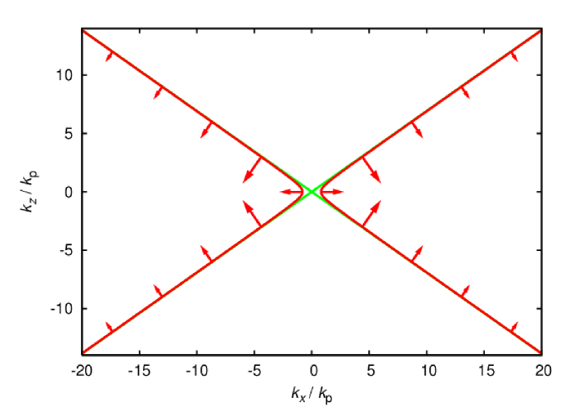
Figure 5: (Color online) The relationship between $k_{x}$ and $k_{z}$ for $\omega=0.2\omega_{\mathrm{p}}$ (in the middle of the lower band in figure 4). The straight lines show the asymptotes given by equation (6). The group velocity is indicated by the arrows, which are perpendicular to the curve; the length of the arrows is proportional to the magnitude of the group velocity.

The hyperbolic form of the curve means that for large $|k_{x}|$, it tends to the following straight line:

$$k_{z}=\sqrt{-\frac{\epsilon_{x}}{\epsilon_{z}}}|k_{x}|.$$ (6)

The group velocity is perpendicular to the constant-$\omega$ contours like the one plotted in figure 5. The figure demonstrates that apart from a region around $k_{z}=0$, the group velocity vectors all point in almost the same two directions: this is the basis for the preferred direction of propagation. Remembering that the $x$- and $y$-directions are equivalent, we can see that the preferred directions form a cone around the $z$-axis. The half-angle of the cone is

$$\theta=\arctan\sqrt{-\frac{\epsilon_{x}}{\epsilon_{z}}}.$$ (7)

In the region around $k_{z}=0$, the arrows point outside the cone. In this band, there are no propagating modes in a small region around $k_{x}=0$, and no propagating modes with a group velocity vector lying inside the cone.

If we take a cross-section from the second band, instead of the first, we also see a hyperbolic contour; the plot resembles figure 5, but rotated by 90^∘. The group velocities for the modes around $k_{x}=0$ now point inside the cone, rather than outside.

To conclude this section, we look at the physical process that allows our layered metamaterial to mimic an anisotropic material and to support the propagation of normally evanescent waves. The key fact is that surface plasmons are supported at an interface where the permittivity changes sign. When the metal permittivity is negative, this sign change occurs at every interface; the wave is transmitted via coupled surface plasmons, as indicated in figure 6.

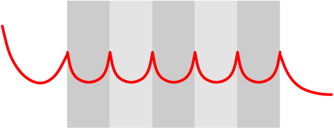
Figure 6: (Color online) Schematic diagram of the transmission of normally evanescent waves, showing the role of surface plasmons. The line represents the electric field strength.

IV Transmission through an anisotropic system

We have seen that we can produce a metamaterial with interesting properties by stacking alternating layers of metal and dielectric. Next, we look at a slab of this material, and examine the transmission coefficient.

We assume that the slab is embedded in a uniform medium of constant permittivity (which may be unity, representing vacuum). In such a medium, the dispersion relation (4) becomes

$${k_{x}^{2}}+{k_{z}^{\prime 2}}=k_{0}^{2}\epsilon.$$ (8)

We write $k_{z}^{\prime}$ to distinguish the $z$-component of the wave vector in the surrounding medium from that in the slab. The transmission coefficient for TM waves is

$$t(k_{x},\omega)=\frac{2}{2\cos k_{z}d-i\left(\frac{k_{z}^{\prime}\epsilon_{x}}{k_{z}\epsilon}+\frac{k_{z}\epsilon}{k_{z}^{\prime}\epsilon_{x}}\right)\sin k_{z}d}$$ (9)

where the dispersion relations (4) and (8) are used to define $k_{z}$ and $k_{z}^{\prime}$ in terms of $k_{x}$ and $\omega$.

In figure 7, we plot the transmission coefficient for three different regimes, corresponding to the three different frequency ranges.

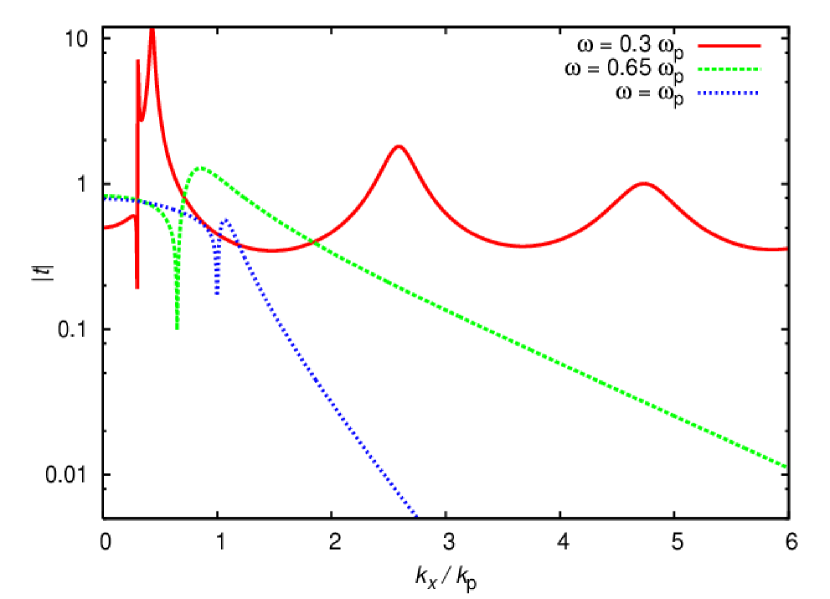
Figure 7: (Color online) The transmission coefficient, as defined in equation (9), with the surrounding medium taken to be air. The slab width used is $d=2/k_{\mathrm{p}}$, which would be of the order of 100nm for a plasma frequency $\omega_{\mathrm{p}}\sim 4$eV. The results for three different frequencies are plotted, corresponding to the three bands referred to in the discussion of figure 4. The real part of $\epsilon_{x}$ is negative when $\omega=0.3\omega_{\mathrm{p}}$, while that of $\epsilon_{z}$ is positive; the signs are reversed when $\omega=0.65\omega_{\mathrm{p}}$. At higher frequencies, both are positive. The permittivity of the metal is taken to be $\epsilon_{\mathrm{m}}=1.7+0.6i-\omega_{\mathrm{p}}^{2}/\omega^{2}$, while that of the dielectric is $\epsilon_{\mathrm{d}}=2.5$.

At high frequencies (here represented by $\omega=\omega_{\mathrm{p}}$), both components of the metamaterial permittivity are positive. In this regime, the transmission coefficient is close to unity for small wave vectors. It drops abruptly to zero at $k_{x}=k_{0}$, and rises equally sharply afterward, again approaching unity; finally, it decays exponentially for larger wave vectors. Very similar behavior is observed in the intermediate frequency range ($\omega=0.65\omega_{\mathrm{p}}$). This time, the maximum following the zero at $k_{x}=k_{0}$ is higher, and the rate of exponential decay for large $k_{x}$ is less rapid.

The most interesting frequency range is the lowest one ($\omega=0.3\omega_{\mathrm{p}}$). There is the usual zero in the transmission at $k_{x}=k_{0}$, followed by a very sharp peak. However, there is also significant transmission even for large wave vectors; the transmission coefficient has a series of peaks, decreasing in magnitude, and approximately periodic in $k_{x}$. The resonances correspond to localized states for the slab; they are in turn antisymmetric and symmetric. There is a difference between the first two resonances (just above $k_{x}=k_{0}$) and those for higher wave vectors. For the first two, the wave is non-propagating inside the slab (because $k_{z}$ is almost purely imaginary): the resonances therefore consist of coupled surface plasmons located on each surface of the slab. For the higher wave vectors, the wave is able to propagate within the slab (because $k_{z}$ is almost purely real), and the transmission peaks correspond to Fabry-Perot resonances – standing waves inside the slab. (Yu et al., 2005)

In fact, a similar set of peaks would be visible in the intermediate-frequency regime, were it not for absorption. The material parameters used to generate figure 7 include a realistic amount of absorption, and a glance at figures 2 and 3 shows that absorption is high in the region where $\Re(\epsilon_{z})$ becomes negative. The localized states are supported in both the low- and intermediate-frequency ranges, but are suppressed in the latter by high absorption.

V Imaging a line source

We have seen that the layered system allows enhanced transmission of high-spatial-frequency components at certain frequencies. This gives us hope that we may achieve sub-wavelength imaging using the slab As a test, we consider the image of the line source pictured in figure 8.

Figure 8: (Color online) Imaging a solenoidal line source.

In the absence of the metamaterial, the field generated by this source is

$${\mathbf{E}}({\mathbf{r}})=\int_{-\infty}^{\infty}\int_{-\infty}^{\infty}e^{ik_{x}x+ik_{y}y+ik_{z}^{\prime}z-i\omega t}\tilde{E}_{0}(k_{y})\left(\hat{\mathbf{x}}-\frac{k_{x}}{k_{z}^{\prime}}\hat{\mathbf{z}}\right)\;dk_{x}\;dk_{y},$$ (10)

where the current profile in the $y$-direction is as yet unspecified. As before, $k_{z}^{\prime}$ represents the $z$-component of the wave vector in the surrounding medium.

When we place the metamaterial next to the source, as shown in the figure, some radiation will be reflected from the slab and will generate additional currents. If we neglect these, we can estimate the $x$-component of the transmitted field as

$$E_{x}^{\mathrm{TM}}({\mathbf{r}})=\int_{-\infty}^{\infty}\int_{-\infty}^{\infty}e^{ik_{x}x+ik_{y}y+ik_{z}^{\prime}(z-d)-i\omega t}t\left(\sqrt{k_{x}^{2}+k_{y}^{2}},\omega\right)\cdot\frac{\tilde{E}_{0}(k_{y})k_{x}^{2}}{k_{x}^{2}+k_{y}^{2}}\;dk_{x}\;dk_{y}.$$ (11)

Note that this is the TM component of the field. In general, there will also be a TE component which must be calculated. However, if we consider a line source which is uniform in strength and infinitely long, so that $E_{0}(k_{y})\propto\delta(k_{y})$, the entire field is transverse magnetic. In this case, the calculation reduces to the solution of the following integral:

$$E_{x}^{\mathrm{TM}}({\mathbf{r}})=\frac{E_{0}}{k_{0}}\int_{-\infty}^{\infty}\frac{2e^{ik_{x}x+ik_{z}^{\prime}(z-d)-i\omega t}}{2\cos k_{z}d-i\left(\frac{k_{z}^{\prime}\epsilon_{x}}{k_{z}}+\frac{k_{z}}{k_{z}^{\prime}\epsilon_{x}}\right)\sin k_{z}d}\;dk_{x}.$$ (12)

The integral can be solved approximately when the frequency is in the intermediate range: that is, when $\Re(\epsilon_{x})>0$ and $\Re(\epsilon_{z})<0$. The resonant states then all have large $k_{x}$; they are the standing wave states discussed in the previous section, rather than the coupled surface plasmon states (which have $k_{x}$ close to $k_{0}$). We are therefore justified in making the near field approximation, which leads to the following analytic form for the $x$-component of the transmitted field:

$$E_{x}^{\mathrm{TM}}({\mathbf{r}})\approx\frac{\pm 4\pi iE_{0}}{k_{0}d\left(1/\epsilon_{z}-\epsilon_{x}\right)}\cdot\frac{e^{-ik_{1}\left(|x|-i(z-d)\right)-i\omega t}}{1+e^{-i\Delta k\left(|x|-i(z-d)\right)}},$$ (13)

where

$$k_{1}=\frac{1}{d}\sqrt{-\frac{\epsilon_{z}}{\epsilon_{x}}}\arctan\left(\frac{2\sqrt{-\epsilon_{x}\epsilon_{z}}}{1+\epsilon_{x}\epsilon_{z}}\right)$$ (14)

and

$$\Delta k=\frac{\pi}{d}\sqrt{-\frac{\epsilon_{z}}{\epsilon_{x}}}.$$ (15)

In this approximation, $E_{x}^{\mathrm{TM}}$ and $E_{z}^{\mathrm{TM}}$ are identical to within a phase factor. In figure 9, we plot the intensity of the transmitted field, comparing the approximate analytical solution with the results of numerical integration.

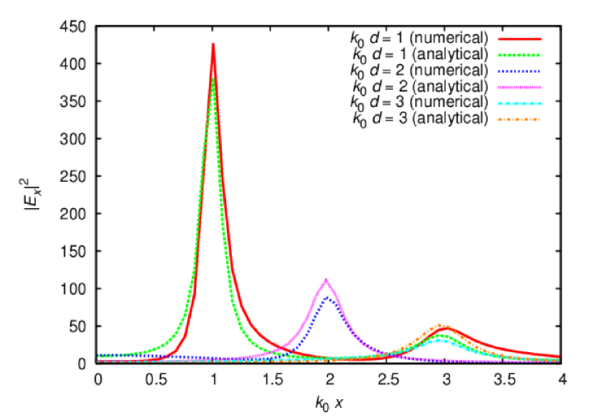
Figure 9: (Color online) The transmitted field intensity, comparing analytical and numerical results. The parameters used were $\epsilon_{\mathrm{d}}=2.5$, $\epsilon_{\mathrm{m}}=1.7+0.05i-\omega_{\mathrm{p}}/\omega^{2}$, with $\omega=0.68\omega_{\mathrm{p}}$. In each case, we plot the field just beyond the slab (so that for example when $k_{0}d=2.0$, $k_{0}z=2.01$).

To generate the plot, we take an unrealistically low value for the absorption in the metal; the point of the graph is to compare numerical and analytical results, but also to demonstrate the features which we hope to be able to observe.

First, we note that the position of the peaks is proportional to the slab width. This is a manifestation of the preferred direction of propagation; within the metamaterial, the light travels at a fixed angle to the $z$-axis, in the $xz$-plane (since we have translational invariance in the $y$-direction). The secondary peaks which are visible when $k_{0}d=1.0$ are caused by reflection from the boundaries; this is why they overlap precisely with the primary peaks for the slab with $k_{0}d=3.0$. The reflections are illustrated in figure 10.

Figure 10: (Color online) A schematic showing that reflections lead to periodically-repeated images of the two principal peaks.

In the first frequency regime, the approximate analytical solution is more difficult to obtain: there are the additional surface plasmon resonances close to $k_{x}=k_{0}$, for which one cannot make the near field approximation. However, it is still possible to obtain numerical results. As one would expect from figure 7, these are much more promising: using realistic parameters, we are able to produce a sharp image, as shown by the line marked “Effective medium” in figure 11.

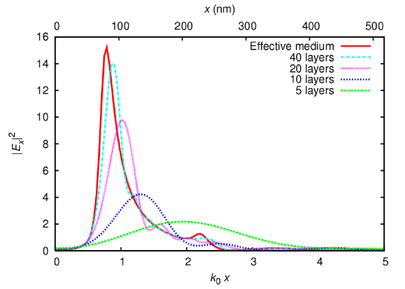
Figure 11: (Color online) The transmitted electric field intensity for a line source, imaged by a metamaterial slab of thickness $1/k_{0}$. The material parameters used correspond to layers of Ag and ZnS-SiO₂, embedded in crystalline Ge₂Sb₂Te₅ (a phase-change material used in optical storage devices), for light of wavelength 650nm. This corresponds to a total slab width of around 105nm.

The width of the principal peak in the effective medium approximation is around $\lambda/10$. Figure 11 also illustrates the results of a more detailed analysis, which goes beyond the simplified effective medium approach; we will discuss these next.

VI Beyond the effective medium approximation

Treating the layered system as an effective medium is a helpful simplification, in terms of both understanding and performing simulations. However, it has limitations. In this section, we model the system in more detail, considering the finite width of the layers; naturally, as the layers are made thinner, we see that the effective medium approximation becomes more appropriate.

First, we look at the dispersion relation for the layered metamaterial. We can obtain $k_{z}$ as a function of $k_{x}$ (at a given frequency) from the characteristic matrix, as described in appendix A. These isofrequency contours are plotted in figure 12.

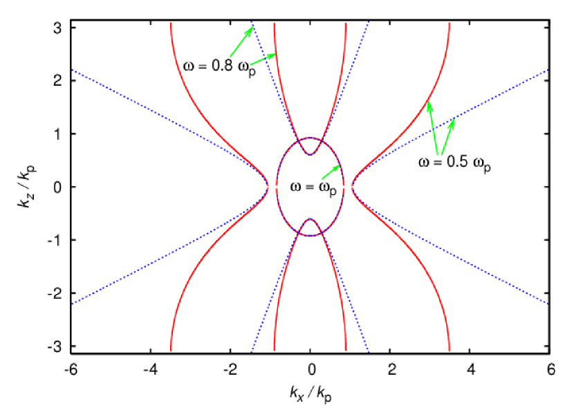
Figure 12: (Color online) Isofrequency contours demonstrating the effect of finite layer width. The solid lines are the contours for a system where the cell size ($d_{1}+d_{2}$) is $1/k_{\mathrm{p}}$; the result is a Brillouin zone of extent $2\pi$ on the $k_{z}$-axis. The dashed lines are the equivalent contours in the effective medium approximation. The three sets of contours correspond to the three bands of the dispersion relation discussed in section III; the first two are hyperbolic in the effective medium approximation, while the third is elliptical. The material parameters are the same as those used to generate figure 4.

The effective medium has full translational symmetry, but this is broken when considering the structure of finite-width layers; the system becomes periodic, and the figure shows part of the first Brillouin zone, which extends from $k_{z}=-\pi k_{\mathrm{p}}$ to $k_{z}=\pi k_{\mathrm{p}}$. The effective-medium contours are deformed by the new periodicity, and bend towards the zone boundaries. This introduces a new cutoff: for a given frequency, there is a value of $k_{x}$ above which no propagating solution exists. This affects the resolution of the lens-like system.

The next logical step is to investigate the change in the behavior of the slab of metamaterial described in section IV. From now on, we focus on the first band. Figure 13 shows that the new cutoff in $k_{x}$ is clearly manifested in the transmission function: above the cutoff, the transmission decays very rapidly.

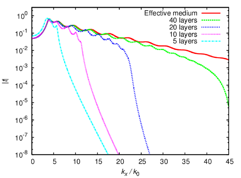
Figure 13: (Color online) The transmission as a function of $k_{x}$ for various layer widths. The total slab width is maintained at $1/k_{0}$ in each case, while the number of individual layers is adjusted.

Below the cutoff, we see the familiar Fabry-Perot and coupled surface plasmon resonances, although they have moved slightly; this is because the relationship between $k_{x}$ and $k_{z}$ has been altered, as shown in figure 12.

Finally, we re-examine the image of a line source using the modified transmission functions shown in figure 13. Figure 11 shows the transmitted electric field intensity, plotted as a function of $x$, for various different layer widths. Increasing the width of the layers which make up the metamaterial slab (while keeping the total slab width constant) causes the principal peak to broaden, as expected. As the layers get thinner, the transmitted image more closely resembles the effective medium result.

VII Conclusion

We have investigated a class of anisotropic materials in which the one of the components of the dielectric permittivity has a different sign from the others. These materials are able to support the propagation of modes that would normally be evanescent: they are able to collect and transfer the near field. In addition, inside the anisotropic medium, light travels in a preferred direction.

We have studied the transmission properties of a slab made up of such a material. The image of a line source consists of two lines, with an offset determined by the ratio of the components of the permittivity; the width of the imaged lines depends on the amount of absorption, but in principle can be much less than the wavelength of light used.

One realization of such a material is a stack of alternating layers of metal and dielectric. The thinner the layers, the better this metamaterial approaches the form of the ideal anisotropic medium. We have shown how the ideal band structure is deformed by the non-zero layer width. Using realistic material parameters, we have also demonstrated that a stack of alternating Ag and ZnS-SiO₂ layers can form an image of a line source which is much narrower than the wavelength of light when working at 650nm.

The combination of subwavelength resolution with the fact that the position of the image depends on the frequency of light being used suggests that this layered system may have useful applications. For example, in conjunction with a super-resolution near-field optical structure (super-RENS), (Liu et al., 2001; Lin et al., 2003) it may allow the possibility of multiplexed recording.

*

Appendix A Homogenization in layered systems

The effective medium parameters for our one-dimensional system of alternating layers can be calculated by using the characteristic matrix method. The effective dielectric permittivity is obtained from a consideration of TM fields; TE fields give the effective magnetic permeability.

The geometry of the system is shown in figure 1, with the $z$-axis perpendicular to the layers. We take the plane of incidence to be the $xz$-plane; the symmetry of the system means that this is equivalent to the $yz$-plane, and the results which follow are general.

The characteristic matrix ${\mathbf{M}}_{j}(k_{x},d)$ relates the Fourier component of the field in the plane $z=z_{0}$ to that in the plane $z=z_{0}+d$ (all within medium $j$). For TM waves in a homogeneous medium, it takes the form (Born and Wolf, 1980)

$${\mathbf{M}}_{j}(k_{x},d)=\begin{pmatrix}\cos k_{z}^{(j)}d&\frac{ik_{0}\epsilon_{j}}{k_{z}^{(j)}}\sin k_{z}^{(j)}d\\ \frac{ik_{z}^{(j)}}{k_{0}\epsilon_{j}}\sin k_{z}^{(j)}d&\cos k_{z}^{(j)}d\end{pmatrix}$$ (16)

where $k_{z}^{(j)}$ is given by the dispersion relation

$$k_{x}^{2}+(k_{z}^{(j)})^{2}=\epsilon k_{0}^{2}.$$ (17)

The matrix for a single cell of our layered system, consisting of one sheet of each material, is just the product of the matrices for the separate layers:

$${\mathbf{M}}_{\mathrm{cell}}(k_{x},d_{1},\eta)={\mathbf{M}}_{1}(k_{x},d_{1}){\mathbf{M}}_{2}(k_{x},\eta d_{1}).$$ (18)

A stack of $n$ cells has the characteristic matrix ${\mathbf{M}}_{n}=({\mathbf{M}}_{\mathrm{cell}})^{n}$. We can calculate this by diagonalizing ${\mathbf{M}}_{\mathrm{cell}}$; we then obtain

$${\mathbf{M}}_{n}=\frac{1}{p-q}\begin{pmatrix}-q\lambda^{n}+p\lambda^{-n}&\lambda^{n}-\lambda^{-n}\\ -pq(\lambda^{n}-\lambda^{-n})&p\lambda^{n}-q\lambda^{-n}\end{pmatrix}.$$ (19)

We have introduced $\lambda$, which is one of the eigenvalues of ${\mathbf{M}}_{\mathrm{cell}}$; the other eigenvalue is $\lambda^{-1}$, which follows because $\det{\mathbf{M}}_{\mathrm{cell}}=1$. We have also introduced $p$ and $q$, which are the ratios of the components of the eigenvectors of ${\mathbf{M}}_{\mathrm{cell}}$.

Expanding in powers of the layer thickness allows us to relate ${\mathbf{M}}_{n}$ to the characteristic matrix for an effective medium:

$${\mathbf{M}}_{n} =\begin{pmatrix}\cos k_{z}^{\mathrm{eff}}n(1+\eta)d_{1}&\frac{ik_{0}\epsilon_{x}}{k_{z}^{\mathrm{eff}}}\sin k_{z}^{\mathrm{eff}}n(1+\eta)d_{1}\\ \frac{ik_{z}^{\mathrm{eff}}}{k_{0}\epsilon_{x}}\sin k_{z}^{\mathrm{eff}}n(1+\eta)d_{1}&\cos k_{z}^{\mathrm{eff}}n(1+\eta)d_{1}\end{pmatrix}+\mathcal{O}\bigl{[}(1+\eta)d_{1}\bigr{]}$$ (20)

$$={\mathbf{M}}_{\mathrm{eff}}+\mathcal{O}\bigl{[}(1+\eta)d_{1}\bigr{]}$$ (21)

where the effective medium parameters are

$$\epsilon_{x} =\frac{\epsilon_{1}+\eta\epsilon_{2}}{1+\eta}$$ (22)

$$\frac{1}{\epsilon_{z}} =\frac{1}{\epsilon_{1}(1+\eta)}+\frac{\eta}{\epsilon_{2}(1+\eta)}.$$ (23)

These parameters appear in the dispersion relation for the effective medium, which differs slightly from (17) because the permittivity is now anisotropic:

$$\frac{k_{x}^{2}}{\epsilon_{z}}+\frac{(k_{z}^{\mathrm{eff}})^{2}}{\epsilon_{x}}=k_{0}^{2}.$$ (24)

We also note here that the cell matrix ${\mathbf{M}}_{\mathrm{cell}}$ has another use. We can determine the true dispersion relation for the layered system – without using the effective medium approximation – by finding the eigenvalues and eigenvectors of this matrix. When the eigenvalue has unit modulus, we have found a Bloch mode; we then make the association

$$\lambda=e^{ik_{z}(1+\eta)d_{1}}.$$ (25)

The eigenvalue $\lambda$ depends on the frequency and on $k_{x}$; equation (25) is therefore the dispersion relation.

References

- Ramakrishna et al. (2003) S. A. Ramakrishna, J. B. Pendry, M. C. K. Wiltshire, and W. J. Stewart, Journal of Modern Optics 50, 1419 (2003).
- Pendry (2000) J. B. Pendry, Physical Review Letters 85, 3966 (2000).
- Fang et al. (2005) N. Fang, H. Lee, C. Sun, and X. Zhang, Science 308, 534 (2005).
- Melville and Blaikie (2005) D. O. S. Melville and R. J. Blaikie, Optics Express 13, 2127 (2005).
- Ritchie (1957) R. H. Ritchie, Physical Review 106, 874 (1957).
- Cai et al. (2005) W. Cai, D. A. Genov, and V. M. Shalaev, Physical Review B 72, 193101 (2005).
- Ono et al. (2005) A. Ono, J. I. Kato, and S. Kawata, Physical Review Letters 95, 267407 (2005).
- Born and Wolf (1980) M. Born and E. Wolf, Principles of Optics (Pergamon Press, Oxford, 1980).
- Rytov (1955) S. M. Rytov, Journal of Experimental and Theoretical Physics 2, 466 (1955).
- Bergman (1978) D. Bergman, Physics Reports 43, 377 (1978).
- Yu et al. (2005) C. C. Yu, T. S. Kao, W. C. Lin, W. C. Liu, and D. P. Tsai, Journal of Scanning Microscopies 26, 90 (2005).
- Palik (1985) E. D. Palik, ed., Handbook of Optical Constants of Solids (Academic Press, London, 1985).
- Nikogosyan (1997) D. N. Nikogosyan, Properties of Optical and Laser-Related Materials (Wiley, Chichester, United Kingdom, 1997).
- Liu et al. (2001) W. C. Liu, C. Y. Wen, K. H. Chen, W. C. Lin, and D. P. Tsai, Applied Physics Letters 78, 685 (2001).
- Lin et al. (2003) W. C. Lin, T. S. Kao, H. H. Chang, Y. H. Lin, Y. H. Fu, C. Y. Wen, K. H. Chen, and D. P. Tsai, Japanese Journal of Applied Physics 42, 1029 (2003).