Test ion acceleration in the field of expanding planar electron cloud

Abstract

New exact results are obtained for relativistic acceleration of test positive ions in the laminar zone of a planar electron sheath evolving from an initially mono-energetic electron distribution. The electron dynamics is analyzed against the background of motionless foil ions. The limiting gamma-factor $\gamma_{p\infty}$ of accelerated ions is shown to be determined primarily by the values of the ion-electron charge-over-mass ratio $\mu=m_{e}Z_{p}/m_{p}$ and the initial gamma-factor $\gamma_{0}$ of the accelerated electrons. For $\mu>\frac{1}{8}$ a test ion always overtakes the electron front and attains $\gamma_{p\infty}>\gamma_{0}$. For $\mu<\frac{1}{8}$ a test ion can catch up with the electron front only when $\gamma_{0}$ is above a certain critical value $\gamma_{cr}$, which for $\mu\ll 1$ can most often be evaluated as $\gamma_{cr}=\frac{1}{4}\mu\exp\left(\mu^{-1}-1\right)$. In reality the protons and heavier test ions, for which $\gamma_{cr}>10^{398}$ is enormous, always lag behind the front edge of the electron sheath and have $\gamma_{p\infty}<\gamma_{0}$; for their maximum energy an appropriate intermediate asymptotic formula is derived. The domain of applicability of the laminar-zone results is analyzed in detail.

I Introduction

One of the most impressive latest achievements in laser-plasma interaction has been the observation of well-collimated high-energy proton and ion beams produced from thin metallic foils irradiated by ultra-intense sub-picosecond laser pulses ClKr.00 ; MaGu.00 ; SnKey.00 ; HeKa.02 . An exceptional quality, demonstrated recently for thus produced proton beams CoFu.04 , makes them very promising for many potential applications MoTa.06 .

In its gross features, the mechanism of ion acceleration in the cited and other similar experiments is believed to be reasonably well understood, and has been nicknamed TNSA (target normal sheath acceleration) HaBr.00 ; WiLa.01 . High directionality and low phase volume of generated protons CoFu.04 indicate that they are accelerated in a highly ordered electric field normal to the virtually unperturbed planar rear surface of the laser-irradiated foil. The electric field is caused by charge separation in the sheath layer that is formed by energetic electrons generated by absorption of the laser pulse.

However, an attempt to provide a more detailed and comprehensive theoretical description leads to a very complex system of plasma dynamics equations that can hardly be ever solved rigorously. To establish practically useful dependences and relations, one has to introduce additional simplifications. As is typical in other areas of physics, of particular value for gaining a deeper understanding of the process of ion acceleration prove to be certain particular idealized but exactly solvable problems. Salient and well known examples are (i) a self-similar evolution of the ion distribution function by quasi-neutral plasma expansion into vacuum GuPa.65 , and (ii) a virtually exact two-fluid solution of the isothermal plasma expansion with a full account of charge separation effects Mora03 . In this paper we present a rigorous solution and a full parametric analysis of another such idealized problem, namely, the problem of test ion acceleration in a dynamic sheath of relativistic electrons with the delta-function initial velocity distribution.

Typically, fast protons in laser irradiated metallic foils originate from a thin (few nanometers) contaminant layer of water and hydrocarbons at the foil surface GiJo.86 ; SnKey.00 ; HeKa.02 . Then, a natural simplification would be to assume that the heavy bulk ions (like Au for example) of a metallic foil are infinitely heavy and stay at rest, while the accelerated protons are treated as test positive charges initially located at the foil surface. Our present solution is essentially based on this assumption.

Next, one has to choose how to treat the electrons. A widely used assumption is that the electrons instantaneously relax to the equilibrium Boltzmann distribution in the time-dependent electrostatic potential of the expanding plasma: it was employed in both solutions GuPa.65 ; Mora03 cited above. With immobile ions, such an assumption allows straightforward calculation of the electrostatic sheath potential $\phi(x)$ either in the one-temperature CrAu.75 or multi-temperature PaTi.04 cases. An obvious problem with this approximation is that it leads to a diverging result for the maximum energy of accelerated test ions because the corresponding potential $\phi(x)=-(2T/e)\ln\left[1+x/(\sqrt{2}\lambda_{D})\right]$ CrAu.75 logarithmically diverges at $x\to+\infty$ in the planar geometry; here $\lambda_{D}$ is the Debye length at the base of the electron sheath with temperature $T$, $+e$ is the elementary charge. However, as was pointed out by Gurevich et al. GuPa.65 , this divergence is not physical because even if one assumes that the hot electrons have a perfect Maxwellian distribution initially, at $t=0$, it still takes an increasingly long time $\Delta t\simeq t_{eq}(x)\propto x$ for the Boltzmann relation $n_{e}\propto\exp(e\phi/T)$ to establish at an increasingly large distance $x$ from the initial plasma surface (for more details see section III.2.2 below). As possible remedies, attempts have been made to use ad hoc quasi-equilibrium electron distributions truncated either at high velocities PeMo78 ; KiMi.83 or at large distances PaLo04 . Evidently, neither of these two approaches is fully self-consistent.

Without the Boltzmann relation, a self-consistent treatment requires that one starts with a given initial electron distribution function at $t=0$, and then calculates its evolution for $t>0$. For high-energy (multi-MeV) electrons this can be done in the collisionless approximation. In this work we solve this problem in the simplest case of initially monoenergetic electrons, i.e. when at $t=0$ all the free electrons of a uniform planar foil have one and the same initial velocity $v_{0}$ perpendicular to the foil. Rigorous results are obtained for test ion acceleration in the outer laminar zone (for strict definition see section III.1 below) of the dynamically evolving electron sheath. Particular attention is paid to the limiting energy of accelerated ions at $t\to\infty$, which is always finite within the adopted model.

This paper is not the first publication addressing thus formulated problem: to a significant extent, it builds upon earlier work by Bulanov et al. BuEs.04 . The new progress made here includes the following key issues. Temporal behavior of the boundary between the outer laminar and the inner relaxation zones of the dynamically evolving electron sheath is studied in detail. Consequently, the domain of applicability of the laminar-zone results for test ions is clearly identified in the full parameter space of the problem. In contrast to Ref. BuEs.04 , the electric field in the laminar zone is calculated exactly and not to the accuracy of the linear in $x$ term. It is proven that the answer to the intriguing question of whether a test ion can overtake the electron front (and, consequently, surpass the initial electron velocity $v_{0}$) is determined by a critical relationship between the initial gamma-factor $\gamma_{0}$ of accelerated electrons and the ion-electron charge-over-mass ratio $\mu$ [defined in Eq. (1) below]. A fully relativistic intermediate asymptotic formula (58) is derived which may be used in realistic situations to evaluate the maximum energy of accelerated protons and heavier ions.

II Formulation of the problem

Consider a uniform electrically neutral plasma foil of thickness $l_{0}$ with an initial density of free electrons $n_{0}$. At time $t=0$ all the free electrons are set in motion with the same initial velocity $v_{0}$ perpendicular to the foil (see Fig. 1); $v_{0}$ can be arbitrarily close to the speed of light $c$. At later times $t>0$ the motion of electrons, treated as a collisionless charged fluid, is governed by the electric field $E(t,x)$, which arises due to charge separation in the evolving plasma cloud. The origin of the $x$-axis, directed along the initial electron velocity $\vec{v}_{0}$, is chosen at the forward foil surface, so that initially the foil occupies the region $-l_{0}\leq x\leq 0$. The bulk foil ions are assumed to be infinitely heavy and staying at rest. Our goal is to calculate the motion of a test ion of charge $+eZ_{p}$ and mass $m_{p}$ placed initially at the foil surface $x=0$, which is accelerated by the electric field $E(t,x)$ in the positive direction of the $x$ axis. Note that here and below $m_{p}$ is not necessarily the proton mass.

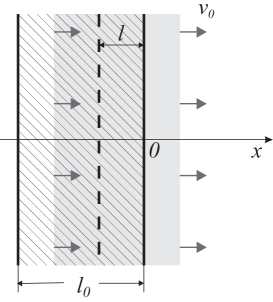
Figure 1: Schematic view of a plasma foil with motionless bulk ions (hatched area) and electrons (grey area) boosted to a velocity $v_{0}$. Dashed vertical line marks the initial position of electrons with the Lagrangian coordinate $l$.

It is easy to understand that this problem is governed by only three independent dimensionless parameters, which we choose to be

$$\mu=\frac{m_{e}Z_{p}}{m_{p}},\quad\Lambda=\frac{l_{0}\omega_{0}}{v_{0}\sqrt{\gamma_{0}}},\quad\gamma_{0}=(1-\beta_{0}^{2})^{-1/2};$$ (1)

here $m_{e}$ is the electron mass,

$$\omega_{0}=\left(\frac{4\pi e^{2}n_{0}}{m_{e}}\right)^{1/2}$$ (2)

is the plasma frequency in the initial configuration, $e$ is the positive elementary charge, and $\beta_{0}=v_{0}/c$. If a proton (or some other light ion) is chosen as a test particle, the charge-over-mass ratio $\mu$ is small, $\mu\leq 1/1836\ll 1$. We will, however, explore the entire possible range of $0<\mu<\infty$, firstly, for the sake of completeness of the analysis, and, secondly, keeping in mind that light positive particles — such as positrons, $\pi^{+}$ or $\mu^{+}$ mesons — may in principle be created and accelerated under an intense laser irradiation.

For a non-thermal electron cloud considered here the quantity $v_{0}\sqrt{\gamma_{0}}/\omega_{0}$ plays a role of the Debye length. Then, the parameter $\Lambda$ is the initial foil thickness in units of the Debye length. Of particular interest is the limit $\Lambda=0$ of a geometrically infinitely thin foil which, however, has a finite number

$$\Sigma=n_{0}l_{0}$$ (3)

of electrons per unit surface area. On the one hand, the effects of charge separation are the strongest in this limit for a given value of $v_{0}$. On the other hand, it is in this limit that most of the exact results can be established analytically; many of them are then straightforwardly extended to a more general case of $\Lambda\gtrsim 1$.

Parameter $\gamma_{0}$ is the relativistic gamma-factor of the accelerated electrons. In the non-relativistic limit of $\beta_{0}\ll 1$, when $\gamma_{0}\approx 1+\frac{1}{2}\beta_{0}^{2}$, this parameter becomes irrelevant, and we are left with only two principal parameters $\mu$ and $\Lambda$. On a par with $\beta_{0}$ and $\gamma_{0}$, the dimensionless momentum $\Pi_{0}=\beta_{0}\gamma_{0}$ is used below as the principal kinematic characteristic of the accelerated electrons.

III Motion of electrons

III.1 General notation and relationships

Motion of electrons is described by a function $x_{e}(t,l)$ [or by a function $x_{e}(t,\xi)$], where $l$ (or $\xi$) is a Lagrangian coordinate in the electron fluid: $x_{e}(t,l)$ is the position at time $t$ of an electron whose original position at $t=0$ was $x_{e}(0,l)=-l$ (the broken line in Fig. 1). The dimensionless Lagrangian coordinate $0\leq\xi\leq 1$ is defined as

$$\xi=\frac{l}{l_{0}}.$$ (4)

Then, the front edge of the electron cloud is at $\xi=0$, its rear edge is at $\xi=1$.

At any fixed time $t$ one can invert $x_{e}(t,\xi)$ with respect to $\xi$ to obtain the inverse function $\xi=\xi(t,x)$ defined inside the expanding electron cloud. Without electron-electron collisions the function $\xi(t,x)$ ceases to be single-valued with respect to $x$ after some time — even if it were so initially. In this paper we use the term “laminar zone” for that region of the electron cloud where $\xi(t,x)$ is single-valued (see Figs. 2 and 3 below). In the remaining “relaxation zone”, where $\xi(t,x)$ is multi-valued, electrons gradually relax to the equilibrium Boltzmann distribution.

The function $x_{e}(t,\xi)$ is found by solving the following equations of electron motion

$$\frac{1}{c}\frac{dx_{e}}{dt} = \frac{\Pi_{e}}{\sqrt{1+\Pi_{e}^{2}}}\equiv\beta_{e},$$ (5a)

$$\frac{d\Pi_{e}}{dt} = -\frac{e}{m_{e}c}\,E(t,x_{e}),$$ (5b)

where $\beta_{e}=v_{e}/c$, and $\Pi_{e}=\beta_{e}\gamma_{e}=\beta_{e}(1-\beta_{e}^{2})^{-1/2}$; the Lagrangian time derivative $d/dt$ is calculated at a fixed $\xi$. As is well known, equations (5) admit the energy integral

$$m_{e}c^{2}\Sigma\int\limits_{0}^{1}\gamma_{e}(t,\xi)\,d\xi+\frac{1}{8\pi}\int\limits_{-\infty}^{+\infty}E^{2}\,dx=m_{e}c^{2}\Sigma\,\gamma_{0}.$$ (6)

The electric field $E(t,x)$ is obtained by solving the Poisson equation, which in the planar geometry of our problem yields

$$E(t,x)=4\pi e\Sigma\left[\sigma_{e}(t,x)-\sigma_{i}(x)\right];$$ (7)

here $0\leq\sigma_{e}(t,x)\leq 1$ [$0\leq\sigma_{i}(x)\leq 1$] is the fraction of the total number of electrons (ions) above $x$ at time $t$, i.e.

$$\sigma_{e}(t,x)=\frac{1}{\Sigma}\int\limits_{x}^{\infty}n_{e}(t,x^{\prime})\,dx^{\prime}.$$ (8)

For motionless ions one obviously has

$$\sigma_{i}(x)=\left\{\begin{array}[]{ll}1,&x<-l_{0},\\ -x/l_{0},&-l_{0}\leq x\leq 0,\\ 0,&x>0.\end{array}\right.$$ (9)

Calculation of $\sigma_{e}(t,x)$ depends on whether $x$ happens to be in the laminar or relaxation zone of the electron cloud. In the laminar zone one simply has $\sigma_{e}(t,x)=\xi(t,x)$, and equations of motion (5) can be solved analytically.

In the relaxation zone, where the function $\xi(t,x)$ becomes multi-valued with respect to $x$, one has to use a more general expression

$$\sigma_{e}(t,x)=\sum_{x_{e}(t,\xi)>x}\Delta\xi,$$ (10)

where summation is done over all the segments $\Delta\xi$ which at time $t$ are located inside the interval $(x,+\infty)$. Clearly, if Eqs. (5) are to be solved with a full account of the relaxation zone, it can only be done numerically. To this end, a numerical code TIAC (test ion acceleration) has been written, which calculates the electron motion and the ensuing electric field $E(t,x)$ with a full account of possible mutual interpenetration of different elements of the electron fluid. Because of rapid randomization (for details see subsection III.2.2) of the electron motion at the core of the relaxation zone, such straightforward calculations can only be realized within a limited time span of the order of 100 periods of electron oscillations near the foil surface.

III.2 Solution for $\Lambda=0$

Here we consider the limit $l_{0}\to 0$ of a geometrically very thin foil with a finite value of electron number per unit area $\Sigma=n_{0}l_{0}$, where both the initial electron density $n_{0}$ and the plasma frequency $\omega_{0}$ become formally infinite. In this case it is convenient to introduce the following units of time and length

$$[t]=t_{\Sigma}\equiv\frac{m_{e}v_{0}}{4\pi e^{2}\Sigma}\,\gamma_{0},\quad[x]=l_{\Sigma}\equiv v_{0}t_{\Sigma},$$ (11)

which replace the usual time and length scales $\sqrt{\gamma_{0}}/\omega_{0}$, $v_{0}\sqrt{\gamma_{0}}/\omega_{0}$ in a finite-density plasma. Evidently, the length unit $l_{\Sigma}$ plays a role of the Debye length in our dynamic electron sheath. Below, the quantities measured in units (11) are marked with a bar. The electron trajectories are represented by a two-parameter family of curves $\bar{x}_{e}(\bar{t},\xi,\beta_{0})$.

III.2.1 Electron trajectories

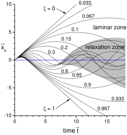
Figure 2: Electron trajectories for $\Lambda=0$ in the non-relativistic limit of $\Pi_{0}\ll 1$. Each curve is marked by the corresponding $\xi$ value. The relaxation zone is shown as a grey shaded area.

In the laminar zone, where $\sigma_{e}=\xi$, Eqs. (5) are solved analytically. The two relevant branches of this solution, obtained with the initial conditions $\bar{x}_{e}(0,\xi,\beta_{0})=0$, $\Pi_{e}(0,\xi,\beta_{0})=\Pi_{0}\equiv\beta_{0}\gamma_{0}$, are

$$\Pi_{e} = \Pi_{0}(1-\xi\bar{t}),$$ (12a)

$$\bar{x}_{e} = \frac{\bar{t}(2-\xi\bar{t})}{1+\sqrt{1-\beta_{0}^{2}\xi\bar{t}(2-\xi\bar{t})}},$$ (12b)

for $0<\bar{t}<2/\xi$, and

$$\Pi_{e} = \Pi_{0}\left[(1-\xi)\bar{t}+1-2/\xi\right],$$ (13a)

$$\bar{x}_{e} = \frac{\bar{t}^{2}(1-\xi)+2\bar{t}(1-2/\xi)+4/\xi^{2}}{1+\sqrt{1-\beta_{0}^{2}\xi\bar{t}(2-\xi\bar{t})}},$$ (13b)

for $2/\xi<\bar{t}<2/\left[\xi(1-\xi)\right]$.

In the upper half-space $\bar{x}_{e}>0$ Eq. (12b) is easily inverted with respect to $\xi$, which leads us to the following expression for the electric field

$$E(\bar{t},\bar{x})=4\pi e\Sigma\,\xi(\bar{t},\bar{x})=8\pi e\Sigma\,\frac{\bar{t}-\bar{x}}{\bar{t}^{2}-\beta_{0}^{2}\bar{x}^{2}}.$$ (14)

Inside the relaxation zone, where the electron trajectories intersect with one another, one has to abandon Eqs. (12)–(14) and solve Eqs. (5) numerically to calculate $\bar{x}_{e}(\bar{t},\xi,\beta_{0})$ and $E(\bar{t},\bar{x})$.

In the non-relativistic limit $\bar{x}_{e}(\bar{t},\xi)=\bar{x}_{e}(\bar{t},\xi,0)$ is a universal function of two variables $\bar{t}$ and $\xi$. It is plotted in Fig. 2 for a selection of $\xi$ values as calculated with the TIAC code. In Fig. 3 the non-relativistic function $\bar{x}_{e}(\bar{t},\xi)$ is plotted versus $\xi$ for $\bar{t}=20$. Qualitatively, the relativistic trajectories $\bar{x}_{e}(\bar{t},\xi,\beta_{0})$ look similar to $\bar{x}_{e}(\bar{t},\xi,0)$. In particular, for any $0<\beta_{0}<1$ the rear edge of the electron cloud $\xi=1$ turns around (i.e. has $\Pi_{e}=0$) at $\bar{t}=1$, and later crosses the foil at $\bar{t}=2$ with $\Pi_{e}=-1$. During the period $0<\bar{t}<2$ there exists a vacuum gap between the foil ions and the ejected electrons. After its closure, the front and the rear edges of the electron cloud propagate freely in opposite directions with constant velocities $\pm v_{0}$.

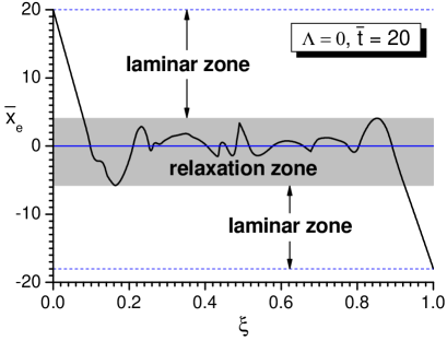
Figure 3: Position of individual electrons $\bar{x}_{e}(\bar{t},\xi)$ in the non-relativistic case at time $\bar{t}=20$. Without electron-electron collisions, $\bar{x}_{e}(\bar{t},\xi)$ is non-monotonic with respect to the Lagrangian coordinate $\xi$ in the relaxation zone (shaded area). The number of local minima and maxima along $\xi$ rapidly (exponentially) increases with time.

Numerical solution of Eqs. (5) enables one to trace the onset and subsequent expansion of the relaxation zone, shown in Figs. 2 and 3 as shaded areas. In this zone oscillations of electrons around the positively charged foil, occurring on a time scale $t_{\Sigma}$, rapidly become stochastic and ultimately lead to establishment of the Maxwell-Boltzmann distribution with a certain temperature that can be found from the energy integral (6). The starting point of the relaxation zone can be calculated analytically by applying the conditions $\partial\bar{x}_{e}/\partial\xi=0$, $\partial^{2}\bar{x}_{e}/\partial\xi^{2}=0$ to Eq. (13b); in the non-relativistic limit it has the coordinates

$$\bar{t}_{r0}=\frac{27}{4},\quad\xi_{r0}=\frac{4}{9},\quad\bar{x}_{r0}=-\frac{27}{32},$$ (15)

which become

$$\bar{t}_{r0}=6,\quad\xi_{r0}=\frac{1}{2},\quad\bar{x}_{r0}=-2.$$ (16)

in the ultra-relativistic limit $\gamma_{0}\gg 1$.

III.2.2 Evolution of the relaxation zone

Even though electrons are treated as a collisionless fluid, the presence of a positively charged ion sheet is sufficient for the electron subsystem to develop a stochastical behavior. Once the electron trajectories in the central region begin to intersect one another in the process of oscillations across the ion layer (see Fig. 2), their further motion becomes increasingly stochastic. As a result, an isothermal quasi-equilibrium core gradually develops inside the relaxation zone, where the electron density obeys the Boltzmann relation $n_{e}(x)\propto\exp\left(e\phi/T\right)$; here $\phi(x)$ is the equilibrium electrostatic potential, and $T$ is the temperature of the quasi-equilibrium core. This qualitative picture is fully confirmed by the results of direct simulations with the TIAC code presented in Fig. 4.

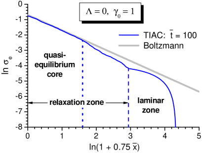
Figure 4: Spatial profile of the electron column density $\sigma_{e}(\bar{t},\bar{x})$ as calculated numerically with the TIAC code in the non-relativistic limit for $\bar{t}=100$. The equilibrium profile (20) obtained by using the Boltzmann relation is shown as a thick grey straight line.

Having adopted the Boltzmann relation, one easily solves the Poisson equation and obtains

$$\bar{\phi}(\bar{x})=-2\bar{T}\,\ln\left(1+\frac{|\bar{x}|}{4\bar{T}}\right),$$ (17)

where $\bar{\phi}$ and $\bar{T}$ are, respectively, the potential in units $m_{e}v_{0}^{2}\gamma_{0}/e$ and the temperature in units $m_{e}v_{0}^{2}\gamma_{0}$. The temperature $\bar{T}$ is found from the energy integral (6), which in our case transforms to a transcendental equation

$$2\bar{T}\beta_{0}^{2}+\frac{K_{0}\left(1/\beta_{0}\Pi_{0}\bar{T}\right)}{\gamma_{0}\,K_{1}\left(1/\beta_{0}\Pi_{0}\bar{T}\right)}=1;$$ (18)

here $K_{0}(z)$ and $K_{1}(z)$ are the modified Bessel functions. The limiting values of $\bar{T}$ are

$$\bar{T}=\left\{\begin{array}[]{ll}\displaystyle\frac{1}{3},&\Pi_{0}\ll 1,\\ \displaystyle\frac{1}{2},&\Pi_{0}\gg 1.\end{array}\right.$$ (19)

Figure 4 compares the equilibrium electron column density [as defined by Eq. (8)]

$$\left.\sigma_{e,eq}(\bar{x})\right|_{\bar{x}>0}=\frac{1}{2}\left(1+\frac{\bar{x}}{4\bar{T}}\right)^{-1},$$ (20)

calculated from Eq. (17), with that obtained from the TIAC numerical simulations in the non-relativistic limit for $\bar{t}=100$. One clearly distinguishes a quasi-equilibrium core of the relaxation zone, which is adequately described by the Boltzmann relation. Departures from the equilibrium are significant in the outer part of the relaxation zone and, of course, in the laminar zone.

To assess practical applicability of our results for test ion acceleration in the laminar zone, obtained below, one needs to know how the boundary $x_{r}(t)$ between the relaxation and the laminar zones evolves in time. We analyze this evolution by combining an analytical estimate in the limit of $t\to\infty$ with the TIAC simulations for times $\bar{t}\lesssim 100$.

Since randomization of the electron motion in the relaxation zone leads to establishment of the Maxwell-Boltzmann distribution, we can invoke the following argument to evaluate the width $\bar{x}_{r}$ of this zone at times $\bar{t}\gg 1$: by a time $\bar{t}$ the relaxation zone spreads to a distance $\bar{x}_{r}$ such that $\bar{t}=N_{r}\,\bar{t}_{eq}(\bar{x}_{r})$, where $N_{r}$ is a numerical factor of the order unity, and $\bar{t}_{eq}(\bar{x}_{r})$ is the travel time between $\bar{x}=0$ and $\bar{x}=\bar{x}_{r}$ in the equilibrium potential (17) of an electron whose kinetic energy vanishes at $\bar{x}=\bar{x}_{r}$. In a sense, $t_{eq}(x_{r})$ is a timescale on which the information about maxwellization of the velocity distribution up to a certain limiting value $v_{r}$ is transferred from $x=0$ to the corresponding limiting distance $x_{r}$ in the infinite potential well (17). This argument sounds perfectly reasonable for the quasi-equilibrium core, and may be surmised to apply to the entire relaxation zone as well.

The time $\bar{t}_{eq}(\bar{x}_{r})$ is given by an integral

$$\bar{t}_{eq}(\bar{x}_{r})=\int\limits_{0}^{\bar{x}_{r}}\frac{d\bar{x}}{\bar{v}_{e}(\bar{x})},$$ (21)

where the velocity $\bar{v}_{e}(\bar{x})$ is found from the energy integral

$$\gamma_{e}(\bar{x})-1=2\beta_{0}\Pi_{0}\bar{T}\,\ln\frac{4\bar{T}+\bar{x}_{r}}{4\bar{T}+\bar{x}}$$ (22)

for an electron moving in the static potential (17). After some algebra we obtain

$$\bar{t}_{eq}(\bar{x}_{r})=\frac{4\bar{T}+\bar{x}_{r}}{\sqrt{\gamma_{0}\bar{T}}}\int\limits_{0}^{\sqrt{\ln(1+\bar{x}_{r}/4\bar{T})}}\frac{1+2\beta_{0}\Pi_{0}\bar{T}z^{2}}{\sqrt{1+\beta_{0}\Pi_{0}\bar{T}z^{2}}}\,e^{-z^{2}}\,dz.$$ (23)

In the asymptotic limit of $\bar{x}_{r}\gg 1$ Eq. (23) yields $\bar{t}_{eq}(\bar{x}_{r})=\alpha_{eq}\bar{x}_{r}$, where the numerical coefficient $\alpha_{eq}$ is a weak function of $\Pi_{0}$: $\alpha_{eq}=\frac{1}{2}\sqrt{3\pi}$ for $\Pi_{0}\ll 1$, and $\alpha_{eq}=1$ for $\Pi_{0}\gg 1$. This leads us to a conclusion that asymptotically the ratio $\bar{x}_{r}(\bar{t})/\bar{t}$ should approach a certain constant value $\alpha_{r}$ (or oscillate in a narrow range around this value), which is fully confirmed by the TIAC simulations for times $\bar{t}\leq 100$.

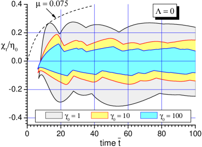
Figure 5: Evolution of the relaxation zone (shaded areas) for $\Lambda=0$ and three different values of $\gamma_{0}$ in terms of the hyperbolic variable $\chi_{r}$ [see Eq. (24)] normalized to $\eta_{0}=\textrm{arccosh}\gamma_{0}$ as calculated numerically with the TIAC code. The upper and the lower branches of the $\chi_{r}(\bar{t})$ curves correspond, respectively, to the boundaries in the upper ($x>0$) and lower ($x<0$) half-spaces. Dashed curve shows the test ion trajectory for $\gamma_{0}=1$ and $\mu=0.075$.

Figure 5 shows the temporal dependence of the upper and lower boundaries of the relaxation zone in terms of a hyperbolic variable $\chi_{r}=\chi_{r}(\bar{t})$ introduced via a relationship

$$\tanh\chi_{r}=\frac{x_{r}(t)}{ct}=\beta_{0}\frac{\bar{x}_{r}(\bar{t})}{\bar{t}}.$$ (24)

The fraction of the electron cloud occupied by the upper laminar zone is given by the difference $1-\chi_{r}/\eta_{0}$ [in the ultra-relativistic case the separation along the hyperbolic variable $\chi=\textrm{arctanh}(x/ct)$ is physically more representative than the separation along $x$], where $\eta_{0}=\textrm{arccosh}\,\gamma_{0}=\textrm{arcsinh}\,\Pi_{0}$. If $\chi_{r}(\bar{t})$ should reach the value $\eta_{0}$, it would mean that the relaxation zone has reached the electron front $\bar{x}=\bar{t}$ and the laminar zone has vanished. One clearly sees that typically the electron cloud is not dominated by the relaxation zone, whose fraction asymptotically approaches some constant value, and which has a tendency to shrink with the increasing $\gamma_{0}$. For $\gamma_{0}=1$ this fraction is $\alpha_{r}=0.25\pm 0.02$. Therefore, it can be expected that there exists a sizable window in the parameter space where the test ion acceleration takes place either entirely or predominantly in the laminar zone.

III.3 Solution for $\Lambda>0$

For a finite-thickness foil it is convenient to introduce a different pair of time and length units,

$$[t]=\Lambda t_{\Sigma}=\omega_{0}^{-1}\sqrt{\gamma_{0}},\quad[x]=\Lambda l_{\Sigma}=v_{0}\omega_{0}^{-1}\sqrt{\gamma_{0}},$$ (25)

where the time unit $[t]$ is based on the relativistic plasma frequency $\omega_{0}\gamma_{0}^{-1/2}$. In these units the frequency and the amplitude of the electron plasma oscillations are of the order unity for any value of $\gamma_{0}\geq 1$. Below, the quantities measured in units (25) are marked with a tilde. Note that in these units the dimensionless thickness of the foil is $\tilde{l}_{0}\equiv\Lambda$.

III.3.1 Electron trajectories

For subsequent analysis of the test ion motion we need the electron trajectories in the upper half-space $x>0$. However, because for $\Lambda>0$ each such trajectory $\tilde{x}_{e}(\tilde{t},\tilde{l})$ starts inside the foil at $-\Lambda\leq\tilde{x}\leq 0$, we should solve Eqs. (5) in this region as well, with the initial conditions $\tilde{x}_{e}(0,\tilde{l})=-\tilde{l}$, $\Pi_{e}(0,\tilde{l})=\Pi_{0}$. The required relativistic solution in the laminar zone at $-\Lambda\leq\tilde{x}_{e}\leq 0$ has the form

$$\tilde{x}_{e}(\tilde{t},\tilde{l},\beta_{0})=-\tilde{l}+h(\tilde{t},\beta_{0}),$$ (26)

where $h(\tilde{t},\beta_{0})$ is a periodic function of time $\tilde{t}$; for the first quarter-period it is implicitly given by the quadrature

$$\tilde{t}=\int\limits_{0}^{h}\frac{1-\frac{1}{2}\beta_{0}^{2}\zeta^{2}}{\sqrt{1-\zeta^{2}+\frac{1}{4}\beta_{0}^{2}\zeta^{4}}}\,d\zeta$$ (27)

Actually, this is a solution for a relativistic particle moving in a quadratic oscillator potential, for which one has the following energy integral

$$\sqrt{1+\Pi_{e}^{2}}+\frac{1}{2}\beta_{0}\Pi_{0}\,h^{2}=\gamma_{0}.$$ (28)

From Eq. (28) one readily establishes that the full amplitude (in units of $v_{0}\omega_{0}^{-1}\sqrt{\gamma_{0}}$) of plasma oscillations inside the foil is $2h_{0}$, where

$$h_{0}=\left(\frac{2\gamma_{0}}{\gamma_{0}+1}\right)^{1/2}.$$ (29)

In the non-relativistic limit, obtained by putting $\beta_{0}=0$ in Eq. (27), we have $h(\tilde{t})=\sin\tilde{t}$ and $h_{0}=1$.

Now, the trajectory of an electron $\tilde{l}$ in the laminar zone at $x>0$, which matches the solution (26), (27) at a point $\tilde{t}=\tilde{t}_{e1}$, $\tilde{x}_{e}=0$, can be written as

$$\tilde{x}_{e}(\tilde{t},\tilde{l},\beta_{0}) = \frac{R}{P+\sqrt{P^{2}-\beta_{0}^{2}\tilde{l}\,R}},$$ (30)

$$\Pi_{e}(\tilde{t},\tilde{l},\beta_{0}) = \Pi_{0}\left[Q-\tilde{l}\,(\tilde{t}-\tilde{t}_{e1})\right],$$ (31)

$$P=P(\tilde{l},\beta_{0}) = 1-\frac{1}{2}\,\beta_{0}^{2}\,\tilde{l}^{2},$$ (32)

$$Q=Q(\tilde{l},\beta_{0}) = \sqrt{1-\tilde{l}^{2}+\frac{1}{4}\,\beta_{0}^{2}\,\tilde{l}^{4}},$$ (33)

$$R=R(\tilde{t},\tilde{l},\beta_{0}) = (\tilde{t}-\tilde{t}_{e1})\left[2Q-\tilde{l}\,(\tilde{t}-\tilde{t}_{e1})\right],$$ (34)

$$\tilde{t}_{e1}=\tilde{t}_{e1}(\tilde{l},\beta_{0}) = \int\limits_{0}^{\tilde{l}}\frac{1-\frac{1}{2}\beta_{0}^{2}\zeta^{2}}{\sqrt{1-\zeta^{2}+\frac{1}{4}\beta_{0}^{2}\zeta^{4}}}\,d\zeta;$$ (35)

here the values of $\tilde{l}$ are confined to the interval $0\leq\tilde{l}\leq\min\{\Lambda,h_{0}\}$. The non-relativistic limit of this solution is easily recovered by putting $\beta_{0}=0$. To obtain the electric field in the laminar zone

$$E(\tilde{t},\tilde{x})=4\pi en_{0}v_{0}\omega_{0}^{-1}\gamma_{0}^{1/2}\;\tilde{l}(\tilde{t},\tilde{x}),$$ (36)

one needs the function $\tilde{l}(\tilde{t},\tilde{x},\beta_{0})$, which is the inverse of $\tilde{x}_{e}(\tilde{t},\tilde{l},\beta_{0})$ with respect to $\tilde{l}$. When calculating the results discussed in section IV.2, such inversion of Eqs. (30)-(35) was performed numerically.

Since the Lagrangian coordinate $\tilde{l}$ belongs to the interval $0\leq\tilde{l}\leq\Lambda$, a vacuum gap is formed between the ejected electrons and the ion layer in the case of $\Lambda<h_{0}$ for a limited time after the rear electron edge $\tilde{l}=\Lambda$ reaches the foil surface at $x=0$ — similar to the case of $\Lambda=0$ (see Fig. 2) where such a gap exists at $0<\bar{t}<2$. Throughout the gap, the electric field $E$ is constant and $\tilde{l}=\Lambda$. To avoid unnecessary technical complications, we exclude the interval $0<\Lambda<h_{0}<\sqrt{2}$ from our consideration, i.e. we perform all the calculations either for the limiting case of $\Lambda=0$, or for $\Lambda>h_{0}$ when no gap appears between the ejected electrons and the foil ions. The reward is that we get rid of the dependence of $\tilde{l}$ on the parameter $\Lambda$, i.e. $\tilde{l}(\tilde{t},\tilde{x},\beta_{0})$ is a smooth function of $\tilde{t}$ and $\tilde{x}$ for all $\tilde{t}\geq 0$ and $0\leq\tilde{x}\leq\tilde{t}$, and this function does not depend on $\Lambda$. In particular, this leads us to an important conclusion that the behavior of the electron trajectories (hence, the distribution of any other physical quantity) in the laminar zone of the electron cloud at $\tilde{x}>0$ does not depend on the parameter $\Lambda$ for $\Lambda>h_{0}$.

III.3.2 Evolution of the relaxation zone

The general arguments on the evolution of the relaxation zone formulated in section III.2.2 for $\Lambda=0$ remain valid at $\Lambda>0$ as well. In particular, these arguments lead us to the following estimate for the relative width of the relaxation zone

$$\left|\frac{\chi_{r}(t)}{\eta_{0}}\right|\leq\alpha_{\chi r}<\infty,$$ (37)

where $\chi_{r}(t)$ is defined in Eq. (24), and $\alpha_{\chi r}$ does not depend on time $t$ but is a function of $\Lambda$ and $\gamma_{0}$. Unfortunately, we have no rigorous proof that one can introduce an upper bound (37) valid at all times $t<\infty$. We have only been able to verify it numerically with the TIAC code within a limited range of $\Lambda\lesssim 20$, $\tilde{t}\lesssim 100$. As an example, Fig. 6 shows the evolution of the relaxation zone for $\Lambda=10$ and $\gamma_{0}=1$, 10, and 100.

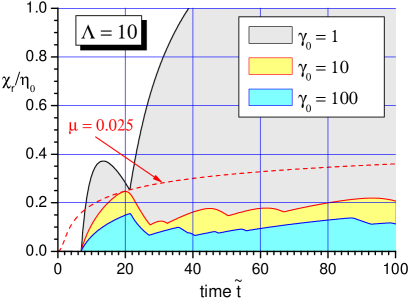
Figure 6: Same as Fig. 5 but for a finite foil thickness $\Lambda=10$. Shown here is the relaxation zone in the upper half-space $x>0$ above the initial foil surface $x=0$. Dashed curve is the test ion trajectory for $\gamma_{0}=10$ and $\mu=0.025$.

The TIAC simulations clearly indicate that the relative width of the relaxation zone $\alpha_{\chi r}$ increases with the increasing $\Lambda$, and decreases with the increasing $\gamma_{0}$. In particular, in the non-relativistic limit of $\gamma_{0}\to 1$ we have $\alpha_{\chi r}>1$ for $\Lambda>5.45$, i.e. for $\Lambda>5.45$ the laminar zone completely vanishes after some time (see Fig. 6). However, it reappears already at moderately relativistic electron energies $\gamma_{0}\gtrsim 4$, and becomes quite broad at $\gamma_{0}>10$–100, when we have $\alpha_{\chi r}\lesssim 0.2$–0.3. The latter implies that the laminar-zone regime of test ion acceleration should be particularly relevant to highly relativistic electron clouds with $\gamma_{0}\gtrsim 100$.

In the previous subsection it was established that the electron trajectories in the laminar zone do not depend on $\Lambda$ for $\Lambda>h_{0}$. This, however, does not mean that the same should apply to the boundary between the relaxation and the laminar zones because this boundary is determined by electrons traversing the relaxation zone. Nevertheless, one might expect that the curve $\chi_{r}(\tilde{t})$ should approach a certain limiting form for a fixed $\gamma_{0}$ and $\Lambda\to\infty$: such a limit would correspond to the case where the bulk plasma ions occupy the entire half-space $x<0$. However, the existence of such limit for all $t<\infty$ is far from obvious. Numerical simulations show that only the initial portion of the $\chi_{r}(\tilde{t})$ curve around its first local maximum at $\tilde{t}\simeq 15$–20 (see Figs. 5 and 6) becomes independent of $\Lambda$ for $\Lambda\gtrsim 2.5$.

IV Motion of test ions

Acceleration of a positive test ion with a charge $+eZ_{p}$ and a mass $m_{p}$ (in conventional units) is described by the following equations of motion

$$\frac{1}{c}\frac{dx_{p}}{dt} = \frac{\Pi_{p}}{\sqrt{1+\Pi_{p}^{2}}}\equiv\beta_{p},$$ (38a)

$$\frac{d\Pi_{p}}{dt} = +\frac{eZ_{p}}{m_{p}c}\,E(t,x_{p}),$$ (38b)

where $x_{p}(t)$ is the position of the ion, and $\Pi_{p}(t)=\beta_{p}\gamma_{p}=\beta_{p}(1-\beta_{p}^{2})^{-1/2}$ is its momentum in units of $m_{p}c$. As a rule, we assume that the test ion starts at $t=t_{p0}=0$ with the initial values $x_{p}(t_{p0})=\Pi_{p}(t_{p0})=0$. Then, because the electric field $E(t,x)$ is non-negative for all $x\geq 0$, we are guaranteed that $x_{p}(t)>0$ for all $t>0$. Equations (38) bring in a dimensionless parameter $\mu=m_{e}Z_{p}/m_{p}$, which contains all the necessary information about the test ion.

IV.1 Solution for $\Lambda=0$

Here, as in section III.2, we use the units (11) and mark thus normalized quantities with a bar. The accelerating electric field $E(\bar{t},\bar{x})$ in the laminar zone is given by Eq. (14).

IV.1.1 Vacuum phase

When $\Lambda=0$, a test ion begins its motion by passing through a vacuum gap, where it is accelerated by a constant field $E=4\pi e\Sigma$, until its trajectory

$$\bar{x}_{p,vac}(\bar{t})=\frac{1}{\mu\beta_{0}\Pi_{0}}\left(\sqrt{1+\mu^{2}\Pi_{0}^{2}\bar{t}^{2}}-1\right)$$ (39)

crosses the rear edge [$\xi=1$ in Eq. (12b)] of the electron cloud at

$$\bar{t}=\bar{t}_{p1}=\frac{2(1+\mu\gamma_{0})}{1+2\mu\gamma_{0}+\mu^{2}},\quad\bar{x}=\bar{x}_{p1}=\bar{x}_{p,vac}(\bar{t}_{p1})$$ (40)

with a momentum $\Pi_{p1}=\mu\Pi_{0}\bar{t}_{p1}$. The latter values should be used as the initial conditions for further acceleration inside the electron cloud.

IV.1.2 Non-relativistic solution

In the non-relativistic limit a general analytical solution is easily found to Eqs. (38). The type of this solution depends on whether the roots $\lambda$ and $1-\lambda$ of the characteristic equation

$$\lambda^{2}-\lambda+2\mu=0$$ (41)

are real or complex. In this way a critical value $\mu_{\ast}=\frac{1}{8}$ of the parameter $\mu$ is established, which separates the two solution types. For $\mu>\frac{1}{8}$, when $\lambda$ is complex, a test ion always catches up with the electron front $\bar{x}=\bar{t}$ and acquires the final velocity $v_{p\infty}$ in excess of the initial electron velocity $v_{0}$.

In the physically more interesting case of $\mu<\frac{1}{8}$ (a sufficiently heavy test ion) the sought for solution of Eqs. (38) is given by

$$\bar{x}_{p}(\bar{t})=\bar{t}-C_{1}\bar{t}^{1-\lambda}+C_{2}\bar{t}^{\lambda},$$ (42)

where

$$\lambda=\frac{1}{2}\left(1-\sqrt{1-8\mu}\right)$$ (43)

is the smaller of the two real roots of Eq. (41), and the integration constants

$$C_{1}=\frac{2^{\lambda}(1-\lambda-\mu)}{(1-2\lambda)(1+\mu)^{1+\lambda}},\quad C_{2}=\frac{2^{1-\lambda}(\lambda-\mu)}{(1-2\lambda)(1+\mu)^{2-\lambda}}$$ (44)

are calculated by using the initial conditions (40) for $\gamma_{0}=1$; Eq. (42) applies at $\bar{t}\geq\bar{t}_{p1}=2/(1+\mu)$.

Solution (42) reveals the following general features of ion acceleration in the laminar zone. The distance $\bar{t}-\bar{x}_{p}(\bar{t})$ between the electron front and the accelerated ion increases monotonically with time, i.e. a test ion with $\mu<\frac{1}{8}$ lags further and further behind the electron front as $t\to\infty$. At the same time, the ion velocity $v_{p}(t)=dx_{p}/dt$ monotonically grows in time, and in the formal limit of $t\to\infty$ it asymptotically approaches the initial electron velocity $v_{0}$ — as it has been established earlier in Ref. BuEs.04 . The latter, however, occurs on an extremely long timescale $\bar{t}_{ac}\simeq\exp\left(\frac{1}{2}\mu^{-1}\right)$, which is beyond any realistic value for protons and other ions with $\mu\leq 1/1836$. From practical point of view, an intermediate asymptotics

$$v_{p}(t)\approx 2\mu v_{0}\,\ln\left(\frac{2\pi e^{2}\Sigma}{m_{e}v_{0}}\,t\right),$$ (45)

inferred from Eqs. (42)–(44) for $\mu\ll 1$ and $1\ll\bar{t}\ll\exp\left(\frac{1}{2}\mu^{-1}\right)$, might be of interest — if not the presence of the relaxation zone. The fact is that solution (42) applies only for ions with $0.0745\leq\mu<0.125$ because, as one finds from the TIAC simulations (see Fig. 5), the ion trajectories for $\Lambda=0$ and $\mu<0.0745$ penetrate into the relaxation zone. Ions with $\mu\leq 1/1836$ are accelerated deep in the relaxation zone, where one can use the Boltzmann relation and the quasi-static potential (17); one readily verifies that the potential (17) leads to much higher (by roughly a factor $\mu^{-1}$) final ion energies than those obtained from Eq. (45). From this we conclude that the acceleration in the near-front laminar zone of a non-relativistic electron cloud is never important for protons and heavier test ions. In section IV.2 we demonstrate that this conclusion, proved here for $\Lambda=0$, is valid for $\Lambda>1$ as well.

IV.1.3 Relativistic solution

Analysis of ion motion in the general relativistic case is significantly simplified after we make a transformation from the dynamic variables $x_{p}$ and $\Pi_{p}$ to hyperbolic variables $\chi$ and $\eta$ defined by means of the relationships

$$\tanh\chi=\frac{x_{p}}{ct}=\beta_{0}\frac{\bar{x}_{p}}{\bar{t}},\quad\sinh\eta=\Pi_{p}.$$ (46)

Accordingly, the initial electron velocity $v_{0}$ is represented by a parameter $\eta_{0}$, where $\Pi_{0}=\sinh\eta_{0}$, $\gamma_{0}=\cosh\eta_{0}$, $\beta_{0}=\tanh\eta_{0}$. In terms of these variables equations (38) with the expression (14) for the electric field become

$$\frac{d\chi}{d\zeta} = \frac{\cosh\chi}{\cosh\eta}\,\sinh(\eta-\chi)$$ (47a)

$$\frac{d\eta}{d\zeta} = 2\mu\,\frac{\cosh\chi}{\cosh\eta}\,\sinh(\eta_{0}-\chi),$$ (47b)

where $\zeta=\ln\bar{t}$. Equations (47) do not contain the independent variable $\zeta$ on their right-hand sides, which means that certain key features of the ion motion can be analyzed by inspecting the integral curves of the first-order phase equation

$$\frac{d\eta}{d\chi}=2\mu\,\frac{\sinh(\eta_{0}-\chi)}{\sinh(\eta-\chi)}$$ (48)

in the ($\chi,\eta$) plane. Of principal importance here is the singular point $(\chi,\eta)=(\eta_{0},\eta_{0})$.

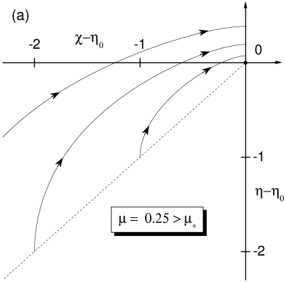
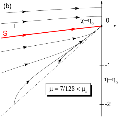
Figure 7: Phase trajectories for the ion equations of motion in the form (47) in the vicinity of the singular point $(\chi,\eta)=(\eta_{0},\eta_{0})$ for two values of parameter $\mu$. The singular point is a focus for $\mu>\mu_{\ast}=\frac{1}{8}$ (a), and a node for $\mu<\mu_{\ast}$ (b). The separatrix $S$ is a solitary integral curve of Eq. (48) which enters the node $(\eta_{0},\eta_{0})$ along the direction $\eta-\eta_{0}=\lambda(\chi-\eta_{0})$, where $\lambda$ is given by Eq. (43).

First of all note that physically meaningful in our context are the integral curves of Eq. (48) that lie in the half-plane $\eta>\chi$: this follows from inequality $x_{p}(t)<v_{p}t$ valid for any motion with $x_{p}(0)\geq 0$ and a monotonically increasing velocity $v_{p}(t)$. The electron front $x=v_{0}t$ is represented by the vertical line $\chi=\eta_{0}$. A test ion can cross the electron front either in a regular way at $\eta>\eta_{0}$, or by passing through the singular point $(\eta_{0},\eta_{0})$ along one of the two characteristic directions defined by the characteristic equation (41) (see Fig. 7). A remarkable fact is that the roots of Eq. (41) do not depend on $\eta_{0}$, i.e. are the same for the relativistic and non-relativistic motions. As a consequence, we obtain a universal critical value $\mu_{\ast}=\frac{1}{8}$ which separates two topologically different patterns of the ion trajectories near the singular point $(\eta_{0},\eta_{0})$.

For light ions with $\mu>\frac{1}{8}$, when the singular point $(\eta_{0},\eta_{0})$ is a focus (see Fig. 7a), the qualitative picture is the same as in the non-relativistic case: a test ion always reaches the electron front $\chi=\eta_{0}$ within a finite time interval and crosses it at $\eta>\eta_{0}$, i.e. with a velocity $v_{p}=v_{p\infty}>v_{0}$.

For heavier ions with $\mu<\frac{1}{8}$ the singular point $(\chi,\eta)=(\eta_{0},\eta_{0})$ is a node with two entrance directions

$$\!\!\!\eta-\eta_{0}=\lambda(\chi-\eta_{0}), \mbox{separatrix $S$},$$ (49a)

$$\!\!\!\eta-\eta_{0}=(1-\lambda)(\chi-\eta_{0}), \mbox{general direction},$$ (49b)

where $\lambda$ is given by Eq. (43). Note that for $\mu\ll 1$ we have $\lambda\approx 2\mu\ll 1$. The separatrix $S$ divides all the integral curves in the $(\chi,\eta)$ plane into two classes. To the first class belong the curves which lie below the separatrix $S$ in Figs. 7b and 8 and enter the singular point along the general direction (49b). From Eqs. (47), (48) and (49b) one readily verifies that these curves approach the electron front $\chi=\eta_{0}$ in the asymptotic limit of $\bar{t}\to\infty$, with the value of $\eta_{0}-\chi$ falling off as $\bar{t}^{-\lambda}$. Exactly as in the non-relativistic limit, the distance $\bar{t}-\bar{x}_{p}(\bar{t})$ to the electron front increases monotonically in direct proportion to $\bar{t}^{1-\lambda}$ as $\bar{t}\to\infty$, while the ion momentum $\Pi_{p}(\bar{t})$ monotonically grows in time and asymptotically approaches $\Pi_{0}$ on a timescale $\bar{t}_{ac}\simeq\exp\left(\lambda^{-1}\right)$. To the second class belong the trajectories that lie above the separatrix $S$ and cross the electron front $\chi=\eta_{0}$ at $\eta>\eta_{0}$. Ions moving along such trajectories overtake the electron front within a finite time and reach the final velocity $v_{p\infty}>v_{0}$ ($\gamma_{p\infty}>\gamma_{0}$).

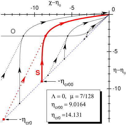
Figure 8: Global view of the relativistic phase trajectories of a test ion with $\mu=7/128$. Depending on the ion start delay $\bar{t}_{p0}\geq 0$, the starting point of each trajectory may lie anywhere between its intersection with the grey thick curve $O$, defined by Eqs. (50), and with the bisector $\eta=\chi$ (dashed line). Straight dotted segments of the phase trajectories correspond to ion acceleration inside the vacuum gap.

A qualitative difference between the relativistic and non-relativistic cases arises when one considers the behavior of the separatrix $S$. In the non-relativistic limit the latter is a straight line given by Eq. (49a). Therefore, all physically interesting ion trajectories that start from $x_{p}=0$ with the zero initial velocity $v_{p}=0$ at any time $t_{p0}\geq 0$ always lie below $S$, i.e. belong to the first class described in the previous paragraph. The relativistic separatrix, in contrast, bends down and crosses the line $\eta=\chi$ at a certain value $\eta-\eta_{0}=\chi-\eta_{0}=-\eta_{cr00}$ (see Fig. 8), where $\eta_{cr00}=\eta_{cr00}(\mu)$ is a function of $\mu$. As a consequence, for a given $\mu$ and $\eta_{0}>\eta_{cr00}(\mu)$ the phase trajectory of a test ion may pass above the separatrix and fall into the second class. In such a case a test ion overtakes the electron front within a finite time interval. To reach more definite conclusions, we have to take a closer look at the initial conditions.

If a test ion begins to move simultaneously with electrons at $t=t_{p0}=0$, the initial part of its trajectory lies in vacuum and is represented by a segment of a straight line $\eta=\eta_{vac}(\chi)=2\chi$ [as it follows from Eqs. (39) and (46)] with $0\leq\chi\leq\chi_{p1}=\frac{1}{2}\eta_{p1}$; in Fig. 8 these segments are shown as dotted straight intervals. Then, the initial conditions for the phase equation (48) are given by the values

$$\chi=\chi_{p1}=\frac{1}{2}\eta_{p1},$$ (50a)

$$\eta=\eta_{p1}=\textrm{arcsinh}\left[\frac{2\mu\sinh\eta_{0}\,\left(1+\mu\cosh\eta_{0}\right)}{1+2\mu\cosh\eta_{0}+\mu^{2}}\right]\!,$$ (50b)

inferred from Eqs. (39), (40) and (46). If we fix $\mu$ and treat $\eta_{0}$ as a free parameter, Eqs. (50) define a universal curve $O$, the locus of the initial points for the integral curves of Eq. (48) in the $(\chi-\eta_{0},\eta-\eta_{0})$ plane (see Fig. 8). The value of parameter $\eta_{0}$ along the curve $O$ at its intersection with the separatrix $S$ defines the primary critical value $\eta_{cr0}=\eta_{cr0}(\mu)$ for this parameter. Its meaning is as follows: for any $\eta_{0}>\eta_{cr0}(\mu)$ a test ion with the charge-over-mass ratio $\mu$ finally catches up with the electron front and overtakes it.

The fact that the vacuum segments of the phase trajectories in Fig. 8 rise less steeply than the initial portions of the relativistic integral curves of Eq. (48) implies that a delayed (at $t_{p0}>0$) start of a test ion may result in its more efficient acceleration. In reality such a delayed start may occur when a test positive particle is created on the spot some time after the laser pulse. If we consider a delayed start at $\bar{t}_{p0}\geq 2$, when the vacuum gap is already closed (the opposite extreme to the previously considered case of simultaneous start at $t_{p0}=0$), the locus of the initial points $(\chi,\eta)=(0,0)$ for the integral curves of Eq. (48) in the $(\chi-\eta_{0},\eta-\eta_{0})$ plane will be the bisector line $\eta-\eta_{0}=\chi-\eta_{0}$. Hence, the intersection of the separatrix $S$ with this bisector defines the secondary critical value $\eta_{cr00}=\eta_{cr00}(\mu)<\eta_{cr0}(\mu)$ of parameter $\eta_{0}$ (see Fig. 8) which has the following meaning: for any $\eta_{0}<\eta_{cr00}(\mu)$ a test ion with the charge-over-mass ratio $\mu$ always stays behind the electron front for all possible starting times $t_{p0}\geq 0$ . In the intermediate case of $\eta_{cr00}<\eta_{0}<\eta_{cr0}$ a test ion can either overtake the electron front or stay behind it, depending on the start delay $0<\bar{t}_{p0}<2$. A selection of $\eta_{cr0}(\mu)$ and $\eta_{cr00}(\mu)$ values calculated by solving Eq. (48) numerically is given in Table 1.

Table 1: Critical parameters $\eta_{cr0}(\mu)$, $\eta_{cr00}(\mu)$, and $\eta_{cr\Lambda}(\mu)$ as calculated for a selection of $\mu$ values by numerically integrating the ion equations of motion (47).

$1/\mu$	$\eta_{cr0}$	$\eta_{cr00}$	$\eta_{cr\Lambda}$
10	5.94216	4.51193	5.35497
20	15.7848	9.88926	15.0917
100	94.3602	49.9827	93.6670
200	193.685	99.9916	192.990
1000	992.089	499.998	991.395
2000	1991.40	999.999	1990.71

IV.1.4 The ultra-relativistic limit

In the physically important limit of $\mu\ll 1$ the functions $\eta_{cr0}(\mu)$ and $\eta_{cr00}(\mu)$ can be calculated analytically by using the ultra-relativistic ($\mu\Pi_{0}\gg 1$) expansion of Eqs. (50) for the curve $O$ in Fig. 8,

$$\eta-\eta_{0}=\ln\mu,$$ (51)

and the integral

$$\exp\left(\eta-\eta_{0}\right)-2\mu(\chi-\eta_{0})=C$$ (52)

of Eq. (48) in the limit of $\eta_{0}-\chi\gg 1$, $\eta-\chi\gg 1$, when the right-hand side of Eq. (48) can be approximated as $2\mu\exp(\eta_{0}-\eta)$. Having set the integration constant $C=1$, we obtain the equation of the separatrix $S$ in the $(\chi-\eta_{0},\eta-\eta_{0})$ plane. Note that, although derived in the limit of $\eta_{0}-\chi\gg 1$, this equation has a correct limiting behavior at $\chi\to\eta_{0}$ as well. After we calculate the intersection points of the separatrix $S$ with the curve $O$ [as given by Eq. (51)] and with the bisector $\chi=\eta$, we find

$$\eta_{cr0}=\ln\mu+\frac{1}{\mu}-1, \gamma_{cr0}=\frac{1}{2}\,\mu\,\exp\left(\frac{1}{\mu}-1\right),$$ (53)

$$\eta_{cr00}=\frac{1}{2\mu}, \gamma_{cr00}=\frac{1}{2}\exp\left(\frac{1}{2\mu}\right).$$ (54)

The corresponding critical values $\gamma_{cr0}(\mu)$ and $\gamma_{cr00}(\mu)$ of the parameter $\gamma_{0}$ are obtained by applying the ultra-relativistic formula $\gamma=\cosh\eta\approx\frac{1}{2}\exp\eta$. Comparison with the numerical results from Table 1 shows that for $\mu^{-1}>20$ the asymptotic formulae (53), (54) for $\eta_{cr0}$ and $\eta_{cr00}$ are accurate to within 1.4%.

Making use of the integral (52) with the values of $C=\exp(\eta_{\infty}-\eta_{0})>1$, we calculate the limiting value $\gamma_{p\infty}=\frac{1}{2}\exp\eta_{\infty}$ of the ion gamma-factor in the case when the ion overtakes the electron front,

$$\gamma_{p\infty}=\left\{\begin{array}[]{ll}\!\mu\gamma_{0}\left(1+\displaystyle\ln\frac{2\gamma_{0}}{\mu}\right),&\textrm{$\bar{t}_{p0}=0$ and $\gamma_{0}>\gamma_{cr0}(\mu)$},\\ \!2\mu\gamma_{0}\,\ln(2\gamma_{0}),&\textrm{$\bar{t}_{p0}\geq 2$ and $\gamma_{0}>\gamma_{cr00}(\mu)$}.\end{array}\right.$$ (55)

This our result for $\gamma_{p\infty}$ differs significantly from the value $\gamma_{p\infty}=2\gamma_{0}^{2}$ calculated earlier in Eq. (35) of Ref. BuEs.04 , which we believe to be erroneous. It should be noted, however, that Eq. (55) can hardly be of any practical interest for protons and heavier ions because for $\mu\leq 1/1836$ the corresponding values of $\gamma_{cr0}\geq 2.3\times 10^{793}$ and $\gamma_{cr00}\geq 2.4\times 10^{398}$ are way too large to be ever encountered in nature.

IV.1.5 Intermediate asymptotics for the ion energy

Having established that in reality test ions of common interest, i.e. those with $\mu\leq 1/1836$, always stay behind the electron front, and that their dimensionless momentum $\Pi_{p}(\bar{t})$ approaches the electron value $\Pi_{0}$ on an unrealistically long timescale $\bar{t}_{ac}\simeq\exp\left(\frac{1}{2}\mu^{-1}\right)$, a natural step would be to look for an intermediate asymptotics for $\Pi_{p}(\bar{t})$, valid at $1\ll\bar{t}\ll\exp\left(\frac{1}{2}\mu^{-1}\right)$, that might be of practical interest for the problem considered.

Once we let $\mu\ll 1$ and agree that $\gamma_{0}\ll\gamma_{cr00}(\mu)<\gamma_{cr0}(\mu)$, we can integrate Eq. (47b) in the limit of $\bar{t}\gg 1$ by making an approximation $\eta=\chi$, which is valid to the first order in $\mu$ along the direction of general approach (49b) to the singular point $(\chi,\eta)=(\eta_{0},\eta_{0})$. With the initial condition

$$\eta(\zeta_{p1})=\eta_{p1},\quad\sinh\eta_{p1}=\Pi_{p1}=\mu\Pi_{0}\bar{t}_{p1},$$ (56)

where $\zeta_{p1}=\ln\bar{t}_{p1}$ and $\bar{t}_{p1}$ is given by Eq. (40), the result of this integration reads

$$\tanh\frac{\eta-\eta_{0}}{2}=\tanh\frac{\eta_{p1}-\eta_{0}}{2}\,\exp\left[-2\mu(\zeta-\zeta_{p1})\right].$$ (57)

Performing Taylor expansion of Eq. (57) with respect to the small parameter $0<2\mu(\zeta-\zeta_{p1})\ll 1$, we derive the following asymptotic expression for the test ion momentum $\Pi_{p}(t)$

$$\frac{\gamma_{p}+\Pi_{p}}{\gamma_{p1}+\Pi_{p1}}=1+\left(\frac{\gamma_{0}+\Pi_{0}}{\gamma_{p1}+\Pi_{p1}}-\frac{\gamma_{p1}+\Pi_{p1}}{\gamma_{0}+\Pi_{0}}\right)\,\mu\ln\frac{t}{t_{p1}},$$ (58)

where $\gamma_{p}=\left(\Pi_{p}^{2}+1\right)^{1/2}$ and $\gamma_{p1}=\left(\Pi_{p1}^{2}+1\right)^{1/2}$. Note that, once $1\ll\bar{t}\ll\exp\left(\frac{1}{2}\mu^{-1}\right)$, Eq. (58) applies at any degree of relativism of either electrons or a test ion, i.e. any of the three quantities $\Pi_{0}$, $\Pi_{p1}$, and $\Pi_{p}$ is allowed to be arbitrarily small or large compared to unity. Comparison with numerical integration of Eqs. (47) shows that for $\mu\leq 1/1836$ the error of the intermediate asymptotics (58) at $1\leq\ln(t/t_{p1})\leq 50$ is typically about 2–4%, and never exceeds 8%. In both the non-relativistic ($\Pi_{0}\ll 1$) and the ultra-relativistic ($\mu\Pi_{0}\gg 1$) limits Eq. (58) reduces to a simple expression

$$\Pi_{p}\approx\Pi_{p1}\left(1+\ln\frac{t}{t_{p1}}\right).$$ (59)

IV.2 Solution for $\Lambda>h_{0}$

From practical point of view the case of $\Lambda\gtrsim 1$ is generally more important than the limit $\Lambda=0$ considered so far. As a typical example, it may be noted that a 1 ${}\mu$m foil of solid gold ionized to $z=50$ with $\gamma_{0}=100$ would correspond to $\Lambda\approx 10$. Here we prove that practically all the qualitative and many of the quantitative results obtained for $\Lambda=0$ extend to the case of $\Lambda>0$ as well. To avoid unnecessary mathematical complications, we exclude from our consideration the intermediate range of $0<\Lambda<h_{0}$ and assume that $\Lambda>h_{0}=\left[2\gamma_{0}/(1+\gamma_{0})\right]^{1/2}$.

In units (25) the equations of ion motion (38) become

$$\beta_{0}\frac{d\tilde{x}_{p}}{d\tilde{t}} = \frac{\Pi_{p}}{\sqrt{1+\Pi_{p}^{2}}},$$ (60a)

$$\frac{d\Pi_{p}}{d\tilde{t}} = \mu\Pi_{0}\,\tilde{l}(\tilde{t},\tilde{x}_{p},\beta_{0}).$$ (60b)

As discussed in section III.3, the function $\tilde{l}(\tilde{t},\tilde{x},\beta_{0})$ does not depend on $\Lambda$ at $\Lambda>h_{0}$, and is a smooth function of its arguments in the entire region $0\leq\tilde{t}<\infty$, $0\leq\tilde{x}\leq\tilde{t}$. In the case of a simultaneous ion start at $t_{p0}=0$ we have the initial conditions $\tilde{x}_{p}(0)=\Pi_{p}(0)=0$, and the leading terms in expansion of the desired solution to Eqs. (60) near $\tilde{t}=0$ are given by

$$\tilde{x}_{p}(\tilde{t}) = \frac{1}{6}\mu\gamma_{0}\,\tilde{t}^{3}+O(\tilde{t}^{4}),$$ (61a)

$$\Pi_{p}(\tilde{t}) = \frac{1}{2}\mu\Pi_{0}\,\tilde{t}^{2}+O(\tilde{t}^{3}).$$ (61b)

Since neither Eqs. (60) nor the pertinent boundary conditions depend on $\Lambda$, we arrive at an important conclusion that, when expressed in units (25), all the results concerning test ion acceleration in the laminar zone are independent of $\Lambda$ for $\Lambda>h_{0}$.

The next important point is that in the limit of $\tilde{t}\to\infty$ equations (60) become exactly equivalent to the corresponding equations of motion for $\bar{x}_{p}(\bar{t})$, $\Pi_{p}(\bar{t})$ in the case of $\Lambda=0$. To verify this, we note that Eqs. (30)-(35) imply $\tilde{l}\sim 2/\tilde{t}\ll 1$ for $\tilde{t}\gg 1$. Then, by expanding Eqs. (30)-(35) in powers of $\tilde{l}$, we derive an explicit formula

$$\tilde{l}(\tilde{t},\tilde{x},\beta_{0}) \approx 4(\tilde{t}-\tilde{x})\left\{\tilde{t}^{2}-\beta_{0}^{2}\tilde{x}^{2}+2+\vphantom{\left[(\tilde{t}^{2}-2)\right]^{1/2}}\right.$$ (62)

$$\left.\left[(\tilde{t}^{2}-\beta_{0}^{2}\tilde{x}^{2}-2)^{2}+8(1-\beta_{0}^{2})\tilde{t}\tilde{x}\right]^{1/2}\right\}^{-1}\!\!\!\!,$$

which is valid for any $0<\beta_{0}<1$ in the limit of $\tilde{l}\ll 1$, and which is further simplified to

$$\tilde{l}(\tilde{t},\tilde{x},\beta_{0})\approx\frac{2(\tilde{t}-\tilde{x})}{\tilde{t}^{2}-\beta_{0}^{2}\tilde{x}^{2}}$$ (63)

for $\tilde{t}\gg\gamma_{0}$ and all $0\leq\tilde{x}\leq\tilde{t}$. Substituting Eq. (63) into Eq. (60b), we obtain exactly the same equations with respect to $\tilde{x}_{p}(\tilde{t})$, $\Pi_{p}(\tilde{t})$ as those with respect to $\bar{x}_{p}(\bar{t})$, $\Pi_{p}(\bar{t})$ in section IV.1, which are then reduced to the same phase equation (48) with the same topology of integral curves in the vicinity of the singular point $(\chi,\eta)=(\eta_{0},\eta_{0})$. As a consequence, we arrive at conclusions that are fully analogous to those made for the case of $\Lambda=0$:

• test ions with $\mu>\mu_{\ast}=\frac{1}{8}$ always catch up and overtake the electron front, being finally accelerated to $\Pi_{p\infty}>\Pi_{0}$;

• for any $\mu<\frac{1}{8}$ there exists a critical value $\eta_{cr\Lambda}(\mu)$ of parameter $\eta_{0}$ [or, equivalently, a critical value $\gamma_{cr\Lambda}(\mu)$ of parameter $\gamma_{0}$] such that only for $\eta_{0}>\eta_{cr\Lambda}(\mu)$ [i.e. for $\gamma_{0}>\gamma_{cr\Lambda}(\mu)$] can a test ion with the charge-over-mass ratio $\mu$ overtake the electron front and be accelerated to $\Pi_{p\infty}>\Pi_{0}$; for $\eta_{0}<\eta_{cr\Lambda}(\mu)$ a test ion lags behind the electron front while its dimensionless momentum $\Pi_{p}(\tilde{t})$ asymptotically approaches $\Pi_{0}$ on a timescale $\tilde{t}_{ac}\simeq\exp\left(\frac{1}{2}\mu^{-1}\right)$.

These conclusions are fully confirmed by numerical integration of Eqs. (60) with $\tilde{l}(\tilde{t},\tilde{x},\beta_{0})$ calculated from Eqs. (30)-(35).

A remarkable fact is that we have two universal functions, namely, $\eta_{cr0}(\mu)$ for $\Lambda=0$, and $\eta_{cr\Lambda}(\mu)$ for $\Lambda>h_{0}$, which cover the entire range of $\Lambda$ variation. Since at intermediate times $\tilde{t}\simeq 1$ the two cases of $\Lambda=0$ and $\Lambda>h_{0}$ are mathematically not equivalent, the functions $\eta_{cr0}(\mu)$ and $\eta_{cr\Lambda}(\mu)$ numerically differ from one another, except for the initial point $\eta_{cr0}(\mu_{\ast})=\eta_{cr\Lambda}(\mu_{\ast})=0$. This difference, however, is practically not significant, as one verifies by comparing the numerically calculated values of $\eta_{cr0}(\mu)$ and $\eta_{cr\Lambda}(\mu)$ in Table 1. In the limit of $\mu\ll 1$ one derives an asymptotic expression

$$\gamma_{cr\Lambda}=\frac{1}{4}\mu\,\exp\left(\frac{1}{\mu}-1\right),$$ (64)

which is exactly one half of the corresponding limit (53) for $\gamma_{cr0}$. One can safely conjecture that for intermediate values $0<\Lambda<h_{0}$ the corresponding critical values of $\gamma_{0}$ lie between $\gamma_{cr0}(\mu)$ and $\gamma_{cr\Lambda}(\mu)$. For $\gamma_{0}>\gamma_{cr\Lambda}(\mu)$, when a test ion does overtake the electron front, its final energy in the limit of $\mu\ll 1$ is given by

$$\gamma_{p\infty}=\mu\gamma_{0}\left(1+\ln\frac{4\gamma_{0}}{\mu}\right).$$ (65)

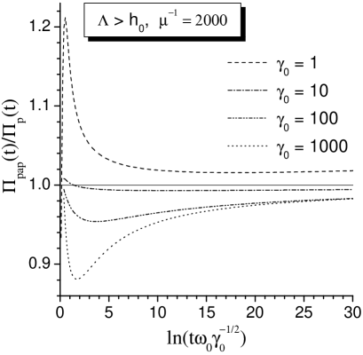
Figure 9: Comparison of the intermediate asymptotics (58) with the results of numerical integration of the ion equations of motion (60) for $\mu=1/2000$ and four different values of $\gamma_{0}$: plotted is the ratio of the ion momentum $\Pi_{pap}(t)$, obtained from Eqs. (58) and (66), to the numerically calculated value $\Pi_{p}(t)$ versus time $t$ in units (25).

Under the approximation (63) one derives the same intermediate asymptotics (58) for the test ion momentum $\Pi_{p}(t)$ as in the case of $\Lambda=0$. The only difference between the two cases is in the initial values of $t_{p1}$ and $\Pi_{p1}=\Pi_{p}(t_{p1})$ to be used in Eq. (58). Unlike in the $\Lambda=0$ case, no appropriate analytical solution to Eqs. (60) was found for $\tilde{t}\lesssim 1$ that would yield suitable expressions for $\tilde{t}_{p1}$ and $\Pi_{p1}$. It is only in the ultra-relativistic limit $\mu\Pi_{0}\gg 1$ that one obtains a simple result $\Pi_{p1}=\mu\Pi_{0}$, $\tilde{t}_{p1}=\left(\frac{1}{2}\mu\gamma_{0}\right)^{1/2}$. In the opposite limit of $\mu\Pi_{0}\ll 1$ expansion (61b) suggests that the value $\Pi_{p}=\mu\Pi_{0}$ is achieved at $\tilde{t}\simeq 1$. Taking guidance from such considerations, we propose simple approximate expressions

$$\Pi_{p1}=\mu\Pi_{0},\quad\tilde{t}_{p1}=\left(2+\frac{1}{2}\mu\gamma_{0}\beta_{0}^{2}\right)^{1/2},$$ (66)

which, on the one hand, agree with the ultra-relativistic limit and, on the other hand, fit reasonably well the results of numerical integration of Eqs. (60) shown in Fig. 9. As a result, Eq. (58) with $\Pi_{p1}$ and $\tilde{t}_{p1}$ taken from Eq. (66) is formally applicable at $\tilde{t}_{p1}\ll\tilde{t}\ll\exp\left(\frac{1}{2}\mu^{-1}\right)$. A comparison with numerical results in Fig. 9 shows that at $\tilde{t}\gtrsim 100$ the intermediate asymptotics (58) has a typical error of a few percent.

If we consider now the case of a delayed ion start at $t=t_{p0}>0$, we find that for $\tilde{t}_{p0}\gg 1$ we have $\tilde{l}\ll 1$ for all $\tilde{t}\geq\tilde{t}_{p0}$, which again leads us to the approximation (63) and to the phase equation (48) with the initial condition $(\chi,\eta)=(0,0)$. Hence, exactly as in the $\Lambda=0$ case, the critical value of the $\eta_{0}$ parameter for $\tilde{t}_{p0}\gg 1$ should be given by the function $\eta_{cr00}(\mu)$. This conclusion is also fully confirmed by numerical integration of Eqs. (60). For $\mu\ll 1$ the dependence of the critical $\eta_{0}$ on the ion start delay $\tilde{t}_{p0}$ is as follows: as $\tilde{t}_{p0}$ increases from $\tilde{t}_{p0}=0$ to $\tilde{t}_{p0}=\sqrt{2}$, the critical value of $\eta_{0}$ decreases from $\eta_{cr\Lambda}(\mu)$ to $\eta_{cr00}(\mu)$, and for $\tilde{t}_{p0}>\sqrt{2}$ it remains equal to $\eta_{cr00}(\mu)$.

IV.3 Domain of applicability of the laminar-zone solution

The foregoing analysis of test ion acceleration has been based on the assumption that the ion trajectories lie entirely inside the laminar zone of the electron sheath. As already mentioned in section III, this is true only within a certain domain of our three-dimensional parameter space $(\mu,\gamma_{0},\Lambda)$. Because of a weak dependence on $\Lambda$, the limits of this domain can be conveniently analyzed in the two-dimensional $(\mu^{-1},\eta_{0})$ plane.

Let $\eta_{lam}(\mu)$ be the threshold value of $\eta_{0}=\textrm{arccosh}\,\gamma_{0}$ at which the trajectory of an ion with a given charge-over-mass ratio $\mu$ just touches the outer boundary of the relaxation zone (see Figs. 5 and 6), i.e. for $\eta_{0}>\eta_{lam}(\mu)$ the ion trajectory lies entirely in the laminar zone, and for $\eta_{0}<\eta_{lam}(\mu)$ it penetrates (at least partially) into the relaxation zone. Typically this touching occurs near the first local maximum of the corresponding $\chi_{r}(t)$ curve at $\bar{t},\tilde{t}\simeq 15$–20 and lies within the reach of the TIAC code. Because this early part of the boundary between the two zones ceases to depend on $\Lambda$ for $\Lambda\gtrsim 2.5$, the same applies to the function $\eta_{lam}(\mu)$.

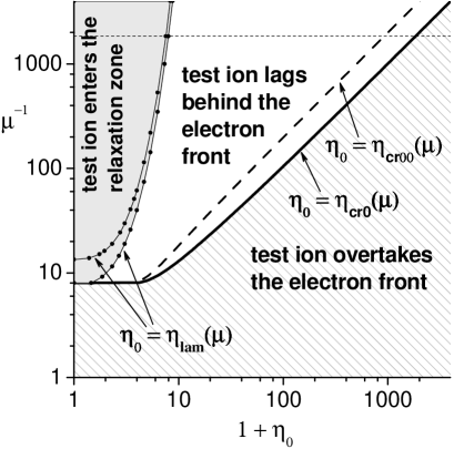
Figure 10: Characteristic regions in the $(\eta_{0},\mu^{-1})$ parameter plane. Domain of applicability of the laminar-zone solution lies outside the grey shaded area delimited by the two $\eta_{lam}(\mu)$ curves, the inner one calculated for $\Lambda=0$, and the outer one for $\Lambda=10$. Hatched region is where test ions overtake the electron front: it is delimited by the $\eta_{cr0}(\mu)$ curve which is practically indistinguishable from $\eta_{cr\Lambda}(\mu)$. Dashed horizontal line corresponds to the proton value $\mu^{-1}=1836$.

Figure 10 shows two curves $\eta_{lam}(\mu)$, calculated for $\Lambda=0$ and 10, which actually span the entire dependence of $\eta_{lam}$ on the $\Lambda$ parameter. The domain of applicability of the laminar-zone results lies outside the grey shaded area bounded by the $\eta_{lam}(\mu)$ curves. For protons with $\mu=1/1836$ it corresponds to $\gamma_{0}>348$ at $\Lambda=0$, and to $\gamma_{0}>537$ at $\Lambda\gtrsim 2.5$. The fact that the two critical values $\eta_{cr0}(\mu)$ and $\eta_{cr00}(\mu)$ turn out to be deeply inside this domain (at least for $\mu<0.1$) justifies all the conclusions made in sections IV.1 and IV.2 about the possibility for a test ion to catch up with the electron front. Note that the two curves $\eta_{cr0}(\mu)$ and $\eta_{cr\Lambda}(\mu)$, which span the dependence of the critical value $\eta_{cr}$ on the $\Lambda$ parameter, are virtually indistinguishable in Fig. 10.

For protons and heavier ions with $\mu\leq 1/1836$ the following conclusions can be drawn from Fig. 10. The position of the $\eta_{lam}(\mu)$ curves indicates that ion acceleration in the non-relativistic case of $\Pi_{0}\ll 1$ takes place deeply in the relaxation zone, where one can expect the usual Boltzmann relation to be a good approximation. The laminar-zone solution is not applicable in such a case. However, it becomes fully applicable when the electrons are boosted to highly relativistic energies of $\gamma_{0}\gtrsim 300$–500 ($\eta_{0}\gtrsim 6$–7).

V Conclusion

In this paper rigorous results are presented for a particular case of the TNSA mechanism of ion acceleration in a planar electron sheath evolving from an initially mono-energetic cloud of hot electrons. Self-consistent treatment of the collisionless electron dynamics fully captures the effects of departure from the Maxwell-Boltzmann distribution. These effects come to a foreground in the outer laminar zone of the expanding electron cloud, where the ion acceleration can be analyzed by analytical means. In particular, the limiting (in the limit of $t\to\infty$) gamma-factor $\gamma_{p\infty}$ of an accelerated test ion can be calculated exactly. Note that the assumption of an isothermal Boltzmann distribution for hot electrons leads to an infinite value of $\gamma_{p\infty}$.

It is shown that the limiting value $\gamma_{p\infty}$ is determined primarily by the values of the two (out of the total three) principal dimensionless parameters of the problem, the ion-electron charge-over-mass ratio $\mu=m_{e}Z_{p}/m_{p}$, and the initial gamma-factor $\gamma_{0}$ of the accelerated electrons. For $\mu>\mu_{\ast}=\frac{1}{8}$ a test positive particle (for example a positron) always overtakes the electron front and reaches $\gamma_{p\infty}>\gamma_{0}$. In the physically more interesting case of $\mu<\mu_{\ast}$ the limiting ion energy depends on whether $\gamma_{0}$ is above or below a certain critical value $\gamma_{cr}=\gamma_{cr}(\mu)$, namely, we have $\gamma_{p\infty}=\gamma_{0}$ for $\gamma_{0}<\gamma_{cr}$, and $\gamma_{p\infty}>\gamma_{0}$ [as given by Eqs. (55) and (65)] for $\gamma_{0}>\gamma_{cr}$. Practically insignificant dependence of $\gamma_{cr}$ on the dimensionless foil thickness $\Lambda$ is limited to a variation within a factor 2 and spanned by the functions $\gamma_{cr0}(\mu)$ and $\gamma_{cr\Lambda}(\mu)$ calculated in Table 1 and Eqs. (53) and (64).

For protons and heavier ions with $\mu\leq 1/1836$ we always have $\gamma_{0}<\gamma_{cr}$ because the corresponding values of $\gamma_{cr}\sim\exp(\mu^{-1})$ are enormous and beyond practical reach. Therefore, in reality these ions can never catch up with the electron front. Although formally the ion gamma-factor $\gamma_{p}(t)$ in this case still tends to $\gamma_{0}$ as $t\to\infty$, this fact is also practically irrelevant because $\gamma_{p}(t)$ approaches $\gamma_{0}$ on an enormous timescale $t_{ac}\simeq t_{\Sigma}\exp\left(\frac{1}{2}\mu^{-1}\right)$ [or $t_{ac}\simeq\omega_{0}^{-1}\sqrt{\gamma_{0}}\,\exp\left(\frac{1}{2}\mu^{-1}\right)$ for $\Lambda>1$] that never occurs in nature. For practical applications one should use the intermediate asymptotic formula (58) derived for dimensionless times $1\ll\bar{t},\tilde{t}\ll\exp\left(\frac{1}{2}\mu^{-1}\right)$.

Our results for ion motion have been obtained under the condition that the ion trajectory lies entirely in the laminar zone of the electron sheath. Numerical investigation of the evolution of the laminar zone boundaries reveals that this condition imposes a lower bound $\gamma_{0}>\gamma_{lam}(\mu)$ on the initial gamma-factor of hot electrons (see Fig. 10). The latter inequality reflects a more general fact that the role of the non-Boltzmann effects in ion acceleration increases with $\gamma_{0}$, i.e. with the energy of hot electrons. In particular, acceleration of protons by a non-relativistic electron sheath occurs practically entirely in the quasi-Boltzmann core of the electron cloud, where the details of the initial electron energy distribution are “forgotten”. However, in the ultra-relativistic case of mono-energetic electrons with $\gamma_{0}\gtrsim 300$–500, acceleration of protons takes place entirely in the non-Boltzmann laminar zone of the electron sheath, where full memory of the initial electron energy distribution has been preserved.

- (1) E.L. Clark et al., Phys. Rev. Lett. 84, 670 (2000); 85, 1654 (2000).
- (2) A. Maksimchuk et al., Phys. Rev. Lett. 84, 4108 (2000).
- (3) R.A. Snavely et al., Phys. Rev. Lett. 85, 2945 (2000).
- (4) M. Hegelich et al., Phys. Rev. Lett. 89, 085002 (2002).
- (5) T.E. Cowan et al., Phys. Rev. Lett. 92, 204801 (2004).
- (6) G.A. Mourou, T. Tajima, and S.V. Bulanov, Rev. Mod. Phys. 78, 309 (2006).
- (7) S.P. Hatchett et al., Phys. Plasmas 7, 2076 (2000).
- (8) S.C. Wilks et al., Phys. Plasmas 8, 542 (2001).
- (9) A.V. Gurevich, L.V. Pariiskaya, and L.P. Pitaevskii, Zh. Eksp. Teor. Fiz. 49, 647 (1965) [Sov. Phys. JETP 22, 449 (1966)].
- (10) P. Mora, Phys. Rev. Lett. 90, 185002 (2003).
- (11) S. Gitomer et al., Phys. Fluids 29, 2679 (1986).
- (12) J.E. Crow, P.L. Auer, and J.E. Allen, J. Plasma Phys. 14, 65 (1975).
- (13) M. Passoni, V.T. Tikhonchuk, M. Lontano, and V.Yu. Bychenkov, Phys. Rev. E 69, 026411 (2004).
- (14) J.S. Pearlman and R.L. Morse, Phys. Rev. 40, 1652 (1978).
- (15) Y. Kishimoto et al., Phys. Fluids 26, 2308 (1983).
- (16) M. Passoni and M. Lontano, Laser and Part. Beams 22, 163 (2004).
- (17) S.V. Bulanov et al., Plasma Phys. Rep. 30, 18 (2004).