Near-field enhancement and sub-wavelength imaging in the optical region using a pair of two-dimensional arrays of metal nanospheres

Abstract

Near-field enhancement and sub-wavelength imaging properties of a system comprising a coupled pair of two-dimensional arrays of resonant nanospheres are studied. The concept of using two coupled material sheets possessing surface mode resonances for evanescent field enhancement is already well established in the microwave region. This paper shows that the same principles can be applied also in the optical region, where the performance of the resonant sheets can be realized with the use of metallic nanoparticles. In this paper we present design of such structures and study the electric field distributions in the image plane of such superlens.

I Introduction

Recently, there have been many studies of near-field enhancement and sub-wavelength imaging using metamaterial slabs with negative permittivity and permeability (double-negative or DNG media). The predicted negative refraction,Veselago which occurs at an interface between double-positive (DPS, positive permittivity and permeability) and DNG media, was confirmed experimentally in the microwave domain using arrays of split rings and wiresShelby ; Parazzoli ; Houck and also using meshes of loaded transmission lines.Eleftheriades ; Caloz Also, the predicted enhancement of evanescent modesPendry was experimentally confirmed.Grbic ; Alitalo2 A lot of effort is devoted to realization of DNG-slab superlenses in the optical region.Zhou ; Dolling ; Kildishev ; Zhang ; Gabitov ; Alu However, there are many obstacles on this way, due to fundamental difficulties in realization of artificial magnetic materials in the optical region with the use of nano-sized resonant particles.

An alternative approach to the realization of superlenses for evanescent fields has been suggested in Ref. 16. This approach is based on the use of a pair of coupled resonant arrays or resonant sheets placed in a usual double-positive medium, e.g. free space or a dielectric. Systems comprising coupled pairs of arrays of resonant metal particles have been used to demonstrate experimentally the sub-wavelength imaging properties at microwave frequencies.Maslovski ; Freire ; Alitalo3 The main advantage of this route to superlens design is that a superlens with sub-wavelength resolution can be realized without using a bulk DNG medium. Only two sheets supporting surface modes in a broad spectrum of spatial frequencies are required, if enhancement of only evanescent modes is desired (although the propagating modes in this case are not focused in the image plane as with a bulk DNG slab, the imaging is still possible Maslovski ; Freire ; Alitalo3 ). Removal of the bulk DNG slab strongly mitigates the problem of losses that have been present in any realized DNG medium so far.

The goal of the present work is to show that sub-wavelength imaging characteristics in a device based on resonant arrays can be achieved also at very high frequencies (the optical region and above) if we use metallic nano-sized particles as the resonating inclusions of the two arrays. This approach to the realization of an optical superlens was first suggested in Ref. 19. In this paper we will study the dispersion in two-dimensional arrays of silver and gold nanospheres and show that the dispersion characteristics are suitable for using these types of arrays for evanescent field enhancement. Next, the electric field distributions in a superlens consisting of two arrays of metal nanospheres are studied numerically, in order to confirm and analyze the sub-wavelength resolution of the image formed by the lens.

II Structure of the lens and dispersion in arrays of vertically polarized metal spheres

The structure of the superlens that is studied in this paper is shown in Fig. 1. The spherical particles have the diameter which is considerably smaller than the optical wavelength, and the sphere material is a noble metal. The spheres exhibit a plasmonic resonance within the optical region ($\lambda_{0}=400$ nm…700 nm). The whole structure (including the source and image planes) is embedded in a host medium with the relative permittivity $\varepsilon_{\rm h}$. We will consider the lens to be working properly if we obtain a sub-wavelength image in the image plane with the distance between the source and image planes being larger than $\lambda_{\rm eff}/2$ ($\lambda_{\rm eff}$ is the wavelength in the host medium).

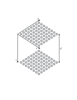
Figure 1: A superlens formed by two planar arrays of spherical metal particles, embedded in a host medium.

The operational principle of the device requires that at the operational frequency each of the two sheets supports surface waves (plasmons) in a wide range of propagation constants along the sheet planes. Existing of eigenmodes with high values of the propagation constant ensures resonant amplification of incident evanescent waves with large values of the transverse wavenumber. This means that for the optimal operation of the superlens we need to design nano-scaled arrays whose dispersion curve is as flat as possible in the vicinity of the operational frequency. Using the approach of Ref. 19, we will first study the dispersion in a single array of the proposed lens. The goal is to find the suitable parameters of the particles and the array period using a simplified model of infinite arrays, which can be further optimized by numerical studies of realistic structures of a finite size. In addition to the assumption of the infinite grid (along $x$ and $y$), in this section we will also assume that each particle is polarized vertically (i.e., the polarization vector is normal to the array surface).

The dispersion in an infinite, two-dimensional array of vertical dipoles can be calculated using the interaction coefficient $C$ of such array:Simovski2

$C=\frac{k^{2}}{4\pi\varepsilon_{\rm h}\varepsilon_{0}}\sum\limits_{m,n=-\infty}^{\infty}\left[1+\frac{j}{kR_{mn}}+\frac{1}{k^{2}R_{mn}^{2}}\right]$

$$\times\frac{e^{-jkR_{mn}}-j\textbf{k}_{t}\cdot\textbf{R}_{mn}}{R_{mn}},$$ (1)

where $k$ is the wavenumber, $k_{t}=\sqrt{k_{x}^{2}+k_{y}^{2}}$ is the transverse wavenumber and $R_{mn}$ is the distance between spheres $m$ and $n$. The inverse polarizability of a metal sphere is (e.g., Ref. 19)

$$\frac{1}{\alpha}=\frac{\varepsilon_{\rm m}+2\varepsilon_{\rm h}}{3\varepsilon_{0}\varepsilon_{\rm h}\frac{4\pi r_{0}^{3}}{3}(\varepsilon_{\rm m}-\varepsilon_{\rm h})}+j\frac{k^{3}}{6\pi\varepsilon_{0}\varepsilon_{\rm h}},$$ (2)

where $\varepsilon_{\rm m}$ is the permittivity of metal and $r_{0}$ is the radius of the sphere. The permittivity of metal can be expressed as:Absorption

$$\varepsilon_{\rm m}=1-\frac{\omega_{p}^{2}}{\omega\left(\omega-j\omega_{D}\right)},$$ (3)

where $\omega_{p}$ and $\omega_{D}$ are the plasma and damping frequencies of the metal, respectively. For lossless particles $\omega_{D}=0$ and the dispersion equation $1/\alpha=C$ transits to the real equationSimovski

$${\rm Re}\left(\frac{1}{\alpha}\right)={\rm Re}(C).$$ (4)

Equation (4) was solved numerically using the fast-converging representation for series (1).Simovski2 By studying the dispersion characteristics of an infinite two-dimensional array, the dimensions of the array (i.e., the radius of the spheres and the period $a$) can be found in such a way that the dispersion curve is reasonably flat while the size of the spheres is of the same order as the period of the arrays.

The parameters of the arrays that are used in this paper are shown in Tables 1 and 2, where the wavelengths $\lambda_{p}$ and $\lambda_{D}$ correspond to the plasma and damping frequencies of the spheres, respectively. Here we have used the plasma and damping frequencies for bulk silver and gold, which is an adequate approximation for the sphere sizes that we are using.Absorption The plasma and damping frequencies for silver have been obtained from Ref. 22 and for gold from Ref. 21. In the calculation of the dispersion curve, we have used $\varepsilon_{\rm h}=1$ for simplicity. The resonant frequency ($f_{\rm r}$) of the spheres that is shown in Tables 1 and 2 is calculated from the plasma frequency with

$$\omega_{r}=\omega_{p}/\sqrt{1+2\varepsilon_{\rm h}}.$$ (5)

Table 1: Parameters of the silver sphere array.

$r_{0}$	$a$	$\lambda_{p}$	$\lambda_{D}$	$f_{\rm r}$ ($\varepsilon_{\rm h}=1$)
28 nm	65 nm	328 nm	58433 nm	$5.2806\cdot 10^{14}$ Hz

Table 2: Parameters of the gold sphere array.

$r_{0}$	$a$	$\lambda_{p}$	$\lambda_{D}$	$f_{\rm r}$ ($\varepsilon_{\rm h}=1$)
15 nm	40 nm	145 nm	11500 nm	$1.1945\cdot 10^{15}$ Hz

With the values shown in Tables 1 and 2, the dispersion curves of the arrays can be plotted using (4), see Figs. 2 and 3. From these results we can conclude that the dispersion curve for both types of metal spheres is reasonably flat in a large range of values of $q$ (where $q=k_{x}/\sqrt{2}=k_{y}/\sqrt{2}$).

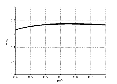
Figure 2: Dispersion of an infinite two-dimensional array of silver nanospheres. Normalized frequency as a function of the normalized transverse wavenumber. The spheres are assumed to be polarized vertically.

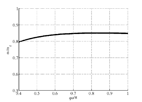
Figure 3: Dispersion of an infinite two-dimensional array of gold nanospheres. Normalized frequency as a function of the normalized transverse wavenumber. The spheres are assumed to be polarized vertically.

III Field distributions in the image plane of the lens

With the suitable array dimensions found in the previous section, it is now possible to study the electric field distributions in a system of two finite two-dimensional arrays of resonant nanospheres. The losses of the metal spheres are taken into account by using complex values for the polarizability of the spheres and the permittivity of the metal. The ideal operation of the lens is illustrated in Fig. 4, where the image (defined in the image plane, i.e., $z=2h+d$) appears as a perfect reconstruction of the source (situated in the plane $z=0$).

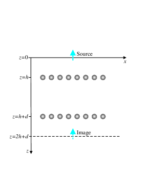
Figure 4: (Color online) Ideal operation of the superlens.

The fields are calculated simply by considering each sphere as having three orthogonal dipole moments at the same frequency (where the dispersion curve is flat) and calculating separately the contribution of each sphere to the image plane field. Because the two arrays of spheres interact, the first task is to solve all the dipole moments $\textbf{P}_{m}$ that correspond to each sphere, taking into account the interaction between all the spheres. This can be done by solving the following equation:

$$\textbf{P}_{m}=\alpha\textbf{E}_{\rm loc}=\alpha\left[\textbf{E}_{m}^{\rm ext}+\sum_{n\neq m}\textbf{E}_{n}\right],$$ (6)

where $\textbf{E}_{\rm loc}$ is the local field acting on the $m$:th sphere, $\textbf{E}_{m}^{\rm ext}$ is the external field (caused by the source) and $\textbf{E}_{n}={\overline{\overline{\Phi}}}_{m,n}\cdot\textbf{P}_{n}$ is the field caused by dipole $\textbf{P}_{n}$. All fields are evaluated at the position of the $m$:th sphere. Here the dyadic function ${\overline{\overline{\Phi}}}_{m,n}$ (with $m\neq n$) describes the interaction between spheres $m$ and $n$. If we introduce the notation

$${\overline{\overline{\Phi}}}_{m,m}=-\frac{1}{\alpha}\overline{\overline{I}},$$ (7)

where $\overline{\overline{I}}$ is the unit dyadic, (6) can be expressed in a simpler form (for each orthogonal component of the vectors separately):

$$\sum_{n}\Phi_{m,n}P_{n}=-E_{m}^{\rm ext}.$$ (8)

The electric field at point ($x$, $y$, $z$) of a dipole with the dipole moment p placed at ($x^{\prime}$, $y^{\prime}$, $z^{\prime}$) is (e.g., Ref. 23)

$\textbf{E}=\frac{1}{4\pi\varepsilon_{\rm h}\varepsilon_{0}}\left\{k^{2}(\textbf{u}\times\textbf{p})\times\textbf{u}\frac{e^{-jkr}}{r}\right\}$

$$+\frac{1}{4\pi\varepsilon_{\rm h}\varepsilon_{0}}\left\{[3\textbf{u}(\textbf{u}\cdot\textbf{p})-\textbf{p}]\left(\frac{1}{r^{3}}+\frac{jk}{r^{2}}\right)e^{-jkr}\right\},$$ (9)

where

$$\textbf{u}=\frac{(x-x^{\prime})\textbf{x}_{0}+(y-y^{\prime})\textbf{y}_{0}+(z-z^{\prime})\textbf{z}_{0}}{r}$$ (10)

and

$$r=\sqrt{(x-x^{\prime})^{2}+(y-y^{\prime})^{2}+(z-z^{\prime})^{2}}.$$ (11)

From (9) we can derive ${\overline{\overline{\Phi}}}_{m,n}$.

Next, let us assume that two finite two-dimensional arrays of spheres are placed in a host medium with permittivity $\varepsilon_{\rm h}$. The distance between the arrays along the $z$-direction is $d$. Also, let us assume that a source, which consists of one or more short vertical electric dipoles, is placed on top of the first array at distance $h$ from the surface of that array. The source excites both arrays, and the $x$, $y$ and $z$-components of the field at the position of each sphere ($E_{m,x}^{\rm ext}$, $E_{m,y}^{\rm ext}$ and $E_{m,z}^{\rm ext}$) can be calculated from (9) by choosing $\textbf{p}=p\textbf{z}_{0}$. The $x$-, $y$-, and $z$-components of $\Phi_{m,n}$ can also be calculated with (9), where $r$ is now the distance from sphere $m$ to $n$. The dipole moments $P_{n,x}$, $P_{n,y}$ and $P_{n,z}$ of each sphere can then be calculated from (8). With the dipole moments solved, (9) can be used to calculate the vertical component of electric field in the image plane caused by all the spheres in the two arrays. To get the total field in the image plane, we must add also the field produced by the source to the field of the arrays.

We have calculated the field distributions in the image plane for different sphere materials (silver and gold) and also for different sources (one or more vertical dipoles in the source plane) using (8) and (9). In the following, we will study arrays with 20 $\times$ 20 silver spheres in each array. The dimensions of the arrays are the same as shown in Table 1, i.e., the radius of the spheres is $r_{0}=28$ nm and the period of the arrays is $a=65$ nm. The dimensions of the lens are $h=a$ and $d=2a$. If we choose the source plane to be at $z=0$, then we plot the image plane field at $z=d+2h=4a$. As the permittivity of the host material we have used $\varepsilon_{\rm h}=2.301$, which corresponds to the permittivity of PMMA (polymethyl methacrylate) dielectric.Lee PMMA is used here due to its very low losses (in fact, we have neglected the losses in the host material to simplify the calculations).

Without any extensive optimization procedure, we have found a suitable frequency of operation to be $1.037f_{\rm r}$ (where $f_{\rm r}\approx 3.8643\cdot 10^{14}$ Hz), which corresponds to the effective wavelength of $\lambda_{\rm eff}\approx 493.52$ nm in the host medium. Comparison of this result with the dispersion curve in Fig. 2 shows a considerable difference in the expected operational frequency. This effect can be explained by the fact that the curve in Fig. 2 is plotted for an infinite array. Indeed, as the number of the spheres in the array increases, the operational frequency is expected to decrease, as in arrays of resonant scatterers.Tretyakovbook At the frequency $1.037f_{\rm r}$, the distance between the source and image planes is $4a=260$ nm $\approx 0.53\lambda_{\rm eff}$.

III.1 Excitation by a single source

First, let us have a look at the electric field distribution in the image plane caused by a point source (a short vertical electric dipole) which is situated in the source plane. In this example, the position of the source dipole is at $x=3a$, $y=0$ (the origin of the coordinate system is now at the center of the arrays in the $xy$-plane). See Fig. 5 for the distribution of the $z$-component of the electric field plotted in the image plane, i.e., in the plane $z=2h+d=4a$. For a more detailed picture of the field distribution, see Fig. 6, where we have plotted the field distributions along the line $y=0$.

From Fig. 6 we can conclude that the half-power width of the “image” is about $0.23\lambda_{\rm eff}$, which clearly confirms the sub-wavelength imaging effect. As can also be seen from Fig. 6, the field in the image plane is very strongly enhanced by the arrays: The field in the image plane without the arrays (dashed line) is negligible compared to the field strength of the image formed by the “lens”.

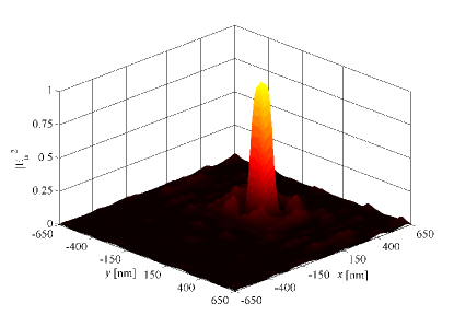
Figure 5: (Color online) Calculated electric field distribution in the image plane with a single source. Fields are normalized to the maximum value.

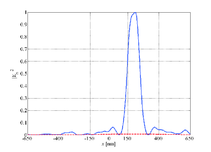
Figure 6: (Color online) Calculated electric field distributions along the line $y=0$ nm in the image plane. Fields are normalized to the maximum value. Solid line: image plane field with the arrays. Dashed line: image plane field without the arrays.

III.2 Excitation by two sources

Next, let us consider excitation by two short vertical dipoles, situated in the source plane. To study the resolution properties of the lens, we place the sources very close to each other. The position of source dipole (1) is $x=1.25a=81.25$ nm, $y=0$ nm and the position of source dipole (2) is $x=-1.25a=-81.25$ nm, $y=0$ nm. With this positioning the distance between sources (1) and (2) is approximately $0.329\lambda_{\rm eff}$. See Fig. 7 for the distribution of the $z$-component of the electric field plotted in the image plane. For a more qualitative picture of the field distribution, see Fig. 8, where we have plotted the field distribution along the line $y=0$.

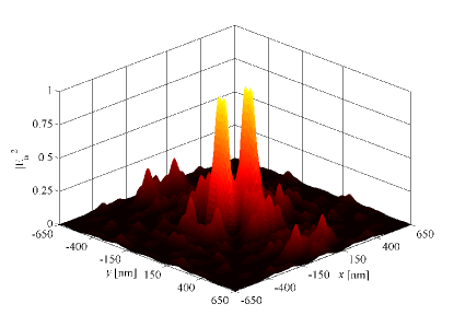
Figure 7: (Color online) Calculated electric field distribution in the image plane with two sources. Fields are normalized to the maximum value.

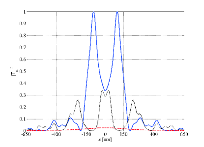
Figure 8: (Color online) Calculated electric field distributions in the image plane. Fields are normalized to the maximum value. Solid line: $y=0$ nm, image plane field with the arrays. Dashed line: $y=0$ nm, image plane field without the arrays. Dotted line: $y=106$ nm, image plane field with the arrays.

From Fig. 8 we can conclude that the two sources can be resolved very reliably (on the level half of the maximum intensity) from the image plane field distribution. As can be seen from Fig. 7, the introduction of multiple sources causes some additional maxima (because of the interference effect), which can potentially hinder the resolution in the image plane. The maximum field corresponding to these unwanted maxima (along line $y=106$ nm) is also plotted in Fig. 8 (dotted line). We see that this maximum is well below the half-power level of the total intensity.

III.3 Effect of the positioning of the sources

The non-symmetric positioning of the sources with respect to the unit cell of the arrays affects the field distributions. The cases studied above relate to the “worst case”, because there the sources are positioned in the center between four neighboring spheres of the arrays (in the $xy$-plane). When a source is positioned directly above a sphere, the maximum of the image will be even more pronounced. Also, when using two sources that are not symmetrically positioned with respect to the unit cell of the arrays (as in the previous subsection), it may happen that the image of the other source has a larger maximum (which corresponds to the fact that this source is closer to a sphere in the $xy$-plane). By studying these special cases it was noticed that the effect of the source positioning is not crucial to the formation of a clear and unambiguous image. The maxima corresponding to the positions of the sources are always above the half-power level.

The effect of the positioning of the sources with respect to the entire sphere array was also studied. It has been noticed that even when using the arrays of 20 $\times$ 20 spheres, the image is properly formed as long as the sources are not very close to the edge of the arrays (in the $xy$-plane). When using two or more sources, the interference maxima grow stronger as the sources get closer to the edge of the arrays.

For an example, see Fig. 9, where two sources are positioned in such a way that the distance from the sources to their closest spheres is different and the both sources are close to the edge of the arrays (in the $xy$-plane). The position of source dipole (1) is $x=4.5a=292.5$ nm, $y=5a=325$ nm and the position of source dipole (2) is $x=2a=130$ nm, $y=5a=325$ nm. With this positioning the distance between the sources is the same as in the above example (approximately $0.329\lambda_{\rm eff}$).

The reason for the difference in the amplitudes of the two “images” in Fig. 9 is not the fact that one source is closer to the edge of the array than the other. The main reason for this is the positioning of the sources with respect to the unit cell of the arrays. However, the interference maximum is affected also by the distance to the edge of the arrays. The dotted line in Fig. 9 corresponds to this interference term of the total field. The maximum of this interference term is somewhat stronger than the one in Fig. 8, and it is due to the placing of the sources near the edge of the arrays.

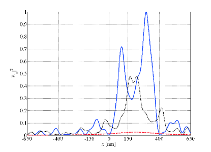
Figure 9: (Color online) Calculated electric field distributions in the image plane. Fields are normalized to the maximum value. Solid line: $y=325$ nm, image plane field with the arrays. Dashed line: $y=325$ nm, image plane field without the arrays. Dotted line: $y=167$ nm, image plane field with the arrays.

III.4 Further improvements of the resolution of the proposed lens

It is possible to further improve the resolution characteristics of the lens studied in this paper. First, the removal of the propagating modes from the lens should mitigate the unwanted interference maxima (this can be realized simply by introducing a thin silver slab between the source plane and the lens). Second way to improve the imaging properties is to introduce a small deviation in the parameters of the arrays (i.e., the radius and the period). This will make the dispersion curve even more flat, with the result that more modes are supported by the arrays. The study of these improvements is beyond the scope of this paper.

IV Conclusions

In this paper we have studied the possibility of using a coupled pair of arrays comprising metallic nanospheres as a near-field imaging device enhancing evanescent fields. We have shown that in arrays with infinitely many silver or gold spheres the dispersion is flat enough so that in a very narrow frequency band most of the evanescent modes are resonantly excited in the arrays. According to the studies made in this paper, this excitation enables the “superlensing” effect, already known in the microwave region, in the optical domain. In the proposed device the enhancement of a large number of the evanescent modes emitted by the source can be realized. We have numerically studied a superlens consisting of two finite arrays of silver spheres and have shown that in the image plane of the lens, resolution better than $\lambda_{\rm eff}/3$ is achievable, even when the distance between the source and image planes is larger than $\lambda_{\rm eff}/2$. According to the results presented in this paper, the use of metallic nanospheres is a very prospective way of extending the use of near-field enhancement phenomenon into the optical region.

References

- (1) V. G. Veselago, Soviet Physics Uspekhi 10, 509 (1968).
- (2) R. A. Shelby, D. R. Smith, and S. Schultz, Science 292 77 (2001).
- (3) C. G. Parazzoli, R. B. Greegor, K. Li, B. E. C. Koltenbah, and M. Tanielian, Phys. Rev. Lett. 90 107401 (2003).
- (4) A. A. Houck, J. B. Brock, and I. L. Chuang, Phys. Rev. Lett. 90 137401 (2003).
- (5) G. V. Eleftheriades, A. K. Iyer, and P. C. Kremer, IEEE Trans. Microwave Theory and Techniques 50 2702 (2002).
- (6) C. Caloz and T. Itoh, IEEE Trans. Antennas and Propagation 52 1159 (2004).
- (7) J. B. Pendry, Phys. Rev. Lett. 85 3966 (2000).
- (8) A. Grbic and G. V. Eleftheriades, Phys. Rev. Lett. 92 117403 (2004).
- (9) P. Alitalo, S. Maslovski, and S. Tretyakov, J. Appl. Phys., 99 124910 (2006).
- (10) J. Zhou, Th. Koschny, M. Kafesaki, E. N. Economou, J. B. Pendry, and C. M. Soukoulis, Phys. Rev. Lett., 95 223902 (2005).
- (11) G. Dolling, C. Enkrich, M. Wegener, C. M. Soukoulis, and S. Linden, Opt. Lett. 31 1800 (2006).
- (12) A. V. Kildishev, W. Cai, U. K. Chettiar, H.-K. Yuan, A. K. Sarychev, V. P. Drachev, and V. M. Shalaev, J. Opt. Soc. Am. B, 23 423 (2006).
- (13) S. Zhang, W. Fan, K. J. Malloy, and S. R. J. Brueck, J. Opt. Soc. Am. B, 23 434 (2006).
- (14) I. R. Gabitov, R. A. Indik, N. M. Litchinitser, A. I. Maimistov, V. M. Shalaev, and J. E. Soneson, J. Opt. Soc. Am. B, 23 535 (2006).
- (15) A. Al and N. Engheta, J. Opt. Soc. Am. B, 23 571 (2006).
- (16) S. Maslovski, S. A. Tretyakov, and P. Alitalo, J. Appl. Phys. 96 1293 (2004).
- (17) M. J. Freire and R. Marques, Appl. Phys. Lett., 86 182505 (2005).
- (18) P. Alitalo, S. Maslovski, and S. Tretyakov, Phys. Lett. A, 357 397 (2006).
- (19) C. R. Simovski, A. J. Viitanen, and S. A. Tretyakov, Phys. Rev. E 72 066606 (2005).
- (20) C. R. Simovski, P. A. Belov, and M. S. Kondratjev, Journal of Electromagnetic Waves and Applications 13 189 (1999).
- (21) C. F. Bohren and D. R. Huffman, Absorption and scattering of light by small particles, John Wiley & Sons, 1983.
- (22) P. B. Johnson and R. W. Christy, Phys. Rev. B 6 4370 (1972).
- (23) S. Tretyakov, Analytical modeling in applied electromagnetics, Norwood, MA: Artech House, 2003.
- (24) H. Lee, Y. Xiong, N. Fang, W. Srituravanich, S. Durant, M. Ambati, C. Sun, and X. Zhang, New J. Phys. 7 255 (2005).