Abstract

We consider photonic crystal fibres (PCFs) made from arbitrary base materials and introduce a short-wavelength approximation which allows for a mapping of the Maxwell’s equations onto a dimensionless eigenvalue equations which has the form of the Schrödinger equation in quantum mechanics. The mapping allows for an entire analytical solution of the dispersion problem which is in qualitative agreement with plane-wave simulations of the Maxwell’s equations for large-mode area PCFs. We offer a new angle on the foundation of the endlessly single-mode property and show that PCFs are endlessly single mode for a normalized air-hole diameter smaller than $\sim 0.42$, independently of the base material. Finally, we show how the group-velocity dispersion relates simply to the geometry of the photonic crystal cladding.

1 Introduction

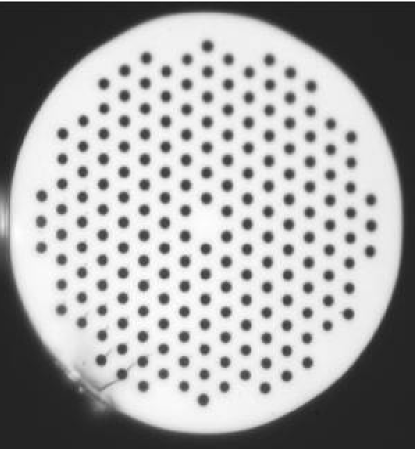
Figure 1: Optical micrograph of a silica-based PCF with a pitch $\Lambda$ of order 10 microns and $d/\Lambda\sim 0.5$. Courtesy of Crystal Fibre A/S, www.crystal-fibre.com.

Photonic crystal fibres (PCF) are a special class of optical fibres where a remarkable dielectric topology facilitates unique optical properties. Guiding of light is accomplished by a highly regular array of air holes running along the full length of the fibre, see Fig. 1. In their simplest form the fibres employ a single dielectric base material (with dielectric function $\varepsilon_{b}=n_{b}^{2}$) and for the majority of fabricated fibres silica has been the most common choice [1, 2]. This preference has of course been highly motivated by silica’s transparency in the visible to infrared regimes, but has also been strongly driven by the highly matured glass technology used in the fabrication of standard telecommunication fibres. However, a growing interest in fibre optics for other wavelengths and light sources has recently led to a renewed interest in other base materials including chalcogenide glass [3], lead silicate glass [4], telluride glass [5], bismuth glass [6], silver halide [7], teflon [8], and plastics/polymers [9].

The huge theoretical and numerical effort in the PCF community has been important in understanding the dispersion and modal properties, but naturally there has been a clear emphasize on silica-based PCFs. PCFs fabricated from different base materials typically share the same overall geometry with the air holes arranged in a triangular lattice and the core defect being formed by the removal of a single air-hole. However, it is not yet fully clarified how the established understanding may be transferred to the development of PCFs made from other base materials. To put it simple; PCFs made from different base materials share the same topology, but to which extend do they also have optical characteristics in common?

When addressing this question it is important to realize that the otherwise very useful concept of scale-invariance of Maxwell’s equations [10] is of little direct use in this particular context. Since PCFs made from different base materials do not relate to each other by a linear scaling of the dielectric function, $\varepsilon({\boldsymbol{r}})\nrightarrow s^{2}\varepsilon({\boldsymbol{r}})$, scale invariance cannot be applied directly to generalize the results for e.g. silica to other base materials. Electro-magnetic perturbation theory is of course one possible route allowing us to take small changes of the base-material refractive index into account, but in this paper we will discuss and elaborate on an alternative approach which was put forward recently [11].

As a starting point we take the classical description based on Maxwell’s equations, which for linear dielectric materials simplify to the following vectorial wave-equation for the electrical field [10]

$${\boldsymbol{\nabla}}\times{\boldsymbol{\nabla}}\times{\boldsymbol{E}}({\boldsymbol{r}})=\varepsilon({\boldsymbol{r}})\frac{\omega^{2}}{c^{2}}\>{\boldsymbol{E}}({\boldsymbol{r}}).$$ (1)

Here, $\varepsilon$ is the dielectric function which in our case takes the material values of either air or the base material. For a fibre geometry with $r_{\parallel}$ along the fibre axis we have $\varepsilon({\boldsymbol{r}})=\varepsilon({\boldsymbol{r}}_{\perp})$ and as usual we search for solutions of the plane-wave form $e^{i(\beta r_{\parallel}-\omega t)}$ with the goal of calculating the dispersion $\omega(\beta)$ relation.

2 Short-wavelength approximations

Today, several approaches are available for solving Eq. (1) numerically, including plane-wave, multi-pole, and finite-element methods [12, 13, 14]. Such methods will typically be preferred in cases where highly quantitative correct results are called for. However, numerical studies do not always shine much light on the physics behind so here we will take advantage of several approximations which allow for analytical results in the short-wavelength limit $\lambda\ll\Lambda$. The key observation allowing for the approximations is that typically the base material has a dielectric function exceeding that of air significantly, $\varepsilon_{b}\gg 1$. In that case it is well-known that the short-wavelength regime is characterized by having the majority of the electrical field residing in the high-index base material while the fraction of electrical field in the air holes is vanishing.

The, at first sight very crude, approximation is simply to neglect the small fraction of electrical power residing in the air-hole regions. Mathematically the approximation is implemented by imposing the boundary condition that ${\boldsymbol{E}}$ is zero at the interfaces $\partial\Omega$ to air. Since the displacement field ${\boldsymbol{D}}=\varepsilon{\boldsymbol{E}}$ is divergence free we have $0=\varepsilon{\boldsymbol{\nabla}}\cdot{\boldsymbol{E}}+{\boldsymbol{E}}\cdot{\boldsymbol{\nabla}}\varepsilon\approx\varepsilon{\boldsymbol{\nabla}}\cdot{\boldsymbol{E}}$ and the wave equation (1) now reduces to

$$-{\boldsymbol{\nabla}}^{2}{\boldsymbol{E}}({\boldsymbol{r}})\approx\varepsilon_{b}\frac{\omega^{2}}{c^{2}}\>{\boldsymbol{E}}({\boldsymbol{r}}),\quad{\boldsymbol{E}}({\boldsymbol{r}})\Big{|}_{{\boldsymbol{r}}\in\partial\Omega}=0,$$ (2)

and since solutions are of the plane-wave form $e^{i(\beta r_{\parallel}-\omega t)}$ along the fiber axis we get

$$-{\boldsymbol{\nabla}}_{\perp}^{2}{\boldsymbol{E}}({\boldsymbol{r}}_{\perp})+\beta^{2}{\boldsymbol{E}}({\boldsymbol{r}}_{\perp})\approx\varepsilon_{b}\frac{\omega^{2}}{c^{2}}\>{\boldsymbol{E}}({\boldsymbol{r}}_{\perp}),\quad{\boldsymbol{E}}({\boldsymbol{r}}_{\perp})\Big{|}_{{\boldsymbol{r}}_{\perp}\in\partial\Omega}=0,$$ (3)

where ${\boldsymbol{\nabla}}_{\perp}^{2}$ is two-dimensional Laplacian in the transverse plane. The essentially scalar nature of this equation makes the problem look somewhat similar to the more traditional scalar approximation

$${\boldsymbol{\nabla}}_{\perp}^{2}\Psi({\boldsymbol{r}}_{\perp})+\varepsilon({\boldsymbol{r}}_{\perp})\frac{\omega^{2}}{c^{2}}\>\Psi({\boldsymbol{r}}_{\perp})\approx\beta^{2}\>\Psi({\boldsymbol{r}}_{\perp}),$$ (4)

that has been applied successfully to PCFs in the short-wavelength regime [15]. However, while that approach took the field and the dielectric function in the air holes into account we shall here solve Eq. (3) with the boundary condition that ${\boldsymbol{E}}$ is zero at the interfaces to air. We note that this of course is fully equivalent to solving Eq. (4) with the boundary condition that $\Psi$ is zero at the interfaces to air. Obviously, the scalar problem posed by Eq. (3) is separable and formally we have that

$$\omega=\sqrt{\Omega_{\perp}^{2}+\Omega_{\parallel}^{2}}=\sqrt{\Omega_{\perp}^{2}+\left(c\beta/n_{b}\right)^{2}}$$ (5)

where $\Omega_{\parallel}=c\beta/n_{b}$ is the frequency associated with the longitudinal plane-wave propagation with a linear dispersion relation (i.e. $\Omega_{\parallel}\propto\beta$) and $\Omega_{\perp}$ is the frequency associated with the transverse confinement/localization. At this point we already note how an arbitrary base-material refractive index $n_{b}$ enters in the frequency associated with the longitudinal plane-wave propagation. This is solely possible because we have a Dirichlet boundary condition in Eq. (3) which does not depend on the refractive index of the base material.

3 The Schrödinger equation eigenvalue problem

In the following we rewrite Eq. (5) as

$$\omega=\frac{c}{n_{b}}\sqrt{\gamma^{2}\Lambda^{-2}+\beta^{2}}$$ (6)

where now $\gamma$ is a dimensionless number characterizing the confinement/localization. It is of purely geometrical origin and thus only depends on the normalized air-hole diameter $d/\Lambda$. From Eq. (3) it follows that $\gamma$ is an eigenvalue governed by a scalar two-dimensional Schrödinger equation

$$-\Lambda^{2}{\boldsymbol{\nabla}}_{\perp}^{2}\psi({\boldsymbol{r}}_{\perp})=\gamma^{2}\psi({\boldsymbol{r}}_{\perp}),\quad\psi({\boldsymbol{r}}_{\perp})\Big{|}_{{\boldsymbol{r}}_{\perp}\in\partial\Omega}=0.$$ (7)

The same equation was recently studied in work on anti-dot lattices in a two-dimensional electron gas [16] and there will be many similarities between such quantum mechanical electron systems and the present electromagnetic problem. In the language of quantum mechanics the wavefunction $\psi$ is subject to hard-wall boundary conditions corresponding to an infinite potential barrier in the air-hole regions. The task of calculating the optical dispersion properties has now reduced to solving the scalar two-dimensional Schrödinger-like eigenvalue problem posed by Eq. (7). The strength is obviously that Eq. (7) is material independent and thus we may in principle solve it once and for all to get the geometry dependence of $\gamma$ and thereby the optical dispersion of the PCF. In the following we solve Eq. (7) for different classes of modes and compare approximate results to corresponding numerically exact finite-element solutions.

3.1 The fundamental space-filling mode

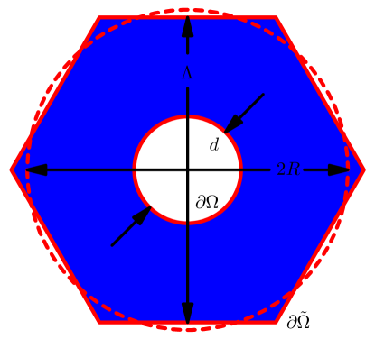
Figure 3: The hexagonal Wigner–Seitz unit cell of the periodic triangular lattice with lattice constant/pitch $\Lambda$. The dashed line indicates the annular region which has the same area as the doubly-connected domain of hexagonal outer shape. Dirichlet and Neumann boundary conditions apply to the inner and outer boundaries $\partial\Omega$ and $\partial\tilde{\Omega}$, respectively.

The fundamental space-filling mode is a key concept in understanding the light guiding properties of PCFs. It is the fundamental de-localized mode of Eq. (7) in an infinite periodic structure and the corresponding mode index corresponds to an effective material index of the artificial periodic photonic crystal lattice. In the language of band diagrams and Brillouin zones it is defined in the $\Gamma$-point where Bloch’s theorem is particular simple; as illustrated in Fig. 3 the wave function is subject to a simple Neumann boundary condition on the edge $\partial\tilde{\Omega}$ of the Wigner–Seitz cell, i.e.

$$-\Lambda^{2}{\boldsymbol{\nabla}}_{\perp}^{2}\psi({\boldsymbol{r}}_{\perp})=\gamma_{\rm cl}^{2}\psi({\boldsymbol{r}}_{\perp}),\quad\psi({\boldsymbol{r}}_{\perp})\Big{|}_{{\boldsymbol{r}}_{\perp}\in\partial\Omega}={\boldsymbol{n}}\cdot{\boldsymbol{\nabla}}\psi({\boldsymbol{r}}_{\perp})\Big{|}_{{\boldsymbol{r}}_{\perp}\in\partial\tilde{\Omega}}=0,$$ (8)

where ${\boldsymbol{n}}$ is a unit vector normal to the boundary $\partial\tilde{\Omega}$. We thus have to solve an eigenvalue problem on a doubly-connected domain. By a conformal mapping, leaving the Laplacian and the boundary conditions invariant, one may in principle transform the hexagonal shape with the circular hole of diameter $d$ into a simple annular region of inner diameter $d$ and outer diameter $2R$ [17] leaving us with an eigenvalue problem in the radial coordinate. Finding the exact conformal mapping may be a complicated task so here we simply use the approximate mapping with

$$R=\Lambda\sqrt{\frac{\sqrt{3}}{2\pi}}\simeq 0.53\,\Lambda$$ (9)

which serves to conserve the area of the Wigner–Seitz unit cell. Neglecting any small changes to the eigenvalue equation caused during the mapping we get the following eigenvalue equation in the radial coordinate,

$$-\Lambda^{2}(\partial_{r}^{2}+r^{-1}\partial_{r})\psi(r)\approx\gamma_{\rm cl}^{2}\psi(r),\quad\psi(d/2)=\psi^{\prime}(R)=0.$$ (10)

The solution is given by a linear combination of the Bessel functions $J_{0}$ and $Y_{0}$ and the eigenvalue is determined by the roots of the following expression

$$J_{1}\left(\frac{3^{\frac{1}{4}}}{{\sqrt{2\,\pi}}}\gamma_{\rm cl}\right)Y_{0}\left(\frac{1}{2}\frac{d}{\Lambda}\gamma_{\rm cl}\right)=J_{0}\left(\frac{1}{2}\frac{d}{\Lambda}\gamma_{\rm cl}\right)Y_{1}\left(\frac{3^{\frac{1}{4}}\,}{{\sqrt{2\,\pi}}}\gamma_{\rm cl}\right).$$ (11)

In general the equation cannot be solved exactly except for at the point

$$\left\{\frac{d}{\Lambda},\gamma_{\rm cl}^{2}\right\}=\left\{2\frac{3^{1/4}}{\sqrt{2\pi}}\>\frac{\alpha_{0,1}}{\alpha_{1,1}},\frac{2\pi}{3^{1/2}}\>\alpha_{1,1}^{2}\right\}\simeq\left\{0.66,53.26\right\},$$ (12)

as is easily verified by insertion and using that $\alpha_{n,m}$ is the $m$th zero of the $n$th Bessel function, i.e. $J_{n}(\alpha_{n,m})=0$. In particular we have that $\alpha_{0,1}\simeq 2.405$ and $\alpha_{1,1}\simeq 3.8317$. However, expanding the left and right-hand sides of Eq. (12) around this point to first order in both $\gamma_{\rm cl}$ and $d/\Lambda$ we get an equation from which we may isolate $\gamma_{\rm cl}$ yielding an approximate analytical solution of the form

$$\gamma_{\rm cl}^{2}\simeq\left({\cal C}_{1}+\frac{{\cal C}_{2}}{{\cal C}_{3}-d/\Lambda}\right)^{2}.$$ (13)

The coefficients are given by expressions involving Bessel functions $Y_{0}$ and $Y_{1}$ evaluated at $\alpha_{0,1}$ and $\alpha_{1,1}$, see Appendix, but for simplicity we here only give the corresponding numerical values of these expressions; ${\cal C}_{1}\simeq-0.2326$, ${\cal C}_{2}\simeq 2.7040$, and ${\cal C}_{3}\simeq 1.0181$.

3.2 Core-defect modes

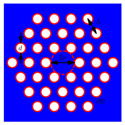
Figure 2: The topology of a PCF formed by omitting an air hole of diameter $d$ in a triangular lattice of air holes with pitch $\Lambda$. Dirichlet boundary conditions are applied to the boundary $\partial\Omega$ indicated by red solid lines. The red dashed line indicates twice an effective core radius $\rho=\Lambda-d/2$.

While the fundamental space-filling mode, discussed above, is a de-localized mode it is also possible to have strongly localized states, especially in the presence of defects such as one formed by removing an air hole from the otherwise periodic lattice of air holes, see figures 1 and 2. In this way light can be guided along the defect thus forming the core of the fibre. The requirement for corralling the light is of course that the core-defect mode has an eigenvalue $\gamma_{c,1}^{2}$ not exceeding the corresponding eigenvalue $\gamma_{\rm cl}^{2}$ of the surrounding photonic crystal cladding. To put it slightly different the defect in the air-hole lattice effectively corresponds to a potential well of depth $\gamma_{\rm cl}^{2}$ and a radius roughly given by $\rho=\Lambda-d/2$, see Fig. 2.

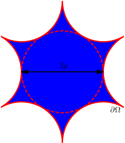
Figure 4: Zoom in on the core-defect in the extreme limit of $d/\Lambda=1$. A Dirichlet boundary condition applies to the boundary $\partial\Omega$ and the dashed circle indicates the approximate core radius $\rho=\Lambda-d/2$.

In order to calculate the fundamental core-defect mode we first note that in the limit of $d/\Lambda$ approaching 1, the problem can be approximated with that of a two-dimensional spherical infinite potential well with radius $\rho=\Lambda-d/2$, see Fig. 4. For this problem the lowest eigenvalue is

$$\gamma_{c,1}^{2}\sim\left(\frac{\Lambda}{\rho}\right)^{2}\alpha_{0,1}^{2}=\frac{\alpha_{0,1}^{2}}{\left(1-\frac{1}{2}\frac{d}{\Lambda}\right)^{2}}.$$ (14)

Although this expression yields the correct scaling with $d/\Lambda$, the approximation obviously breaks down for small values of $d/\Lambda$. In that limit we follow the ideas of Glazman et al. [18], who studied quantum conductance through narrow constrictions. The effective one-dimensional energy barrier for transmission through the constriction of width $\Lambda-d$ between two neighbouring holes has a maximum value of $\pi^{2}$ in the limit where $d$ goes to zero. We thus approximate the $d/\Lambda\rightarrow 0$ problem with that of a two-dimensional spherical potential well of height $\pi^{2}$ and radius $\Lambda$,

$$-\Lambda^{2}(\partial_{r}^{2}+r^{-1}\partial_{r})\psi(r)+\pi^{2}\Theta(r-\Lambda)\psi(r)=\tilde{\gamma}_{c,1}^{2}\psi(r),$$ (15)

where $\Theta(x)$ is the Heaviside step function which is zero for $x<0$ and unity for $x>0$. The lowest eigenvalue $\tilde{\gamma}_{c,1}^{2}$ for this problem is the first root of the following equation

$$\tilde{\gamma}_{c,1}\frac{J_{1}(\tilde{\gamma}_{c,1})}{J_{0}(\tilde{\gamma}_{c,1})}=\sqrt{\pi^{2}-\tilde{\gamma}_{c,1}^{2}}\frac{K_{1}\left(\sqrt{\pi^{2}-\tilde{\gamma}_{c,1}^{2}}\>\right)}{K_{0}\left(\sqrt{\pi^{2}-\tilde{\gamma}_{c,1}^{2}}\>\right)}.$$ (16)

In the case where the potential $\pi^{2}$ is replaced by an infinite potential the first root is given by $\alpha_{0,1}^{2}$. Lowering the confinement potential obviously shifts down the eigenvalue and in the present case the eigenvalue is roughly $\tilde{\gamma}_{c,1}^{2}\sim\pi$. In fact, expanding the equation to first order in $\tilde{\gamma}_{c,1}$ around e.g. $\sqrt{\pi}$ we get a straight forward, but long, expression with the numerical value $\tilde{\gamma}_{c,1}^{2}\simeq 3.221$ which is in excellent agreement with a numerical solution of the equation. Correcting for the low-$d/\Lambda$ behaviour we thus finally get

$$\gamma_{c,1}^{2}\simeq\tilde{\gamma}_{c,1}^{2}+\left\{1-\lim_{d/\Lambda\rightarrow 0}\right\}\frac{\alpha_{0,1}^{2}}{\left(1-\frac{1}{2}\frac{d}{\Lambda}\right)^{2}}=\tilde{\gamma}_{c,1}^{2}+\frac{\left(4-\frac{d}{\Lambda}\right)\frac{d}{\Lambda}}{\left(2-\frac{d}{\Lambda}\right)^{2}}\>\alpha_{0,1}^{2}.$$ (17)

For the first high-order mode we may apply a very similar analysis. This mode has a finite angular momentum of $\pm 1$ with a radial $J_{1}$ solution yielding

$$\gamma_{c,2}^{2}\simeq\tilde{\gamma}_{c,2}^{2}+\frac{\left(4-\frac{d}{\Lambda}\right)\frac{d}{\Lambda}}{\left(2-\frac{d}{\Lambda}\right)^{2}}\>\alpha_{1,1}^{2}.$$ (18)

Here, $\tilde{\gamma}_{c,2}^{2}\simeq 7.673$ is the second eigenvalue of the two-dimensional spherical potential well of height $\pi^{2}$ and radius $\Lambda$. Again, it can be found from an equation very similar to Eq. (16).

3.3 Two-dimensional finite-element solutions

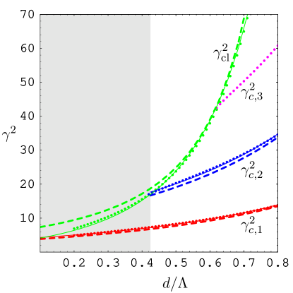
Figure 5: Geometrical eigenvalues $\gamma^{2}$ versus normalized air-hole diameter $d/\Lambda$. The data points are results of finite-element simulations while the corresponding dashed lines are the approximate results in Eqs. (13), (17), and (18). The thin solid lines shows the numerical fits listed in Eqs. (19a), (19b), and (19c). Note how only a single core-defect mode is supported in the shaded region, $d/\Lambda\lesssim 0.42$.

Above we have solved the geometrical eigenvalue problem analytically by means of various approximations. In this section we compare the quality of these results by direct comparison to a numerically exact solution of the two-dimensional eigenvalue problem. The developments in computational physics and engineering have turned numerical solutions of partial differential equations in the direction of a standard task. Here, we employ a finite-element approach[19] to numerically solve Eq. (7) and calculate $\gamma^{2}$ versus $d/\Lambda$. We employ an adaptive mesh algorithm to provide efficient convergence. For cladding mode we implement Eq. (8) directly while for the defect modes we solve Eq. (7) on a finite domain of approximate size $10\Lambda\times 10\Lambda$ with the defect located in the center of the domain. For $d/\Lambda$ down to around 0.1 we have found this to sufficient to adequate convergence for the strongly localized defect states, thus avoiding strong proximity from the domain-edge boundary condition which for simplicity has been of the Dirichlet type. Figure 5 summarizes our numerical results for the first cladding mode $\gamma_{\rm cl}^{2}$ as well for the two first core-defect modes $\gamma_{c,1}^{2}$ and $\gamma_{c,2}^{2}$. The dashed lines indicate the corresponding approximate expressions in Eqs. (13), (17), and (18) obtained by analytical means. As seen the qualitative agreement is excellent, but in order to facilitate also quantitative applications of the results we also include the results of numerical least-square error fits below. The thin solid lines show the expressions

$$\gamma_{c,1}^{2} \simeq 3.666+\frac{\left(4-\frac{d}{\Lambda}\right)\frac{d}{\Lambda}}{\left(2-\frac{d}{\Lambda}\right)^{2}}\>\alpha_{0,1}^{2},$$ (19a)

$$\gamma_{c,2}^{2} \simeq 8.691+\frac{\left(4-\frac{d}{\Lambda}\right)\frac{d}{\Lambda}}{\left(2-\frac{d}{\Lambda}\right)^{2}}\>\alpha_{1,1}^{2},$$ (19b)

$$\gamma_{cl}^{2} \simeq\left(-2.82476+\frac{5.23695}{1.17908-d/\Lambda}\right)^{2},$$ (19c)

which match the numerical data within a relative error of less than $2\%$ around the most important cut-off region $d/\Lambda\sim 0.42$.

4 Derived fiber optical parameters

With Eq. (6) at hand we have now provided a unified theory of the dispersion relation in the short-wavelength regime for PCFs with arbitrary base materials and Eq. (6) illustrates how geometrical confinement modifies the linear free-space dispersion relation.

In fibre optics it is common to express the dispersion properties in terms of the effective index $n_{\rm eff}=c\beta/\omega$ versus the free-space wavelength $\lambda=c2\pi/\omega$. From Eq. (6) it follows straightforwardly that

$$n_{\rm eff}=n_{b}\sqrt{1-\frac{\gamma^{2}}{4\pi^{2}n_{b}^{2}}\left(\frac{\lambda}{\Lambda}\right)^{2}}$$ (20)

which obviously is in qualitative agreement with the accepted view that $n_{\rm eff}$ increases monotonously with decreasing wavelength and approaches $n_{b}$ in the asymptotic short-wavelength limit as reported for e.g. silica-based PCFs [2]. Similarly, the group-velocity $v_{g}=\partial\omega/\partial\beta$ becomes

$$v_{g}=\frac{c}{n_{b}}\sqrt{1-\frac{\gamma_{c,1}^{2}}{4\pi^{2}n_{b}^{2}}\left(\frac{\lambda}{\Lambda}\right)^{2}}$$ (21)

while the phase velocity $v_{p}=\omega/\beta$ becomes

$$v_{p}=\frac{c}{n_{b}}\frac{1}{\sqrt{1-\frac{\gamma_{c,1}^{2}}{4\pi^{2}n_{b}^{2}}\left(\frac{\lambda}{\Lambda}\right)^{2}}}.$$ (22)

The group-velocity dispersion is most often quantified by the wave-guide dispersion parameter $D_{\rm wg}=\partial(1/v_{g})/\partial\lambda$ which becomes

$$D_{\rm wg}=\frac{1}{c\Lambda}\frac{\gamma_{c,1}^{2}}{4\pi^{2}n_{b}}\left[1-\frac{\gamma_{c,1}^{2}}{4\pi^{2}n_{b}^{2}}\left(\frac{\lambda}{\Lambda}\right)^{2}\right]^{-3/2},$$ (23)

where any possible material dispersion $n_{b}(\lambda)$ has been neglected. We note that since $D_{\rm wg}>0$ the geometry of the air-hole lattice always causes a positive wave-guide dispersion parameter. Large-mode area PCFs belong to the regime with $\lambda\ll\Lambda$ were we predict the following general magnitude of the wave-guide dispersion of a large-mode area PCF

$$\lim_{\lambda\ll\Lambda}D_{\rm wg}=\frac{1}{c\Lambda}\frac{\gamma_{c,1}^{2}}{4\pi^{2}n_{b}}.$$ (24)

Finally, the recently suggested parameter $V_{\rm PCF}=\Lambda\sqrt{\beta_{\rm cl}^{2}-\beta_{c,1}^{2}}$ [20] can be shown to be a purely geometrically defined parameter in the large-mode area limit. From Eq. (6) it follows straightforwardly that

$$\lim_{\lambda\ll\Lambda}V_{\rm PCF}=\sqrt{\gamma_{\rm cl}^{2}-\gamma_{c,1}^{2}}.$$ (25)

This implies that the endlessly single-mode property [2, 21, 20, 22] is a wave phenomena independent of the base material refractive index of purely geometrical origin. Higher-order modes are only supported for $d/\Lambda\gtrsim 0.42$, as seen in Fig. 5, for which $V_{\rm PCF}\gtrsim\pi$ [20].

5 Comparison to fully-vectorial plane-wave simulations

In the previous sections substantial analytical progress was made, but we still remain to address the question to which extend the basic assumption behind Eq. (3) holds except that it becomes exact for the fundamental modes as $\lambda/\Lambda$ approaches zero. In Fig. 6 we compare the analytical results for the effective index in Eq. (20) to results obtained by fully-vectorial plane-wave simulations [12] of Eq. (1). For the fundamental space-filling mode we have employed a basis of $2^{6}\times 2^{6}$ plane waves while for the core-defect modes we have employed a super-cell configuration of size $10\Lambda\times 10\Lambda$ in the case of $d/\Lambda=0.4$.

Panel (a) shows results for the fundamental space-filling mode for various values of the base refractive index. As clearly seen the theory agrees excellently in the short-wavelength limit while pronounced deviations occur as the wavelength increases and the field penetrates deeper into the air hole regions and also vectorial effects become important as reported in [15]. Similar conclusion applies to the corresponding results in panel (c) for the fundamental core-defect mode. While $d/\Lambda=0.4$ is a case of particular technological interest because of its endlessly single-mode property we would like to emphasize that equivalent agreement is found for other values of $d/\Lambda$ (results not shown). However, since the success of the approximation in Eq. (3) really is that $\lambda/n_{b}\ll 2\rho=2\Lambda-d$ and $\lambda/n_{b}\ll\Lambda-d$ for the core and cladding results, respectively, there will of course be a small $d$-dependence. However, this also indicates that the agreement will increase with an increasing refractive index $n_{b}$ of the base material as has also been observed for even higher values of $n_{b}$ than those studied in Fig. 6 (results not shown).

6 Discussion and conclusion

It is today more than 10 years ago that the PCF was invented by Russell and co-workers [1] and there is a still growing community of researchers directing their efforts toward fabrication and experimental studies of silica-based PCFs as well as quantitative modelling of the optical properties. At the same time the community is obviously facing the challenges and opportunities of new exciting fiber materials. PCFs made from different base materials share the same topology so it seems quite natural to assume that they also have at least some basic optical properties in common. Let’s return to the question posed in the introduction: to which extend do PCFs made from different materials have optical characteristics in common? The present work do to some extend address this question. Most importantly we illustrate how the waveguide dispersion originates from the geometrical transverse confinement/localization of the mode and how the endlessly single-mode property arises as a sole consequence of the geometry which acts as a modal sieve. In particular we have shown how PCFs are endlessly single-mode for $d/\Lambda\lesssim 0.42$ irrespectively of the base material an analytical expression for the wave-guide dispersion parameter applicable to large-mode area fibres.

For small-core PCFs our theory provides qualitative correct results though more quantitative insight still calls for fully vectorial simulations, see e.g. [23]. However, for large-mode area PCFs our expressions not only gives qualitative insight, but also quantitative correct expressions which may be used in straightforward design of large-mode area PCFs with special properties with respect to the group-velocity dispersion and the susceptibility of the fundamental mode with respect to longitudinal non-uniformities [24].

Appendix A Taylor expansion of Eq. (11)

Taylor expanding the left and right-hand sides of Eq. (11) around the point

$$\left\{d_{0}\>,\>\gamma_{0}\right\}\equiv\left\{2\frac{3^{1/4}}{\sqrt{2\pi}}\>\frac{\alpha_{0,1}}{\alpha_{1,1}}\>\Lambda\>,\>\sqrt{\frac{2\pi}{3^{1/2}}}\>\alpha_{1,1}\right\}$$ (26)

to first order in both $\gamma_{\rm cl}$ and $d/\Lambda$ we get

$$0= \left(\frac{d-d_{0}}{d_{0}}\right)+\frac{Y_{1}^{2}(\alpha_{1,1})-Y_{0}^{2}(\alpha_{0,1})}{Y_{1}^{2}(\alpha_{1,1})}\left(\frac{\gamma_{\rm cl}-\gamma_{0}}{\gamma_{0}}\right)$$

$$+\frac{Y_{1}(\alpha_{0,1})}{Y_{0}(\alpha_{0,1})}\frac{d_{0}}{\Lambda}\left(\frac{d-d_{0}}{d_{0}}\right)\left(\gamma_{\rm cl}-\gamma_{0}\right)$$

$$+{\cal O}\left([d-d_{0}]^{2}\right)+{\cal O}\left([\gamma_{\rm cl}-\gamma_{0}]^{2}\right).$$ (27)

Next, solving for $\gamma_{\rm cl}$ we may write the result in the form of Eq. (13) with

$${\cal C}_{1} =\gamma_{0}-\frac{Y_{0}(\alpha_{0,1})}{Y_{1}(\alpha_{0,1})}\left(\frac{d_{0}}{\Lambda}\right)^{-1},$$ (28a)

$${\cal C}_{2} =\frac{Y_{0}^{4}(\alpha_{0,1})-Y_{0}^{2}(\alpha_{0,1})\,Y_{1}^{2}(\alpha_{1,1})}{\gamma_{0}\,{Y_{1}^{2}(\alpha_{0,1})}\,{Y_{1}^{2}(\alpha_{1,1})}}\left(\frac{d_{0}}{\Lambda}\right)^{-1},$$ (28b)

$${\cal C}_{3} =\frac{{Y_{0}^{3}(\alpha_{0,1})}-Y_{0}(\alpha_{0,1})\,{Y_{1}^{2}(\alpha_{1,1})}}{\gamma_{0}\,Y_{1}(\alpha_{0,1})\,{Y_{1}^{2}(\alpha_{1,1})}}+\frac{d_{0}}{\Lambda},$$ (28c)

which have the numerical values listed in the paragraph below Eq. (13).

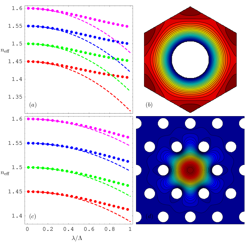
Figure 6: Effective index versus normalized wavelength $\lambda/\Lambda$ for the fundamental space-filling mode (a) and the fundamental core-defect mode (c) for a PCF with $d/\Lambda=0.4$ with a base material refractive index $n_{b}$ varying from 1.45 to 1.6 in steps of 0.05 from below. The data points are the results of a vectorial plane-wave simulation of Eq. (1) while the dashed lines show the corresponding results based on Eq. (20) with Eqs. (19a) and (19c) for geometrical eigenvalues $\gamma_{\rm cl}^{2}$ and $\gamma_{c,1}^{2}$. Panels (b) and (d) show the corresponding eigenfunctions $\psi$.

REFERENCES

- [1] J. C. Knight, T. A. Birks, P. S. J. Russell, and D. M. Atkin, “All-silica single-mode optical fiber with photonic crystal cladding”, Opt. Lett. 21 1547–1549 (1996).
- [2] T. A. Birks, J. C. Knight, and P. S. J. Russell, “Endlessly single mode photonic crystal fibre”, Opt. Lett. 22 961–963 (1997).
- [3] T. M. Monro, Y. D. West, D. W. Hewak, N. G. R. Broderick, and D. J. Richardson, “Chalcogenide holey fibres”, Electron. Lett. 36 1998–2000 (2000).
- [4] V. V. R. K. Kumar, A. K. George, W. H. Reeves, J. C. Knight, P. S. J. Russell, F. G. Omenetto, and A. J. Taylor, “Extruded soft glass photonic crystal fiber for ultrabroad supercontinuum generation”, Opt. Express 10 1520–1525 (2002).
- [5] V. V. R. K. Kumar, A. K. George, J. C. Knight, and P. S. J. Russell, “Tellurite photonic crystal fiber”, Opt. Express 11 2641–2645 (2003).
- [6] H. Ebendorff-Heidepriem, P. Petropoulos, S. Asimakis, V. Finazzi, R. C. Moore, K. Frampton, F. Koizumi, D. J. Richardson, and T. M. Monro, “Bismuth glass holey fibers with high nonlinearity”, Opt. Express 12 5082–5087 (2004).
- [7] E. Rave, P. Ephrat, M. Goldberg, E. Kedmi, and A. Katzir, “Silver halide photonic crystal fibers for the middle infrared”, Appl. Opt. 43 2236–2241 (2004).
- [8] M. Goto, A. Quema, H. Takahashi, S. Ono, and N. Sarukura, “Teflon photonic crystal fiber as terahertz waveguide”, Jap. J. Appl. Phys. 43 L317–L319 (2004).
- [9] M. A. van Eijkelenborg, M. C. J. Large, A. Argyros, J. Zagari, S. Manos, N. A. Issa, I. Bassett, S. Fleming, R. C. McPhedran, C. M. de Sterke, and N. A. P. Nicorovici, “Microstructured polymer optical fibre”, Opt. Express 9 319–327 (2001).
- [10] J. D. Joannopoulos, R. D. Meade, and J. N. Winn, Photonic crystals: molding the flow of light (Princeton University Press, Princeton, 1995).
- [11] N. A. Mortensen, “Semianalytical approach to short-wavelength dispersion and modal properties of photonic crystal fibers”, Opt. Lett. 30 1455 – 1457 (2005).
- [12] S. G. Johnson and J. D. Joannopoulos, “Block-iterative frequency-domain methods for Maxwell’s equations in a planewave basis”, Opt. Express 8 173–190 (2001).
- [13] B. T. Kuhlmey, T. P. White, G. Renversez, D. Maynstre, L. C. Botton, C. M. de Sterke, and R. C. McPhedran, “Multipole method for microstructured optical fibers. II. Implementation and results”, J. Opt. Soc. Am. B 19 2331–2340 (2002).
- [14] K. Saitoh and M. Koshiba, “Full-vectorial imaginary-distance beam propagation method based on finite element scheme: Application to photonic crystal fibers”, IEEE J. Quantum Electron. 38 927–933 (2002).
- [15] J. Riishede, N. A. Mortensen, and J. Lægsgaard, “A poor man’s approach to modelling of microstructured optical fibers”, J. Opt. A: Pure. Appl. Opt. 5 534 (2003).
- [16] C. Flindt, N. A. Mortensen, and A. P. Jauho, “Quantum computing via defect states in two-dimensional antidot lattices”, Nano Lett. 5 2515 – 2518 (2005).
- [17] P. A. Laura, E. Romanelli, and M. J. Maurizi, “On the analysis of waveguides of double-connected cross-section by the method of conformal mapping”, J. Sound Vibr. 20 27–38 (1972).
- [18] L. I. Glazman, G. K. Lesovik, D. E. Khmelnitskii, and R. I. Shekter, “Reflectionsless quantum transport and fundamental ballistic-resistance steps in microscopic constrictions”, JETP Lett. 48 238–241 (1988).
- [19] Femlab, http://www.comsol.com.
- [20] N. A. Mortensen, J. R. Folkenberg, M. D. Nielsen, and K. P. Hansen, “Modal cut-off and the –parameter in photonic crystal fibers”, Opt. Lett. 28 1879–1881 (2003).
- [21] N. A. Mortensen, “Effective area of photonic crystal fibers”, Opt. Express 10 341–348 (2002).
- [22] K. Saitoh, Y. Tsuchida, M. Koshiba, and N. A. Mortensen, “Endlessly single-mode holey fibers: the influence of core design”, Opt. Express 13 10833 – 10839 (2005).
- [23] K. Saitoh, M. Koshiba, and N. A. Mortensen, “Nonlinear photonic crystal fibres: pushing the zero-dispersion toward the visible”, Special issue on nanophotonics to appear in New J. Phys. (2006). http://arxiv.org/physics/0608142
- [24] N. A. Mortensen and J. R. Folkenberg, “Low-loss criterion and effective area considerations for photonic crystal fibers”, J. Opt. A: Pure Appl. Opt. 5 163–167 (2003).