Numerical Study of Nearly Singular Solutions of the 3-D Incompressible Euler Equations

Abstract

In this paper, we perform a careful numerical study of nearly singular solutions of the 3D incompressible Euler equations with smooth initial data. We consider the interaction of two perturbed antiparallel vortex tubes which was previously investigated by Kerr in [14, 17]. In our numerical study, we use both the pseudo-spectral method with the 2/3 dealiasing rule and the pseudo-spectral method with a high order Fourier smoothing. Moreover, we perform a careful resolution study with grid points as large as $1536\times 1024\times 3072$ to demonstrate the convergence of both numerical methods. Our computational results show that the maximum vorticity does not grow faster than doubly exponential in time while the velocity field remains bounded up to $T=19$, beyond the singularity time $T=18.7$ reported by Kerr in [14, 17]. The local geometric regularity of vortex lines near the region of maximum vorticity seems to play an important role in depleting the nonlinear vortex stretching dynamically.

1 Introduction

The question of whether the solution of the 3D incompressible Euler equations can develop a finite time singularity from a smooth initial condition is one of the most challenging problems. A major difficulty in obtaining the global regularity of the 3D Euler equations is due to the presence of the vortex stretching, which is formally quadratic in vorticity. There have been many computational efforts in searching for finite time singularities of the 3D Euler and Navier-Stokes equations, see e.g. [5, 21, 18, 12, 22, 14, 4, 2, 10, 20, 11, 17]. Of particular interest is the numerical study of the interaction of two perturbed antiparallel vortex tubes by Kerr [14, 17], in which a finite time blowup of the 3D Euler equations was reported. There has been a lot of interests in studying the interaction of two perturbed antiparallel vortex tubes in the late eighties and early nineties because of the vortex reconnection phenomena observed for the Navier-Stokes equations. While most studies indicated only exponential growth in the maximum vorticity [21, 1, 3, 18, 19, 22], the work of Kerr and Hussain in [18] suggested a finite time blow-up in the infinite Reynolds number limit, which motivated Kerr’s Euler computations mentioned above.

There has been some interesting development in the theoretical understanding of the 3D incompressible Euler equations. It has been shown that the local geometric regularity of vortex lines can play an important role in depleting nonlinear vortex stretching [6, 7, 8, 9]. In particular, the recent results obtained by Deng, Hou, and Yu [8, 9] show that geometric regularity of vortex lines, even in an extremely localized region containing the maximum vorticity, can lead to depletion of nonlinear vortex stretching, thus avoiding finite time singularity formation of the 3D Euler equations.

In a recent paper [13], we have performed well-resolved computations of the 3D incompressible Euler equations using the same initial condition as the one used by Kerr in [14]. In our computations, we use a pseudo-spectral method with a very high order Fourier smoothing to discretise the 3D incompressible Euler equations. The time integration is performed using the classical fourth order Runge-Kutta method with adaptive time stepping to satisfy the CFL stability condition. We use up to $1536\times 1024\times 3072$ space resolution to resolve the nearly singular behavior of the 3D Euler equations. Our computational results demonstrate that the maximum vorticity does not grow faster than doubly exponential in time, up to $t=19$, beyond the singularity time $t=18.7$ predicted by Kerr’s computations [14, 17]. Moreover, we show that the velocity field, the enstrophy, and enstrophy production rate remain bounded throughout the computations. This is in contrast to Kerr’s computations in which the vorticity blows up like $O((T-t)^{-1})$ and the velocity field blows up like $O((T-t)^{-1/2})$. The vortex lines near the region of the maximum vorticity are found to be relatively smooth. With the velocity field being bounded, the non-blowup result of Deng-Hou-Yu [8, 9] can be applied, which implies that there is no blowup of the Euler equations up to $T=19$. The local geometric regularity of the vortex lines near the region of maximum vorticity seems to play an important role in the dynamic depletion of vortex stretching.

The purpose of this paper is to perform a systematic convergence study using two different numerical methods to further validate the computational results obtained in [13]. These two methods are the pseudo-spectral method with the 2/3 dealiasing rule and the pseudo-spectral method with a high order Fourier smoothing. For the 3D Euler equations with periodic boundary conditions, the pseudo-spectral method with the 2/3 dealiasing rule has been used widely in the computational fluid dynamics community. This method has the advantage of removing the aliasing errors completely. On the other hand, when the solution is nearly singular, the decay of the Fourier spectrum is very slow. The abrupt cut-off of the last 1/3 of its Fourier modes could generate significant oscillations due to the Gibbs phenomenon. In our computational study, we find that the pseudo-spectral method with a high order Fourier smoothing can alleviate this difficulty by applying a smooth cut-off at high frequency modes. Moreover, we find that by using a high order smoothing, we can retain more effective Fourier modes than the 2/3 dealiasing rule. This gives a better convergence property. To demonstrate the convergence of both methods, we perform a careful resolution study, both in the physical space and spectrum space. Our extensive convergence study shows that both numerical methods converge to the same solution under mesh refinement. Moreover, we show that the pseudo-spectral method with a high order Fourier smoothing offers better accuracy than the pseudo-spectral method with the 2/3 dealiasing rule.

To understand the differences between our computational results and those obtained by Kerr in [14], we need to make some comparison between Kerr’s computations [14] and our computations. In Kerr’s computations, he used a pseudo-spectral discretization with the 2/3 dealiasing rule in the $x$ and $y$ directions, and a Chebyshev discretization in the $z$-direction with resolution of order $512\times 256\times 192$. In order to prepare the initial data that can be used for the Chebyshev polynomials, Kerr performed some interpolation and used extra filtering. As noted by Kerr [14] (see the top paragraph of page 1729), “An effect of the initial filter upon the vorticity contours at $t=0$ is a long tail in Fig. 2(a)” (see also Figure 2 of this paper). Such “a long tail” is clearly a numerical artifact. In comparison, since we use pseudo-spectral approximations in all three directions, there is no need to perform interpolation or use extra filtering as was done in [14]. Our initial vorticity contours are essentially symmetric (see Figure 1). There is no such “a long tail” in our initial vorticity contours. It seems reasonable to expect that the “long tail” in Kerr’s discrete initial condition could affect his numerical solution at later times.

A more important difference between Kerr’s computations and our computations is the difference between his numerical resolution and ours. From the numerical results presented at $t=15$ and $t=17$ in [14], one can observe noticeable oscillations in the vorticity contours (see Figure 4 of [14] or Figure 22 of this paper). By $t=17$, the two vortex tubes have effectively turned into two thin vortex sheets which roll up at the left edge (see Figures 24 and 25 of this paper). The rolled up portion of the vortex sheet travels backward in time and moves away from the dividing plane (the $x-y$ plane). With only 192 Chebyshev grid points along the $z$-direction in Kerr’s computations, there are not enough grid points to resolve the rolled up portion of the vortex sheet, which is some distance away from the dividing plane. The lack of resolution along the $z$-direction plus the Gibbs phenomenon due to the use of the 2/3 dealiasing rule in the $x$ and $y$ directions may contribute to the oscillations observed in Kerr’s computations. In comparison, we have 3072 grid points along the $z$-direction, which provide about 16 grid points across the singular layer at $t=18$, and about 8 grid points at $t=19$ [13]. It is also worth mentioning that Kerr has only about 100 effective Fourier modes in the $x$ and $y$ directions (see Figure 18 of [14]), while we have about 1300 effective Fourier modes in $|k|$ (see Figures 11 and 12 of this paper). The difference between our resolutions is clearly significant.

It is worth noting that the computations for $t\leq 17$, which Kerr used as the primary evidence for a singularity, is still far from the predicted singularity time, $T=18.7$. With the asymptotic scaling parameter being $T-t=1.7$, the error in the singularity fitting could be of order one. In order to justify the predicted asymptotic behavior of vorticity and velocity blowup, one needs to perform well-resolved computations much closer to the predicted singularity time. As our computations demonstrate, the alleged singularity scaling, $\|\vec{\omega}\|_{\infty}\approx c/(T-t)$, does not persist in time (here $\vec{\omega}$ is vorticity). If we take $T=18.7$, as suggested in [14], the scaling constant, $c$, does not remain constant as $t\rightarrow T$. In fact, we find that $c$ rapidly decays to zero as $t\rightarrow T$ (see Figure 20 of this paper).

The rest of this paper is organized as follows. We describe the set-up of the problem in Section 2. In Section 3, we perform a systematic convergence study of the two numerical methods. We describe our numerical results in detail and compare them with the previous results obtained in [14, 17] in Section 4. Some concluding remarks are made in Section 5.

2 The set-up of the problem

The 3D incompressible Euler equations in the vorticity stream function formulation are given as follows:

$$\vec{\omega}_{t}+(\vec{u}\cdot\nabla)\vec{\omega} = \nabla\vec{u}\cdot\vec{\omega},$$ (1)

$$-\bigtriangleup\vec{\psi} = \vec{\omega},\quad\vec{u}=\nabla\times\vec{\psi},$$ (2)

with initial condition $\vec{\omega}\mid_{t=0}=\vec{\omega}_{0}$, where $\vec{u}$ is velocity, $\vec{\omega}$ is vorticity, and $\vec{\psi}$ is stream function. Vorticity is related to velocity by $\vec{\omega}=\nabla\times\vec{u}$. The incompressibility implies that

$$\nabla\cdot\vec{u}=\nabla\cdot\vec{\omega}=\nabla\cdot\vec{\psi}=0.$$

We consider periodic boundary conditions with period $4\pi$ in all three directions.

We study the interaction of two perturbed antiparallel vortex tubes using the same initial condition as that of Kerr (see Section III of [14]). Following [14], we call the $x$-$y$ plane as the “dividing plane” and the $x$-$z$ plane as the “symmetry plane”. There is one vortex tube above and below the dividing plane respectively. The term “antiparallel” refers to the anti-symmetry of the vorticity with respect to the dividing plane in the following sense: $\vec{\omega}(x,y,z)=-\vec{\omega}(x,y,-z)$. Moreover, with respect to the symmetry plane, the vorticity is symmetric in its $y$ component and anti-symmetric in its $x$ and $z$ components. Thus we have $\omega_{x}(x,y,z)=-\omega_{x}(x,-y,z)$, $\omega_{y}(x,y,z)=\omega_{y}(x,-y,z)$ and $\omega_{z}(x,y,z)=-\omega_{z}(x,-y,z)$. Here $\omega_{x},\;\omega_{y},\;\omega_{z}$ are the $x$, $y$, and $z$ components of vorticity respectively. These symmetries allow us to compute only one quarter of the whole periodic cell.

A complete description of the initial condition is also given in [13]. There are a few misprints in the analytic expression of the initial condition given in [14]. In our computations, we use the corrected version of Kerr’s initial condition by comparing with Kerr’s Fortran subroutine which was kindly provided to us by him. A list of corrections to these misprints is given in the Appendix of [13].

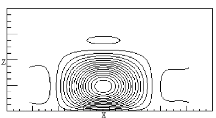
Figure 1: The axial vorticity (the second component of vorticity) contours of the initial value on the symmetry plane. The vertical axis is the $z$-axis, and the horizontal axis is the $x$-axis.

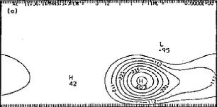
Figure 2: Kerr’s axial vorticity contours of the initial value on the symmetry plane. The vertical axis is the $z$-axis, and the horizontal axis is the $x$-axis. This is Fig. 2(a) of [14].

We should point out that due to the difference between Kerr’s discretization strategies and ours in solving the 3D Euler equations, there is some noticeable difference between the discrete initial condition generated by Kerr’s discretization and the one generated by our pseudo-spectral discretization. In [14], Kerr interpolated the initial condition from the uniform grid to the Chebyshev grid along the $z$-direction and applied extra filtering. This interpolation and extra filtering, which were not provided explicitly in [14], seem to introduce some numerical artifact to Kerr’s discrete initial condition. According to [14] (see the top paragraph of page 1729), “An effect of the initial filter upon the vorticity contours at $t=0$ is a long tail in Fig. 2(a)”. Since our computations are performed on a uniform grid using the pseudo-spectral approximations in all three directions, we do not need to use any interpolation To demonstrate this slight difference between Kerr’s discrete initial condition and ours, we plot the initial vorticity contours along the symmetry plane in Figure 1 using our spectral discretization in all three directions. As we can see, the initial vorticity contours in Figure 1 are essentially symmetric. This is in contrast to the apparent asymmetry in Kerr’s initial vorticity contours as illustrated by Figure 2, which is Fig. 2(a) of [14]. We also present the 3D plot of the vortex tubes at $t=0$ and $t=6$ respectively in Figure 3. We can see that the two initial vortex tubes are essentially symmetric. By time $t=6$, there is already a significant flattening near the center of the tubes.

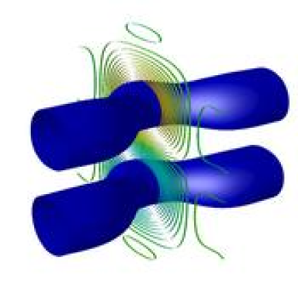
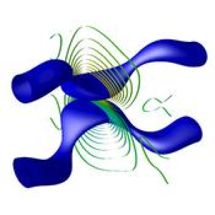
Figure 3: The 3D view of the vortex tube for $t=0$ and $t=6$. The tube is the isosurface at $60\%$ of the maximum vorticity. The ribbons on the symmetry plane are the contours at other different values.

We exploit the symmetry properties of the solution in our computations, and perform our computations on only a quarter of the whole domain. Since the solution appears to be most singular in the $z$ direction, we allocate twice as many grid points along the $z$ direction than along the $x$ direction. The solution is least singular in the $y$ direction. We allocate the smallest resolution in the $y$ direction to reduce the computation cost. In our computations, two typical ratios in the resolution along the $x$, $y$ and $z$ directions are $3:2:6$ and $4:3:8$. Our computations were carried out on the PC cluster LSSC-II in the Institute of Computational Mathematics and Scientific/Engineering Computing of Chinese Academy of Sciences and the Shenteng 6800 cluster in the Super Computing Center of Chinese Academy of Sciences. The maximal memory consumption in our computations is about 120 GBytes.

3 Convergence study of the two numerical methods

We use two numerical methods to compute the 3D Euler equations. The first method is the pseudo-spectral method with the 2/3 dealiasing rule. The second method is the pseudo-spectral method with a high order Fourier smoothing. The only difference between these two methods is in the way we perform the cut-off of the high frequency Fourier modes to control the aliasing error. If $\widehat{v}_{k}$ is the discrete Fourier transform of $v$, then we approximate the derivative of $v$ along the $x_{j}$ direction, $v_{x_{j}}$, by taking the discrete inverse Fourier transform of $ik_{j}\rho(2k_{j}/N_{j})\widehat{v}_{k}$, where $k=(k_{1},k_{2},k_{3})$ and $\rho$ is a high frequency Fourier cut-off function. Here $k_{j}$ is the wave number ($|k_{j}|\leqslant N_{j}/2$) along the $x_{j}$ direction and $N_{j}$ is the total number of grid points along the $x_{j}$ direction. For the pseudo-spectral method with the 2/3 dealiasing rule, the cut-off function $\rho$ is chosen such that $\rho(x)=1$ if $|x|\leq 2/3$, and $\rho(x)=0$ if $2/3<|x|\leq 1$. For the pseudo-spectral method with a high order smoothing, we choose the cut-off function $\rho$ to be a smooth function of the form $\rho(x)\equiv\exp(-\alpha|x|^{m})$ with $\alpha=36$ and $m=36$. The time integration is performed using the classical fourth order Runge-Kutta method. Adaptive time stepping is used to satisfy the CFL stability condition with CFL number equal to $\pi/4$. We use a sequence of resolutions: $768\times 512\times 1536$, $1024\times 768\times 2048$, and $1536\times 1024\times 3072$, to demonstrate the convergence of our numerical computations.

3.1 Comparison of the two methods

It is interesting to make some comparison of the two spectral methods we use. First of all, both methods are of spectral accuracy. The pseudo-spectral method with the 2/3 dealiasing rule has been widely used in the computational fluid dynamics community. It has the advantage of removing the aliasing error completely. On the other hand, when the solution is nearly singular, the Fourier spectrum typically decays very slowly. By cutting off the last 1/3 of the high frequency modes along each direction abruptly, this can introduce oscillations in the physical solution due to the Gibbs phenomenon. In this paper, we will provide solid numerical evidences to demonstrate this effect. On the other hand, the pseudo-spectral method with the high order Fourier smoothing is designed to keep the majority of the Fourier modes unchanged and remove the very high modes to avoid the aliasing error, see Fig. 4 for the profile of $\rho(x)$. We choose $\alpha$ to be $36$ to guarantee that $\rho(2k_{j}/N_{j})$ reaches the level of the round-off error ($O(10^{-16})$) at the highest modes. The order of smoothing, $m$, is chosen to be 36 to optimize the accuracy of the spectral approximation, while still keeping the aliasing error under control. As we can see from Figure 4, the effective modes in our computations are about $12\sim 15\%$ more than those using the standard $2/3$ dealiasing rule. Retaining part of the effective high frequency Fourier modes beyond the traditional 2/3 cut-off position is a special feature of the second method.

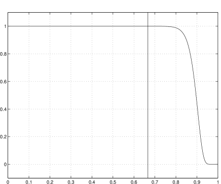
Figure 4: The profile of the Fourier smoothing, $\exp(-36(x)^{36})$, as a function of $x$. The vertical line corresponds to the cut-off mode using the $2/3$ dealiasing rule. We can see that using this Fourier smoothing we keep about $12\sim 15\%$ more modes than those using the 2/3 dealiasing rule.

To compare the performance of the two methods, we perform a careful convergence study for the two methods. In Figure 5, we compare the Fourier spectra of the enstrophy obtained by using the pseudo-spectral method with the $2/3$ dealiasing rule with those obtained by the pseudo-spectral method with the high order smoothing. For a fixed resolution $768\times 512\times 1536$, we can see that the Fourier spectra obtained by the pseudo-spectral method with the high order smoothing retains more effective Fourier modes than those obtained by the spectral method with the $2/3$ dealiasing rule. This can be seen by comparing the results with the corresponding computations using a higher resolution $1024\times 768\times 2048$. Moreover, the pseudo-spectral method with the high order Fourier smoothing does not give the spurious oscillations in the Fourier spectra which are present in the computations using the $2/3$ dealiasing rule near the $2/3$ cut-off point.

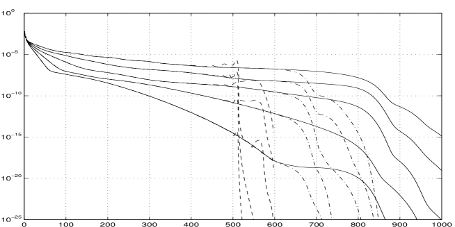
Figure 5: The enstrophy spectra versus wave numbers. We compare the enstrophy spectra obtained using the high order Fourier smoothing method with those using the 2/3 dealiasing rule. The dashed lines and dashed-dotted lines are the enstrophy spectra with the resolution $768\times 512\times 1536$ using the 2/3 dealiasing rule and the Fourier smoothing, respectively. The solid lines are the enstrophy spectra with resolution $1024\times 768\times 2048$ obtained using the high order Fourier smoothing. The times for the spectra lines are at $t=15,16,17,18,19$ respectively.

We perform further comparison of the two methods using the same resolution. In Figure 6, we plot the energy spectra computed by the two methods using resolution $768\times 512\times 1536$. We can see that there is almost no difference in the Fourier spectra generated by the two methods in early times, $t=8,10$, when the solution is still relatively smooth. The difference begins to show near the cut-off point when the Fourier spectra raise above the round-off error level starting from $t=12$. We can see that the spectra computed by the pseudo-spectral method with the 2/3 dealiasing rule introduces noticeable oscillations near the 2/3 cut-off point. The spectra computed by the pseudo-spectral method with the high order smoothing, on the other hand, extend smoothly beyond the 2/3 cut-off point. As we see from Figure 5, a significant portion of those Fourier modes beyond the 2/3 cut-off position are still accurate. In the next subsection, we will demonstrate by a careful resolution study that the pseudo-spectral method with the high order smoothing indeed offers better accuracy than the pseudo-spectral method with the 2/3 dealiasing rule.

Similar comparison can be made in the physical space for the velocity field and the vorticity. In Figure 7, we compare the maximum velocity as a function of time computed by the two methods using resolution $768\times 512\times 1536$. The two solutions are almost indistinguishable. In Figure 8, we plot the maximum vorticity as a function of time. The two solutions agree very well up to $t=18$. The solution obtained by the pseudo-spectral method with the 2/3 dealiasing rule grows slower from $t=18$ to $t=19$. To understand why the two solutions start to deviate from each other toward the end, we examine the contour plot of the axial vorticity in Figures 9 and 10. As we can see, the vorticity computed by the pseudo-spectral method with the 2/3 dealiasing rule already develops small oscillations at $t=17$. The oscillations grow bigger by $t=18$. We note that the oscillations in the axial vorticity contours concentrate near the region where the magnitude of vorticity is close to zero. On the other hand, the solution computed by the spectral method with the high order smoothing is still quite smooth.

Figure 6: The energy spectra versus wave numbers. We compare the energy spectra obtained using the high order Fourier smoothing method with those using the 2/3 dealiasing rule. The dashed lines and solid lines are the energy spectra with the resolution $768\times 512\times 1536$ using the 2/3 dealiasing rule and the Fourier smoothing, respectively. The times for the spectra lines are at $t=8,10,12,14,16,18$ respectively.

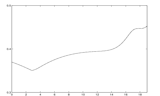
Figure 7: Comparison of maximum velocity as a function of time computed by two methods. The solid line represents the solution obtained by the pseudo-spectral method with the high order smoothing, and the dashed line represents the solution obtained by the pseudo-spectral method with the 2/3 dealiasing rule. The resolution is $768\times 512\times 1536$ for both methods.

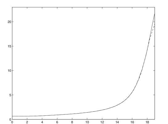
Figure 8: Comparison of maximum vorticity as a function of time computed by two methods. The solid line represents the solution obtained by the pseudo-spectral method with the high order smoothing, and the dashed line represents the solution obtained by the pseudo-spectral method with the 2/3 dealiasing rule. The resolution is $768\times 512\times 1536$ for both methods.

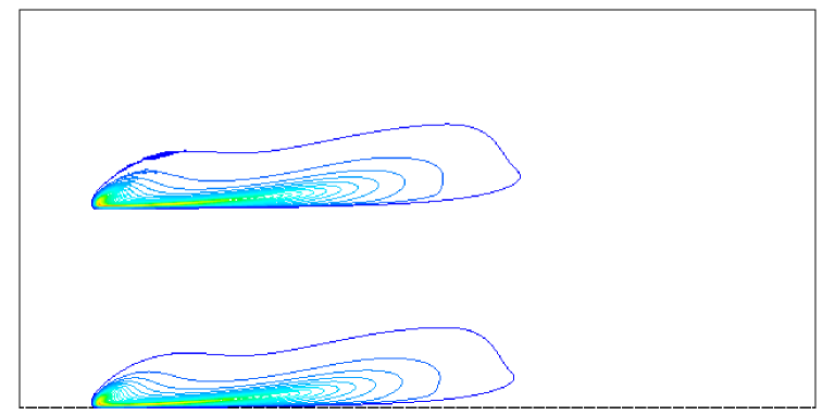
Figure 9: Comparison of axial vorticity contours at $t=17$ computed by two methods. The picture on the top is the solution obtained by the pseudo-spectral method with the 2/3 dealiasing rule, which is shifted by a distance of $\pi$ in $z$ direction, and the picture on the bottom is the solution obtained by the pseudo-spectral method with the high order smoothing. The resolution is $768\times 512\times 1536$ for both methods. The box is the whole $x-z$ computational domain $[-2\pi,2\pi]\times[0,2\pi]$.

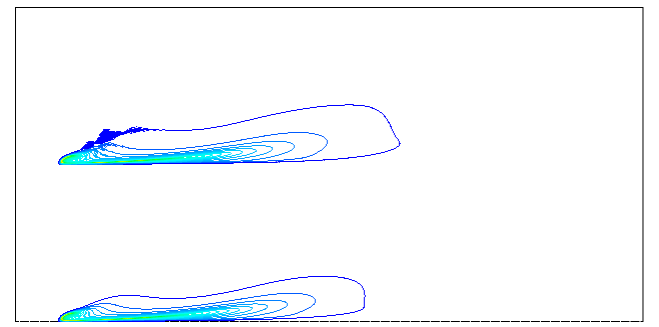
Figure 10: Comparison of axial vorticity contours at $t=18$ computed by two methods. This figure has the same layout as Figure 9. The top picture uses the 2/3 dealiasing rule, while the bottom picture uses the high order smoothing. The resolution is $768\times 512\times 1536$ for both methods.

3.2 Resolution study for the two methods

In this subsection, we perform a resolution study for the two numerical methods using a sequence of resolutions. For the pseudo-spectral method with the high order smoothing, we use the resolutions $768\times 512\times 1536$, $1024\times 768\times 2048$, and $1536\times 1024\times 3072$ respectively. Except for the computation on the largest resolution $1536\times 1024\times 3072$, all computations are carried out from $t=0$ to $t=19$. The computation on the final resolution $1536\times 1024\times 3072$ is started from $t=10$ with the initial condition given by the computation with the resolution $1024\times 768\times 2048$. For the pseudo-spectral method with the 2/3 dealiasing rule, we use the resolutions $512\times 384\times 1024$, $768\times 512\times 1536$ and $1024\times 1024\times 2048$ respectively. The computations using the first two resolutions are carried out from $t=0$ to $t=19$ while the computation on the largest resolution $1024\times 1024\times 2048$ is started at $t=15$ with the initial condition given by the computation with resolution $512\times 512\times 1024$.

First, we perform a convergence study of the enstrophy and energy spectra for the pseudo-spectral method with the high order smoothing at later times (from $t=16$ to $t=19$) using two largest resolutions $1024\times 768\times 2048$, and $1536\times 1024\times 3072$. The results are given in Figures 11 and 12 respectively. They clearly demonstrate the spectral convergence of the spectral method with the high order smoothing.

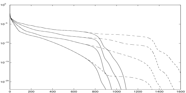
Figure 11: Convergence study for enstrophy spectra obtained by the pseudo-spectral method with high order smoothing using different resolutions. The dashed lines and the solid lines are the enstrophy spectra on resolution $1536\times 1024\times 3072$ and $1024\times 768\times 2048$, respectively. The times for the lines from bottom to top are $t=16,17,18,19$.

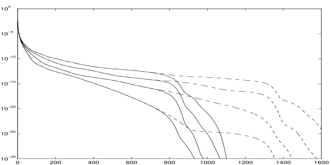
Figure 12: Convergence study for energy spectra obtained by the pseudo-spectral method with high order smoothing using different resolutions. The dashed lines and the solid lines are the energy spectra on resolution $1536\times 1024\times 3072$ and $1024\times 768\times 2048$, respectively. The times for the lines from bottom to top are $t=16,17,18,19$.

To further demonstrate the accuracy of our computations, we compare the maximum vorticity obtained by the pseudo-spectral method with the high order smoothing for three different resolutions: $768\times 512\times 1536$, $1024\times 768\times 2048$, and $1536\times 1024\times 3072$ respectively. The result is plotted in Figure 13. Two conclusions can be made from this resolution study. First, by comparing Figure 13 with Figure 8, we can see that the pseudo-spectral method with the high order smoothing is indeed more accurate than the pseudo-spectral method with the 2/3 dealiasing rule for a given resolution. Secondly, the resolution $768\times 512\times 1536$ is not good enough to resolve the nearly singular solution at later times. However, we observe that the difference of the numerical solution obtained by the resolution $1024\times 768\times 2048$ is very close to that obtained by the resolution $1536\times 1024\times 3072$. This indicates that the vorticity is reasonably well-resolved by our largest resolution $1536\times 1024\times 3072$.

We have also performed a similar resolution study for the maximum velocity in Figure 14. The solutions obtained by the two largest resolutions are almost indistinguishable, which suggests that the velocity is well-resolved by our largest resolution $1536\times 1024\times 3072$.

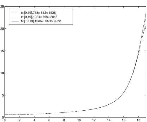
Figure 13: The maximum vorticity $\|\vec{\omega}\|_{\infty}$ in time computed by the pseudo-spectral method with high order smoothing using different resolutions.

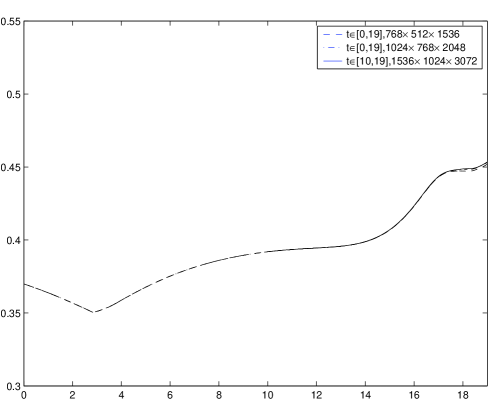
Figure 14: Maximum velocity $\|\vec{u}\|_{\infty}$ in time computed by the pseudo-spectral method with high order smoothing using different resolutions.

Next, we perform a similar resolution study for the pseudo-spectral method with the 2/3 dealiasing rule. The results are very similar to the ones we have obtained for the pseudo-spectral method with the high order smoothing. Here we just present a few representative results. In Figure 15, we plot the enstrophy spectra for a sequence of times from $t=8$ to $t=18$ using different resolutions. The resolutions we use here are $512\times 384\times 1024$, $786\times 512\times 1536$, and $1024\times 1024\times 2048$ respectively. If we compare the Fourier spectra at $t=17$ and $t=18$ (the last two curves in Figure 15), we clearly observe convergence of the enstrophy spectra as we increase our resolutions. On the other hand, the decay of the enstrophy spectra becomes very slow at later times. The oscillations near the 2/3 cut-off point become more and more pronounced as time increases. This abrupt cut-off of high frequency spectra introduces some oscillations in the vorticity contours at later times.

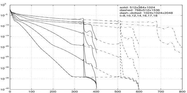
Figure 15: Convergence study for enstrophy spectra obtained by the pseudo-spectral method with the 2/3 dealiasing rule using different resolutions. The solid line is computed with resolution $512\times 384\times 1024$, the dashed line is computed with resolution $786\times 512\times 1536$, and the dashed-dotted line is computed with resolution $1024\times 1024\times 2048$. The times for the lines from bottom to top are $t=8,10,12,14,16,17,18$.

To demonstrate that the two numerical methods converge to the same solution when the solution is nearly singular, we compare the enstrophy spectra computed by the two numerical methods at later times using the largest resolutions that we can afford. For the pseudo-spectral method with the high order smoothing, we use resolution $1536\times 1024\times 3072$. For the pseudo-spectral method with the 2/3 dealiasing rule, we use resolution $1024\times 1024\times 2048$. In Figure 16, we plot the enstrophy spectra for $t=17$, 18, and 18.5 respectively. We observe that the two methods give excellent agreement for those Fourier modes that are not affected by the high frequency cut-off. This shows that the two numerical methods converge to the same solution with spectral accuracy.

Figure 16: The enstrophy spectra versus wave numbers. We compare the enstrophy spectra obtained using the high order Fourier smoothing method with those using the 2/3 dealiasing rule. The dashed lines lines are the enstrophy spectra using the 2/3 dealiasing rule with resolution $1024\times 1024\times 2048$, and the solid lines are the spectra with resolution $1536\times 1024\times 3072$ using the Fourier smoothing. The times for the spectra lines are at $t=17,18,18.5$ respectively.

We have performed a similar convergence study for the pseudo-spectral method with the 2/3 dealiasing in the physical space for the maximum vorticity. The result is given in Figure 17. As we can see, the computation with a higher resolution gives faster growth in the maximum vorticity. This is also what we observed earlier for the pseudo-spectral method with the high order smoothing. As we will see in the next section, the maximum vorticity grows almost like doubly exponential in time. To capture this rapid dynamic growth of maximum vorticity, we must have sufficient resolution to resolve the nearly singular solution of the Euler equations at later times.

The resolution study given by Figure 17 suggests that the maximum vorticity is reasonably resolved by resolution $768\times 512\times 1536$ before $t=18$. It is interesting to note that at $t=17$, small oscillations have already appeared in the vorticity contours in the region where the magnitude of vorticity is small, see Figure 9. Apparently, the small oscillations in the region where the vorticity is close to zero in magnitude have not yet polluted the accuracy of the maximum vorticity in a significant way. Note that there is no oscillation developed in the vorticity contours obtained by the pseudo-spectral method with the high order smoothing at this time. From Figure 8, we know that the maximum vorticity computed by the two methods agrees reasonably well with each other before $t=18$. This shows that the two methods can still approximate the maximum vorticity reasonably well with resolution $768\times 512\times 1536$ before $t=18$.

The resolution study given by Figure 17 also suggests that the the computation obtained by the pseudo-spectral method with the 2/3 dealiasing rule using resolution $768\times 512\times 1536$ is significantly under-resolved after $t=18$. This is also supported by the appearance of the relatively large oscillations in the vorticity contours at $t=18$ from Figure 10. It is interesting to note from Figure 8 that the computational results obtained by the two methods with resolution $768\times 512\times 1536$ begin to deviate from each other precisely around $t=18$. By comparing the result from Figure 8 with that from Figure 17, we confirm again that for a given resolution, the pseudo-spectral method with the high order smoothing gives a more accurate approximation than the pseudo-spectral method with the 2/3 dealiasing rule.

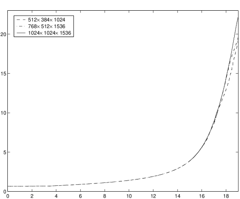
Figure 17: The maximum vorticity $\|\vec{\omega}\|_{\infty}$ in time computed by the pseudo-spectral method with the 2/3 dealiasing rule using different resolutions.

4 Analysis of computational results

In this section, we will present a series of numerical results to reveal the nature of the nearly singular solution of the 3D Euler equations, and compare our results with those obtained by Kerr in [14, 17]. Based on the convergence study we have performed in the previous section, we will present only those numerical results which are computed by the pseudo-spectral method with the high order smoothing using the largest resolution $1536\times 1024\times 3072$.

4.1 Review of Kerr’s results

In [14], Kerr presented numerical evidence which suggested a finite time singularity of the 3D Euler equations for two perturbed antiparallel vortex tubes. He used a pseudo-spectral discretization in the $x$ and $y$ directions, and a Chebyshev method in the $z$ direction with resolution of order $512\times 256\times 192$. His computations showed that the growth of the peak vorticity, the peak axial strain, and the enstrophy production obey $(T-t)^{-1}$ with $T=18.9$. Kerr stated in his paper [14] (see page 1727) that his numerical results shown after $t=17$ and up to $t=18$ were “not part of the primary evidence for a singularity” due to the lack of sufficient numerical resolution and the presence of noise in the numerical solutions. In his recent paper [17] (see also [15, 16]), Kerr applied a high wave number filter to the data obtained in his original computations to “remove the noise that masked the structures in earlier graphics” presented in [14]. With this filtered solution, he presented some scaling analysis of the numerical solutions up to $t=17.5$. The velocity field was shown to blow up like $O((T-t)^{-1/2})$ with $T$ being revised to $T=18.7$.

4.2 Maximum vorticity growth

From the resolution study we present in Figure 13, we find that the maximum vorticity increases rapidly from the initial value of $0.669$ to $23.46$ at the final time $t=19$, a factor of 35 increase from its initial value. Kerr’s computations predicted a finite time singularity at $T=18.7$. Our computations show no sign of finite time blowup of the 3D Euler equations up to $T=19$, beyond the singularity time predicted by Kerr. We use three different resolutions, i.e. $768\times 512\times 1536$, $1024\times 768\times 2048$, and $1536\times 1024\times 3072$ respectively in our computations. As we can see, the agreement between the two successive resolutions is very good with only mild disagreement toward the end of the computations. This indicates that a very high space resolution is indeed needed to capture the rapid growth of maximum vorticity at the later stage of the computations.

In order to understand the nature of the dynamic growth in vorticity, we examine the degree of nonlinearity in the vortex stretching term. In Figure 18, we plot the quantity, $\|\xi\cdot\nabla\vec{u}\cdot\vec{\omega}\|_{\infty}$, as a function of time, where $\xi$ is the unit vorticity vector. If the maximum vorticity indeed blew up like $O((T-t)^{-1})$, as alleged in [14], this quantity should have been quadratic as a function of maximum vorticity. We find that there is tremendous cancellation in this vortex stretching term. It actually grows slower than $C\|\vec{\omega}\|_{\infty}\log(\|\vec{\omega}\|_{\infty})$, see Figure 18. It is easy to show that such weak nonlinearity in vortex stretching would imply only doubly exponential growth in the maximum vorticity. Indeed, as demonstrated by Figure 19, the maximum vorticity does not grow faster than doubly exponential in time. In fact, the growth slows down toward the end of the computation, which indicates that there is stronger cancellation taking place in the vortex stretching term.

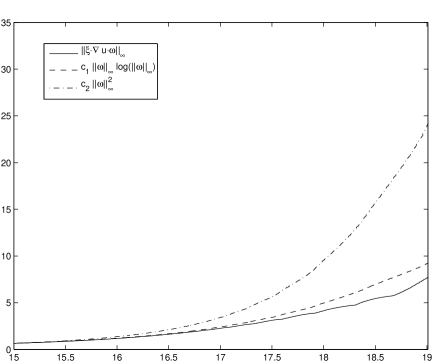
Figure 18: Study of the vortex stretching term in time, resolution $1536\times 1024\times 3072$. We take $c_{1}=1/8.128$, $c_{2}=1/23.24$ to match the same starting value for all three plots.

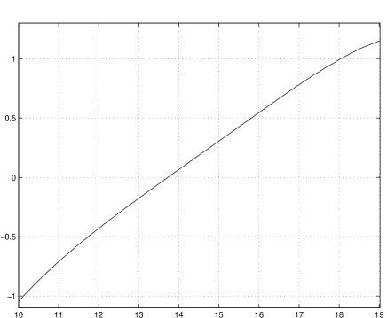
Figure 19: The plot of $\log\log\|\omega\|_{\infty}$ vs time, resolution $1536\times 1024\times 3072$.

We remark that for vorticity that grows as rapidly as doubly exponential in time, one may be tempted to fit the maximum vorticity growth by $c/(T-t)$ for some $T$. Indeed, if we choose $T=18.7$ as suggested by Kerr in [17], we find a reasonably good fit for the maximum vorticity as a function of $c/(T-t)$ for the period $15\leq t\leq 17$. We plot the scaling constant $c$ in Figure 20. As we can see, $c$ is close to a constant for $15\leq t\leq 17$. To conclude that the 3D Euler equations indeed develop a finite time singularity, one must demonstrate that such scaling persists as $t$ approaches to $T$. As we can see from Figure 20, the scaling constant $c$ decreases rapidly to zero as $t$ approaches to the alleged singularity time $T$. Therefore, the fitting of $\|\vec{\omega}\|_{\infty}\approx O((T-t)^{-1})$ is not correct asymptotically.

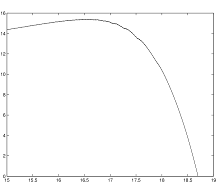
Figure 20: Scaling constant in time for the fitting $\|\omega\|_{\infty}\approx c/(T-t)$, $T=18.7$.

4.3 Velocity profile

One of the important findings of our computations is that the velocity field is actually bounded by 1/2 up to $T=19$. This is in contrast to Kerr’s computations in which the maximum velocity was shown to blow up like $O((T-t)^{-1/2})$ [15, 17]. We plot the maximum velocity as a function of time using different resolutions in Figure 14. The computation obtained by resolution $1024\times 768\times 2048$ and the one obtained by resolution $1536\times 1024\times 3072$ are almost indistinguishable. The fact that the velocity field is bounded is significant. With the velocity field being bounded, the non-blowup theory of Deng-Hou-Yu [8] can be applied, which implies non-blowup of the 3D Euler equations up to $T$. We refer to [13] for more discussions.

4.4 Local vorticity structure

In this subsection, we would like to examine the local vorticity structure near the region of the maximum vorticity. To illustrate the development in the symmetry plane, we show a series of vorticity contours near the region of the maximum vorticity at late times in a manner similar to the results presented in [14]. For some reason, Kerr scaled his axial vorticity contours by a factor of 5 along the $z$-direction. Noticeable oscillations already develop in Kerr’s axial vorticity contours at $t=15$ and $t=17$, see Figure 22. To compare with Kerr’s results, we scale the vorticity contours in the $x-z$ plane by a factor of 5 in the $z$-direction. The results at $t=15$ and $t=17$ are plotted in Figure 21. The results are in qualitative agreement with Kerr’s results, except that our computations are better resolved and do not suffer from the noise and oscillations which are present in Kerr’s vorticity contours.

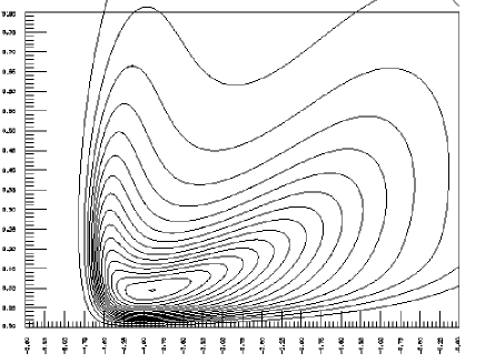
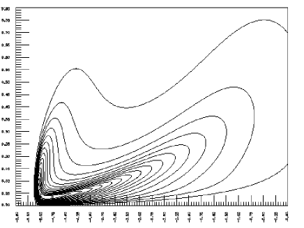
Figure 21: The contour of axial vorticity around the maximum vorticity on the symmetry plane at $t=15$ (on the left) and $t=17$ (on the right). The vertical axis is the $z$-axis, and the horizontal axis is the $x$-axis. The figure is scaled in $z$ direction by a factor of $5$ to compare with Figure 4 in [14].

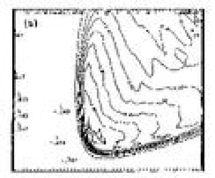
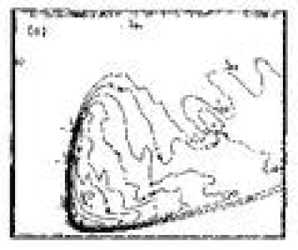
Figure 22: Kerr’s axial vorticity contours on the symmetry plane at $t=15$ (on the left) and $t=17$ (on the right). These are from Figure 4 in [14].

In order to see better the dynamic development of the local vortex structure, we plot a sequence of vorticity contours on the symmetry plane at $t=17.5,18,18.5,$ and $19$ respectively in Figure 23. The pictures are plotted using the original length scales, without the scaling by a factor of 5 in the $z$ direction as in Figure 21. From these results, we can see that the vortex sheet is compressed in the $z$ direction. It is clear that a thin layer (or a vortex sheet) is formed dynamically. The head of the vortex sheet begins to roll up around $t=16$. Here the head of the vortex sheet refers to the region extending above the vorticity peak just behind the leading edge of the vortex sheet [14]. By the time $t=19$, the head of the vortex sheet has traveled backward for quite a distance and away from the dividing plane. The vortex sheet has been compressed quite strongly along the $z$-direction. In order to resolve this nearly singular layer structure, we use 3072 grid points along the $z$-direction, which gives about 16 grid points across the layer at $t=18$ and about 8 grid points across the layer at $t=19$. In comparison, the 192 Chebyshev grid points along the $z$-direction in Kerr’s computations would not be sufficient to resolve the rolled-up portion of the vortex sheet.

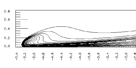
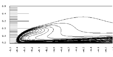
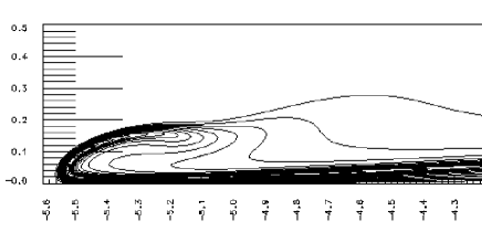
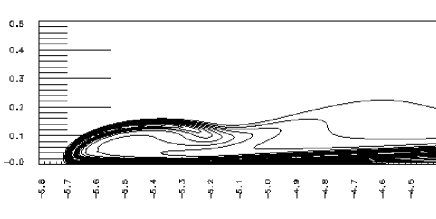
Figure 23: The contour of axial vorticity around the maximum vorticity on the symmetry plane (the $x-z$ plane) at $t=17.5,18,18.5,19$.

We also plot the isosurface of vorticity near the region of the maximum vorticity in Figures 24 and 25 to illustrate the dynamic roll-up of the vortex sheet near the region of the maximum vorticity. The isosurface of vorticity in Figure 24 is set at $0.6\times\|\vec{\omega}\|_{\infty}$. Figure 24 gives the local vorticity structure at $t=17$. If we scale the local roll-up region on the left hand side next to the box by a factor of 4 along the $z$ direction, as was done in [17], we would obtain a local roll-up structure which is qualitatively similar to Figure 1 in [17]. In Figure 25, we show the local vorticity structure for $t=18$ and $t=19$. In both figures, the isosurface is set at $0.5\times\|\vec{\omega}\|_{\infty}$. We can see that the vortex sheets have rolled up and traveled backward in time away from the dividing plane. Moreover, we observe that the vortex lines near the region of maximum vorticity are relatively straight and the unit vorticity vectors seem to be quite regular. On the other hand, the inner region containing the maximum vorticity does not seem to shrink to zero at a rate of $(T-t)^{1/2}$, as predicted in [17]. The length and the width of the vortex sheet are still $O(1)$, although the thickness of the vortex sheet becomes quite small.

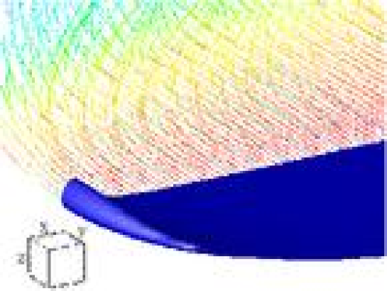
Figure 24: The local 3D vortex structure and vortex lines around the maximum vorticity at $t=17$. The size of the box on the left is $0.075^{3}$ to demonstrate the scale of the picture. The isosurface is set at $0.6\times\|\vec{\omega}\|_{\infty}$.

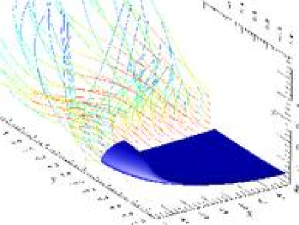
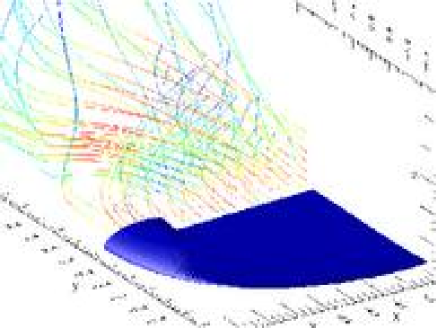
Figure 25: The local 3D vortex structures and vortex lines around the maximum vorticity at $t=18$ (on the left) and $t=19$ (on the right). The isosurface is set at $0.5\times\|\vec{\omega}\|_{\infty}$.

Another interesting question is how the vorticity vector aligns with the eigenvectors of the deformation tensor, which is defined as $M\equiv\displaystyle\frac{1}{2}(\nabla\vec{u}+\nabla^{T}\vec{u})$. In Table 1, we document the alignment information of the vorticity vector around the point of maximum vorticity with resolution $1536\times 1024\times 3072$. In this table, $\lambda_{i}$ ($i=1,2,3$) is the $i$-th eigenvalue of $M$, $\theta_{i}$ is the angle between the $i$-th eigenvector of $M$ and the vorticity vector. One can see clearly that for $16\leq t\leq 19$ the vorticity vector at the point of maximum vorticity is almost perfectly aligned with the second eigenvector of $M$. The angle between the vorticity vector and the second eigenvector is very small throughout this time interval. Note that the second eigenvalue, $\lambda_{2}$, is positive and is about 20 times smaller in magnitude than the largest and the smallest eigenvalues. This dynamic alignment of the vorticity vector with the second eigenvector of the deformation tensor is another indication that there is a dynamic depletion of vortex stretching.

time	$|\omega|$	$\lambda_{1}$	$\theta_{1}$	$\lambda_{2}$	$\theta_{2}$	$\lambda_{3}$	$\theta_{3}$
16.012295	5.628002	-1.508771	89.992936	0.206199	0.007159	1.302352	89.998852
16.515890	7.016002	-1.864394	89.995940	0.232299	0.010438	1.631355	89.990387
17.013589	8.910001	-2.322629	89.998141	0.254699	0.006815	2.066909	89.993445
17.515769	11.430017	-2.630440	89.969954	0.224305	0.085053	2.415185	89.920433
18.011609	14.890004	-3.625738	89.969613	0.257302	0.036607	3.378515	89.979590
18.516346	19.130010	-4.501348	89.966725	0.246305	0.036617	4.274913	89.984720
19.014394	23.590012	-5.477438	89.966055	0.247906	0.034472	5.258292	89.994005

Table 1: The alignment of the vorticity vector and the eigenvectors of $M$ around the point of maximum vorticity with resolution $1536\times 1024\times 3072$. Here, $\lambda_{i}$ ($i=1,2,3$) is the $i$-th eigenvalue of $M$, $\theta_{i}$ is the angle between the $i$-th eigenvector of $M$ and the vorticity vector. One can see that the vorticity vector is aligned very well with the second eigenvector of $M$

.

5 Concluding Remarks

We investigate the interaction of two perturbed vortex tubes for the 3D Euler equations using Kerr’s initial condition [14]. We use both the pseudo-spectral method with the standard 2/3 dealiasing rule and the pseudo-spectral method with a 36th order Fourier smoothing. We perform a careful resolution study to demonstrate the convergence of both methods. Our numerical computations demonstrate that while both methods converge to the same solution under resolution study, the pseudo-spectral method with the 36th order Fourier smoothing offers better computational accuracy for a given resolution. Moreover, we find that the pseudo-spectral method with the 36th order Fourier smoothing is more effective in reducing the numerical oscillations due to the Gibbs phenomenon while still keeping the aliasing error under control.

Our numerical study indicates that there is a very subtle dynamic depletion of vortex stretching. The maximum vorticity is shown to grow no faster than doubly exponential in time up to $T=19$, beyond the singularity time predicted by Kerr in [14]. The velocity field is shown to be bounded throughout the computations. Vortex lines near the region of the maximum vorticity are quite regular. We provide numerical evidence that the vortex stretching term is only weakly nonlinear and is bounded by $\|\vec{\omega}\|_{\infty}\log(\|\vec{\omega}\|_{\infty})$. This implies that there is tremendous dynamic cancellation in the nonlinear vortex stretching term. With the velocity field being bounded and the vortex lines being regular near the region of the maximum vorticity, the non-blowup conditions of Deng-Hou-Yu [8] are satisfied. This provides a theoretical support for our computational results and sheds some light to our understanding of the dynamic depletion of vortex stretching.

Finally, we would like to mention that we have carried out a rigorous convergence study of the two numerical methods we consider in this paper for the one-dimensional Burgers equation. The Burgers equation shares some essential numerical difficulties with the the 3D Euler equations that we consider here. It has the same type of quadratic nonlinearity in the convection term and it is known that it can form a shock singularity in a finite time. An important advantage of the Burgers equation is that we have an analytic solution formula which can be solved numerically up to the machine precision by using the Newton iterative method. Using this semi-analytical solution, we have computed the solution very close to the shock singularity time and documented the errors of both numerical methods using very large resolutions. The computational results we obtain on the Burgers equation completely support the convergence study of the two numerical methods for the 3D Euler equations that we present in this paper. The performance of these two numerical methods and their convergence property for the 1D Burgers equation are basically the same as those for the 3D Euler equations. The detail of this result will be reported elsewhere.

Acknowledgments. We would like to thank Prof. Lin-Bo Zhang from the Institute of Computational Mathematics in Chinese Academy of Sciences for providing us with the computing resource to perform this large scale computational project. Additional computing resource was provided by the Center of Super Computing Center of Chinese Academy of Sciences. We also thank Prof. Robert Kerr for providing us with his Fortran subroutine that generates his initial data. This work was in part supported by NSF under the NSF FRG grant DMS-0353838 and ITR Grant ACI-0204932. Part of this work was done while Hou visited the Academy of Systems and Mathematical Sciences of CAS in the summer of 2005 as a member of the Oversea Outstanding Research Team for Complex Systems.

References

- [1] C. Anderson and C. Greengard, The vortex ring merger problem at infinite reynolds number, Comm. Pure Appl. Maths 42 (1989), 1123.
- [2] O. N. Boratav and R. B. Pelz, Direct numerical simulation of transition to turbulence from a high-symmetry initial condition, Phys. Fluids 6 (1994), no. 8, 2757–2784.
- [3] O. N. Boratav, R. B. Pelz, and N. J. Zabusky, Reconnection in orthogonally interacting vortex tubes: Direct numerical simulations and quantifications, Phys. Fluids A 4 (1992), no. 3, 581–605.
- [4] R. Caflisch, Singularity formation for complex solutions of the 3D incompressible Euler equations, Physica D 67 (1993), 1–18.
- [5] A. Chorin, The evolution of a turbulent vortex, Commun. Math. Phys. 83 (1982), 517.
- [6] P. Constantin, Geometric statistics in turbulence, SIAM Review 36 (1994), 73.
- [7] P. Constantin, C. Fefferman, and A. Majda, Geometric constraints on potentially singular solutions for the 3-D Euler equation, Commun. in PDEs. 21 (1996), 559–571.
- [8] J. Deng, T. Y. Hou, and X. Yu, Geometric properties and non-blowup of 3-D incompressible Euler flow, Comm. in PDEs. 30 (2005), no. 1, 225–243.
- [9] , Improved geometric conditions for non-blowup of 3D incompressible Euler equation, Comm. in PDEs. 31 (2006), no. 2, 293–306.
- [10] V. M. Fernandez, N. J. Zabusky, and V. M. Gryanik, Vortex intensification and collapse of the Lissajous-Elliptic ring: Single and multi-filament Biot-Savart simulations and visiometrics, J. Fluid Mech. 299 (1995), 289–331.
- [11] R. Grauer, C. Marliani, and K. Germaschewski, Adaptive mesh refinement for singular solutions of the incompressible Euler equations, Phys. Rev. Lett. 80 (1998), 19.
- [12] R. Grauer and T. Sideris, Numerical computation of three dimensional incompressible ideal fluids with swirl, Phys. Rev. Lett. 67 (1991), 3511.
- [13] T. Y. Hou and R. Li, Dynamic depletion of vortex stretching and non-blowup of the 3-D incompressible Euler equations, accepted by J. Nonlinear Science. (2006).
- [14] R. M. Kerr, Evidence for a singularity of the three dimensional, incompressible Euler equations, Phys. Fluids 5 (1993), no. 7, 1725–1746.
- [15] , Euler singularities and turbulence, 19th ICTAM Kyoto ’96 (T. Tatsumi, E. Watanabe, and T. Kambe, eds.), Elsevier Science, 1997, pp. 57–70.
- [16] , The outer regions in singular Euler, Fundamental problematic issues in turbulence (Birkhäuser) (Tsnober and Gyr, eds.), 1999.
- [17] , Velocity and scaling of collapsing Euler vortices, Phys. Fluids 17 (2005), 075103–114.
- [18] R. M. Kerr and F. Hussain, Simulation of vortex reconnection, Physica D 37 (1989), 474.
- [19] M. V. Melander and F. Hussain, Cross linking of two antiparallel vortex tubes, Phys. Fluids A (1989), 633–636.
- [20] R. B. Pelz, Locally self-similar, finite-time collapse in a high-symmetry vortex filament model, Phys. Rev. E 55 (1997), no. 2, 1617–1626.
- [21] A. Pumir and E. E. Siggia, Collapsing solutions to the 3-D Euler equations, Phys. Fluids A 2 (1990), 220–241.
- [22] M. J. Shelley, D. I. Meiron, and S. A. Orszag, Dynamical aspects of vortex reconnection of perturbed anti-parallel vortex tubes, J. Fluid Mech. 246 (1993), 613–652.