Channeling chaotic transport in a wave-particle experiment

Abstract

[A numerical and experimental study of a control method aimed at channeling chaos by building barriers in phase space is performed on a paradigm for wave-particle interaction, i.e., a traveling wave tube. Control of chaotic diffusion is achieved by adding small apt modifications to the system with a low additional cost of energy. This modification is realized experimentally through additional waves with small amplitudes. Robustness of the method is investigated both numerically and experimentally.]

I Introduction

The interaction of a beam of charged particles with electromagnetic waves is ubiquitous in physics, and it is central to many useful devices such as particle accelerators, plasma fusion experiments or free electron lasers. In these experimental set-ups, the waves are used to accelerate the particles or to guide them by assigning a specific mean trajectory. However, the dynamics of these systems is usually characterized by the competition of many degrees of freedom and thus, shows generically chaotic behaviors. Such behaviors represent a limit to the achievement of high performances in these devices. Consequently, there has been a growing interest in controlling chaos which here means to reduce it when and where it is undesirable and to increase it when it is useful.

The sensitivity of chaotic systems to small perturbations triggered a strong interdisciplinary effort to control chaos c1 ; c2 ; c3 ; c4 ; c5 ; c6 ; c7 ; c8 . After the seminal work on optimal control by Pontryagin c9 , efficient methods were proposed for controlling chaotic systems by nudging targeted trajectories c10 ; c11 ; c12 ; c13 ; c14 . However, for many body experiments such methods are hopeless due to the high number of trajectories to deal with simultaneously.

It was recently proposed a local control method chan06 which aims at building barriers in phase space and hence confines all the trajectories rather than following them individually. These barriers are stable structures in phase space like for instance invariant tori, which are generically broken by the perturbation. The reduction of chaotic behaviors is achieved by using a small apt perturbation of the system which keeps its Hamiltonian structure.

In this article, we consider a traveling wave tube (TWT) specially designed to study wave particle interaction which is used to investigate experimentally the control method and its robustness. The dynamics in this experimental apparatus can be accurately represented using a Hamiltonian which describes the motion of a charged particle (with unit mass) interacting with two electrostatic waves c16  :

$$H(p,x,t) = \frac{p^{2}}{2}+\varepsilon_{1}\cos(k_{1}x-\omega_{1}t+\varphi_{1})$$ (1)

$$+\varepsilon_{2}\cos(k_{2}x-\omega_{2}t+\varphi_{2}),$$

where $(p,x)\in{\mathbb{R}}\times[0,L]$ are the momentum and position of the particle in a tube of length $L$. The amplitudes, wave numbers, frequencies and phases of the two waves are denoted respectively $\varepsilon_{i}$, $k_{i}$, $\omega_{i}$ and $\varphi_{i}$ for $i=1,2$. We notice that the beam intensity is sufficiently low such that the wave growth rate is negligible upon the length of the experiment that is we are in the test-particle regime.

Generically, the dynamics of the particles governed by Hamiltonian (1) is a mixture of regular and chaotic behaviors, mainly depending on the amplitudes of the waves. The Chirikov parameter Chirikov defined as the ratio between the two half-width of the primary resonances by the distance between these resonances, i.e.,

$$s=\frac{{2}(\sqrt{{|\varepsilon_{1}}|}+\sqrt{{|\varepsilon_{2}|}})}{|{\omega_{2}}/{k_{2}}-{\omega_{1}}/{k_{1}}|},$$ (2)

gives a first rough approximation of the chaoticity degree of the system. Hamiltonian (1) has a typical behavior of integrable system for small values of this parameter ($s$$\ll 1$). For large enough amplitudes of the waves ($s\sim 1$), large scale chaos occurs in phase space. As a consequence, the particle can have an arbitrary velocity in between the two phase velocities of the waves ($\omega_{2}/k_{2}$ and $\omega_{1}/k_{1}$). In this TWT, such typical chaotic behavior has been observed directly Macor1 . This chaotic diffusion of the particles in phase space can be reduced by using an apt control term which consists here as an additional wave (or more generally a set of waves) of small amplitude. The characteristics of this additional wave are computed explicitly, and then the wave is injected in addition to the two others. The results presented in this article were announced in Ref. c18 .

The paper is organized as follows : The control method is briefly recalled in Sec. II.1 and its application to the considered Hamiltonian is presented in Sec. II.2. Numerical investigations of the effect of the control term and its robustness are reported in Secs. II.3 and II.4. In Sec. III.1, a description of the experimental set-up precedes the results of the implementation of the control term shown in Sec. III.2 as well as its robustness in Sec. III.3.

II Local control method applied to a two wave model

The Hamiltonian of an integrable system can be locally written as a function $H_{0}({\bf A})$ of the action variables ${\bf A}=(A_{1},A_{2},\ldots,A_{d})\in{\mathbb{R}}^{d}$, i.e. it does not depend on the conjugate angle variables ${\bm{\theta}}=(\theta_{1},\theta_{2},\ldots,\theta_{d})\in{\mathbb{T}}^{d}={\mathbb{R}}^{d}/(2\pi{\mathbb{Z}})^{d}$, where ${\mathbb{T}}^{d}$ is the $d$-dimensional torus parameterized by $[0,2\pi[^{d}$. The equations of motion for $H_{0}({\bf A})$ show that the action variables are constant, and consequently the trajectories with given actions $\bf{A}$ are confined to evolve on a $d$-dimensional torus with frequency vector ${\bm{\omega}}_{0}({\bf A})=\partial H_{0}/\partial{\bf A}$. The dynamics on this torus is periodic or quasi-periodic: ${\bm{\theta}}(t)={\bm{\omega}}_{0}({\bf A})t+{\bm{\theta}}(0)$ with frequency vector ${\bm{\omega}}_{0}({\bf A})$. In the particular case given by Hamiltonian (1) an integrable situation is given by $\varepsilon_{1}=\varepsilon_{2}=0$ so that the dynamics of the integrable system $H=p^{2}/2$ is characterized by constant velocity ($p=const$). A monokinetic beam of charged particles remains monokinetic.

If the system described by $H_{0}$ is perturbed, i.e. we consider the Hamiltonian

$$H({\bf A},{\bm{\theta}})=H_{0}({\bf A})+V({\bf A},{\bm{\theta}}),$$

the integrability is generically lost and the system becomes chaotic. Even if KAM theorem establishes the stability with respect to small perturbations of invariant tori with a sufficiently incommensurate frequency vector these tori are destroyed when the amplitude of the perturbation $V$ is large enough. The break-up of invariant tori leads to a loss of stability of the system until the last invariant torus of the integrable case is destroyed and then large scale diffusion occurs in phase space. In the case of a beam of charged particles whose dynamics is given by Hamiltonian (1), for $\varepsilon_{1}$, $\varepsilon_{2}$ sufficiently large, an initially monokinetic beam will spread in velocity due to this diffusion.

II.1 Expression of the local control term

The aim is to provide an explicit expression for an additional perturbation such that a specific invariant torus is reconstructed in the modified system. We state here the main result which has been extensively described in Ref. chan06  : We consider Hamiltonian systems written as

$$H({\bf A},{\bm{\theta}})={\bm{\omega}}\cdot{\bf A}+W({\bf A},{\bm{\theta}}),$$

where $\bm{\omega}$ is a non-resonant vector of ${\mathbb{R}}^{d}$. Without loss of generality, we consider a region near ${\bf A}={\bf 0}$ (by translation of the actions) and, since the Hamiltonian is nearly integrable, the perturbation $W$ has constant and linear parts in actions of order $\varepsilon$, i.e.

$$W({\bf A},{\bm{\theta}})=\varepsilon v({\bm{\theta}})+\varepsilon{\bf w}({\bm{\theta}})\cdot{\bf A}+Q({\bf A},{\bm{\theta}}),$$ (3)

where $Q$ is of order $O(\|{\bf A}\|^{2})$. We notice that for $\varepsilon=0$, the Hamiltonian $H$ has an invariant torus with frequency vector ${\bm{\omega}}$ at ${\bf A}={\bf 0}$ for any $Q$ not necessarily small. The controlled Hamiltonian we construct is

$$H_{c}({\bf A},{\bm{\theta}})={\bm{\omega}}\cdot{\bf A}+W({\bf A},{\bm{\theta}})+f({\bm{\theta}}).$$ (4)

The control term $f$ we construct only depends on the angle variables and is given by

$$f({\bm{\theta}})=W({\bf 0},{\bm{\theta}})-W\left(-\Gamma\partial_{\bm{\theta}}W({\bf 0},{\bm{\theta}}),{\bm{\theta}}\right),$$ (5)

where $\partial_{\bm{\theta}}$ is the derivative operator with respect to $\bm{\theta}$, and $\Gamma$ is a linear operator defined as a pseudo-inverse of ${\bm{\omega}}\cdot\partial_{\bm{\theta}}$, i.e. acting on $W=\sum_{{\bf k}}W_{{\bf k}}{\mathrm{e}}^{i{\bf k}\cdot{\bm{\theta}}}$ as

$$\Gamma W=\sum_{{\bm{\omega}}\cdot{\bf k}\not=0}\frac{W_{{\bf k}}}{i{\bm{\omega}}\cdot{\bf k}}{\mathrm{e}}^{i{\bf k}\cdot{\bm{\theta}}}.$$

Note that $f$ is of order $\varepsilon^{2}$. For any function $W$, Hamiltonian (4) has an invariant torus with frequency vector close to ${\bm{\omega}}$. The equation of the torus which is restored by the addition of $f$ is

$${\bf A}=-\Gamma\partial_{\bm{\theta}}W({\bf 0},{\bm{\theta}}),$$ (6)

which is of order $\varepsilon$ for $W$ given by Eq. (3)

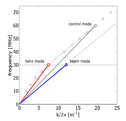
Figure 1: TWT dispersion relation (circles) with the helix mode at 30 MHz (square) and the beam mode at the same frequency but with propagation velocity choose equal to about $2.5\times 10^{6}$ m/s (triangle); the control wave corresponds to the beating of these two modes

II.2 Computation of the control term for a two wave system

We consider Hamiltonian (1) with two waves, where the wavenumbers are chosen according to a dispersion relation $k_{1}=K(\omega_{1})$ and $k_{2}=K(\omega_{2})$ plotted on Fig. 1.

In order to compute $f$, Hamiltonian (1) with 1.5 degrees of freedom is mapped into an autonomous Hamiltonian with two degrees of freedom by considering that $t\mbox{ mod }2\pi$ is an additional angle variable. We denote $E$ its conjugate action. The autonomous Hamiltonian is

$$H(E,p,x,t) = E+\frac{p^{2}}{2}+\varepsilon_{1}\cos(k_{1}x-\omega_{1}t+\varphi_{1})$$ (7)

$$+\varepsilon_{2}\cos(k_{2}x-\omega_{2}t+\varphi_{2}).$$

Then, the momentum $p$ is shifted by $\omega$ in order to define a local control in the region $p\approx 0$. The Hamiltonian is rewritten as

$$H = E+\omega p+\varepsilon_{1}\cos(k_{1}x-\omega_{1}t+\varphi_{1})$$ (8)

$$+\varepsilon_{2}\cos(k_{2}x-\omega_{2}t+\varphi_{2})+\frac{p^{2}}{2}.$$

We rewrite Hamiltonian (8) into the form (3)  where:

$$\varepsilon v(x,t)=\varepsilon_{1}\cos(k_{1}x-\omega_{1}t+\varphi_{1})+\varepsilon_{2}\cos(k_{2}x-\omega_{2}t+\varphi_{2}),$$

$$w(x,t)=0,$$

$$Q(p,x,t)=p^{2}/2.$$

The frequency vector of the selected invariant torus is ${\bm{\omega}}=(\omega,1)$. From Eq. (5) we have that $f$ is given by

$$f(x,t)=-\frac{\varepsilon^{2}}{2}(\Gamma\partial_{x}v)^{2},$$

which is

$$f(x,t)= -\frac{1}{2}\big{[}\frac{\varepsilon_{1}k_{1}}{\omega k_{1}-\omega_{1}}\cos(k_{1}x-\omega_{1}t+\varphi_{1})$$ (9)

$$+\frac{\varepsilon_{2}k_{2}}{\omega k_{2}-\omega_{2}}\cos(k_{2}x-\omega_{2}t+\varphi_{2})\big{]}^{2},$$

provided $\omega\neq\omega_{1}/k_{1}$ and $\omega\neq\omega_{2}/k_{2}$. Adding this exact control term to Hamiltonian (1), the following invariant rotational torus is restored :

$$p(x,t) = \omega-\frac{\varepsilon_{1}k_{1}}{\omega k_{1}-\omega_{1}}\cos(k_{1}x-\omega_{1}t+\varphi_{1})$$ (10)

$$-\frac{\varepsilon_{2}k_{2}}{\omega k_{2}-\omega_{2}}\cos(k_{2}x-\omega_{2}t+\varphi_{2}).$$

This barrier of diffusion prevents a beam of particles to diffuse everywhere in phase space. We emphasize that the barrier persists for all the magnitudes of the waves $(\varepsilon_{1},\varepsilon_{2})$.

The control term (9) has four Fourier modes, $(2k_{1},-2\omega_{1})$, $(2k_{2},-2\omega_{2})$, $((k_{1}+k_{2}),-(\omega_{1}+\omega_{2}))$ and $((k_{1}-k_{2}),-(\omega_{1}-\omega_{2}))$. If we want to restore an invariant torus in between the two primary resonances approximately located at $p\approx\omega_{1}/k_{1}$ and $p\approx\omega_{2}/k_{2}$, the frequency $\omega$ has to be chosen between the two group velocities of the waves. If we consider a beam of particles with a velocity in between the velocities of the waves, i.e., $v_{1}=\omega_{1}/k_{1}$ and $v_{2}=\omega_{2}/k_{2}$, the main Fourier mode of the control term is

$$f_{2} = -\frac{\varepsilon_{1}\varepsilon_{2}k_{1}k_{2}}{2(\omega k_{1}-\omega_{1})(\omega k_{2}-\omega_{2})}$$

$$\times\cos[(k_{1}+k_{2})x-(\omega_{1}+\omega_{2})t+\varphi_{1}+\varphi_{2}].$$

A convenient choice is $\omega=(v_{1}+v_{2})/2$ and the control term is given by:

$$f_{2}=\frac{2\varepsilon_{1}\varepsilon_{2}}{(v_{1}-v_{2})^{2}}\cos[(k_{1}+k_{2})x-(\omega_{1}+\omega_{2})t+\varphi_{1}+\varphi_{2}].$$ (11)

Using this approximate control term does not guarantee the existence of an invariant torus. However, since the difference between $f$ given by Eq. (9) and $f_{2}$ given by Eq. (11) is small, it is expected that for a Chirikov parameter $s$ not too large, the effect of the control term is still effective and the barrier is restored close to

$$p(x,t) = \frac{v_{1}+v_{2}}{2}+\frac{2\varepsilon_{1}\cos(k_{1}x-\omega_{1}t+\varphi_{1})}{v_{1}-v_{2}}$$ (12)

$$-\frac{2\varepsilon_{2}\cos(k_{2}x-\omega_{2}t+\varphi_{2})}{v_{1}-v_{2}}.$$

II.3 Numerical results

In this section we perform a numerical investigation of the effect of the exact and approximate control terms on the electron beam dynamics. We introduce the parameter $r$ given by the ratio of the two wave amplitudes $r=\varepsilon_{1}/\varepsilon_{2}$. In order to reproduce as close as possible the experimental set-up described in the next section (see also Macor1 ), we consider the following values of amplitudes, wave numbers, frequencies and phases of the two electrostatic waves: $(\varepsilon_{1},k_{1},\omega_{1},\varphi_{1})=(\varepsilon r,1,0,0)$ and $(\varepsilon_{2},k_{2},\omega_{2},\varphi_{2})=(\varepsilon,k,k,0)$. Thus Hamiltonian (1) can be written as

$$H(p,x,t)=\frac{p^{2}}{2}+\varepsilon r\cos x+\varepsilon\cos[k(x-t)],$$ (13)

i.e. $v_{1}=0$ and $v_{2}=1$. We perform simulations with $r=0.082$ and $k=5/3$. The amplitudes of the waves are determined by $r$ and $\varepsilon$ that are related to the Chirikov parameter by the following equation:

$$s=2\sqrt{\varepsilon}(\sqrt{r}+1).$$ (14)

The value of $\varepsilon$ will be given by $s$. In the following we consider two values of $s$, that is $s=0.85$ ($\varepsilon\sim 0.11$) and $s=1.27$ ($\varepsilon\sim 0.24$). In this case the expression of the exact control term given by Eq. (9) becomes

$$f(x,t)=-2\varepsilon^{2}(r\cos x-\cos k(x-t))^{2},$$ (15)

while the approximate control term given by Eq. (11) is

$$f(x,t)=2\varepsilon^{2}r\cos[(k+1)x-kt].$$ (16)

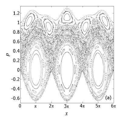
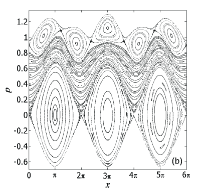
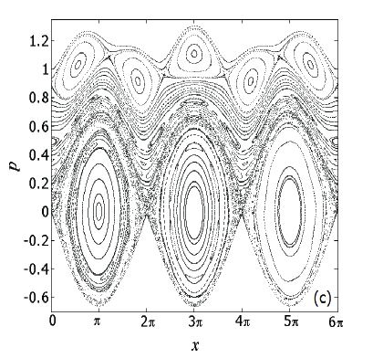
Figure 2: Poincaré sections of Hamiltonian (13) for $s=0.85$ without control term (panel (a)), plus the exact control term (15) (panel (b)) and plus the approximate control term  (16)(panel (c)).

Poincaré sections of Hamiltonian (13) computed for two values of the Chirikov parameter, $s=0.85$ and $s=1.27$, are depicted in Figs. 2-3, panels (a). We notice that in both cases no rotational invariant tori survive and therefore trajectories can diffuse over the whole phase space in between the two primary resonances.

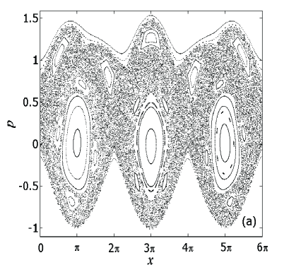
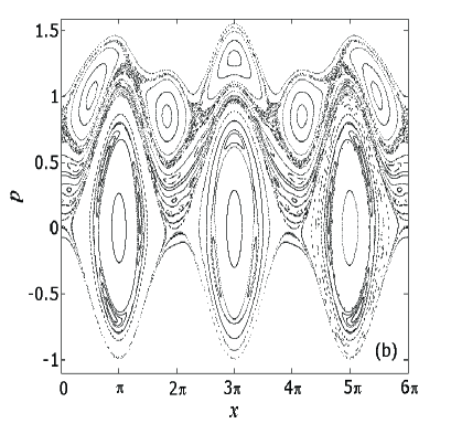
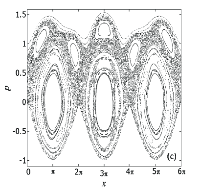
Figure 3: Poincaré sections of Hamiltonian (13) for $s=1.27$ without control term (panel (a)), plus the exact control term (15) (panel (b)) and plus the approximate control term (16) (panel (c)).

As expected, when the exact control term given by Eq. (15) is added to the original Hamiltonian, then rotational invariant tori are restored. This is shown by the two Poincaré sections in Figs. 2 and  3, panels (b), corresponding to the two values $s=0.85$ and $s=1.27$ of the Chirikov parameter. We notice that $s=1.27$ corresponds to a chaotic regime where the two resonances overlap according to Chirikov criterion ($s\geq 1$). Nevertheless the exact control term is able to reconstruct the invariant torus predicted by the method and to regularize a quite large region around the recreated invariant torus.

In order to study the effect of a simplified control term on the electron beam dynamics we perform numerical simulations adding the control term given by Eq. (16) to Hamiltonian (13). As one can see from the Poincaré section depicted in Fig. 2, panels (c), the effect of the approximate control term is still present with the recreation of a set of invariant tori for $s=0.85$. However, this regularization apparently disappears when we consider the fully chaotic regime with $s=1.27$ (see Fig. 3, panel (c)). Nevertheless the approximate control term has still a significant effect on the reduction of chaotic diffusion. This fact can be observed on the probability distribution functions of the electron beam velocity. This diagnostic will also be used in the experiment in order to see the effect of the control terms.

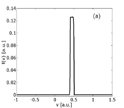
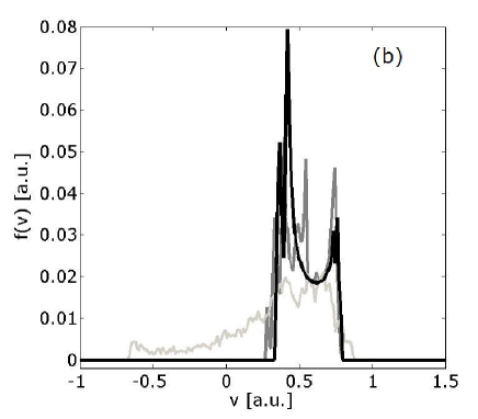
Figure 4: (a): initial beam velocity distribution function for $s=0.85$. (b): final beam velocity distribution function without control term (9) (light gray line), with the exact control term (black line) and with the approximate control term (16)(dark gray line).

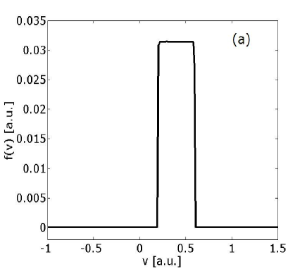
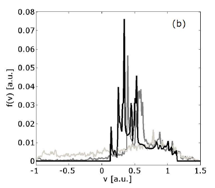
Figure 5: (a): initial beam velocity distribution function for $s=1.27$. (b): final beam velocity distribution function without control term (9) (light gray line), with the exact control term (black line) and with the approximate control term (16) (dark gray line).

In Figs. 4 and  5, the initial velocity distribution function of a set of $10^{4}$ particles is compared with the final one obtained by integrating over a time $t=50$, the dynamics governed by Hamiltonian (13) without control terms, plus the exact control term (15) and plus the approximate control term (16). This investigation is performed for the two different values of the Chirikov parameter, $s=0.85$ for Fig. 4 and $s=1.27$ for Fig. 5. In the case without any control term the original kinetic coherence of the beam is lost which means that some electrons can have velocities in the whole range in between resonances, $v\in[-0.67,0.88]$. Adding the exact control term the particles are confined in a selected region of phase space by the reconstructed invariant tori, and the beam recovers a large part of its initial kinetic coherence. For $s=0.85$, velocities of the electrons are now between $0.33$ and $0.79$. The exact control term is also efficient in the fully chaotic regime ($s=1.27$). Concerning the approximate control term it is very efficient for $s=0.85$ while its efficiency is smaller in the strongly chaotic regime. However, it has still some regularizing effect, inducing the reconstruction of stable islands in phase space which can catch and thus confine a portion of the initial beam particles.

II.4 Robustness of the method

The robustness of the control method for the case $s=1.27$ is studied with respect to an error on the phase or on the amplitude of the computed control term. In experiment, given the frequency $\omega_{1}+\omega_{2}$, the wave number $k_{1}+k_{2}$ of the control term does not satisfy in general the dispersion relation $k=K(\omega)$ since the dispersion relation is not linear. In our case it means that the experimentally implemented control term is not the exact one. For this reason we investigate the robustness of the control term given by Eq. (16) with a phase error $\varphi$, that is

$$f(x,t)=2\varepsilon^{2}r\cos[(k+1)x-kt+\varphi],$$ (17)

and with an error on its amplitude ruled by a factor $\delta$, that is

$$f(x,t)=2\varepsilon^{2}r\delta\cos[(k+1)x-kt].$$ (18)

The values given by Eq. (16) are $\varphi=0$ and $\delta=1$. In order to quantify the robustness of the approximate control term given by Eq. (17) or Eq. (18), we introduce the kinetic coherence indicator defined as the ratio of the variance of the initial beam over the variance of the distribution function after a given integration time. The number of particles, the integration time and the initial conditions are equal to the ones used in the previous section.

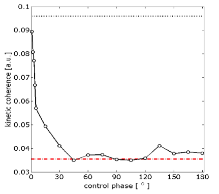
Figure 6: Kinetic coherence versus the phase introduced in the approximate control term given by Eq. (17). The red dash-dotted line indicates the kinetic coherence value for the non-controlled case and the dotted line the kinetic coherence value for the approximate control term. The overlap parameter is $s=1.27$.

In Fig. 6 we show the kinetic coherence as a function of the phase of the approximate control term for the strongly chaotic regime $s=1.27$. We notice that $\varphi$ or $-\varphi$ will give the same velocity distribution function for symmetry reason. Therefore we only consider the range $\varphi\in[0,\pi]$. The efficiency of the approximated control term is very sensitive with respect to the phase. In fact an error of $5^{\mathrm{o}}-6^{\mathrm{o}}$ causes a decrease of the kinetic coherence of about $50\%$ and with an error greater than $30^{\mathrm{o}}$ the kinetic coherence drops in the range of values of the non-controlled case.

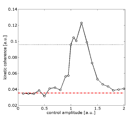
Figure 7: Kinetic coherence versus $\delta$ for the approximate control term given by Eq. (18). The red dash-dotted line indicates the kinetic coherence value for the non-controlled case and the dotted line the kinetic coherence value for the approximate control term given by Eq. (16).The overlap parameter is $s=1.27$.

Concerning the robustness with respect to an error on the amplitude of the approximate control term, we plot on Fig. 7 the behavior of the kinetic coherence as a function of the $\delta$-factor which multiplies the amplitude of the approximate control term. We notice that around the reference value of $\delta=1$ (no error) there is a region ($\delta\in[1,1.3]$) where the approximate control term is very efficient in confining the beam of test particles with a kinetic coherence in between $[0.096,0.12]$. On the other hand reducing the amplitude of the control term, i.e. its energy, there is a region where one has still a confining effect on the beam particle. For example for $\delta=0.6$ the kinetic coherence is larger by $50\%$ of the value of the non-controlled case.

III Experimental tests

III.1 Experimental set-up

The experimental implementation of the control term is performed in a long traveling wave tube (TWT) Pierce ; Gilmour extensively used to mimic beam plasma interaction Tsunoda ; Dimonte and recently to observe resonance overlap responsible for Hamiltonian chaos  Macor1 . The TWT sketched in Fig. 8 is made up of three main elements: an electron gun, a slow wave structure (SWS) formed by a helix with axially movable antennas, and an electron velocity analyzer. The electron gun creates a beam which propagates along the axis of the SWS and is confined by a strong axial magnetic field with a typical amplitude of $0.05{\,\rm T}$ which does not affect the axial motion of the electrons. The central part of the gun consists of the grid-cathode subassembly of a ceramic microwave triode and the anode is replaced by a Cu plate with an on-axis hole whose aperture defines the beam diameter equal to $1{\,\rm mm}$. Beam currents, $I_{b}<1{\,\rm mA}$, and maximal cathode voltages, $|V_{c}|<200{\,\rm V}$, can be set independently; an example of typical velocity distribution functions is given in Figs. 9 and 10 (panel (a)). Two correction coils provide perpendicular magnetic fields to control the tilt of the electron beam with respect to the axis of the helix. For the data shown in this article $I_{b}$ is chosen weak enough to ensure that the beam induces no wave growth and the beam electrons can be considered as test electrons. The SWS is long enough to allow nonlinear processes to develop. It consists in a wire helix that is rigidly held together by three threaded alumina rods and is enclosed by a glass vacuum tube. The pressure at the ion pumps on both ends of the device is $2\times 10^{-9}{\,\rm Torr}$. The $4{\,\rm meter}$ long helix is made of a $0.3{\,\rm mm}$ diameter Be-Cu wire; its radius is equal to $11.3{\,\rm mm}$ and its pitch to $0.8{\,\rm mm}$. A resistive rf termination at each end of the helix reduces reflections. The maximal voltage standing wave ratio is 1.2 due to residual end reflections and irregularities of the helix. The glass vacuum jacket is enclosed by an axially slotted $57.5{\,\rm mm}$ radius cylinder that defines the rf ground. Inside this cylinder but outside the vacuum jacket are four axially movable antennas which are capacitively coupled to the helix and can excite or detect helix modes in the frequency range from 5 to 95  MHz. Only the helix modes are launched, since empty waveguide modes can only propagate above $2{\,\rm GHz}$. These modes have electric field components along the helix axis  Dimonte . Launched electromagnetic waves travel along the helix with the speed of light; their phase velocities, ${v_{\phi j}}$, along the axis of the helix are smaller by approximately the tangent of the pitch angle, giving $2.8\times 10^{6}{\,\rm m/s}<{v_{\phi j}}<5.3\times 10^{6}{\,\rm m/s}$. Waves on the beamless helix are slightly damped, with $|{k_{j}^{0i}}|/|{k_{j}^{0r}}|\approx 0.005$ where ${k^{0}=k^{0r}+{\rm i\,}k^{0i}}$ is the beamless complex wave number. The dispersion relation closely resembles that of a finite radius, finite temperature plasma, but, unlike a plasma, the helix does not introduce appreciable noise. Finally the cumulative changes of the electron beam distribution are measured with the velocity analyzer, located at the end of the interaction region. This trochoidal analyzer guyomarc'h works on the principle that electrons undergo an ${\bf E\times B}$ drift when passing through a region in which an electric field ${\bf E}$ is perpendicular to a magnetic field ${\bf B}$. A small fraction (0.5%) of the electrons passes through a hole in the center of the front collector, and is slowed down by three retarding electrodes. Then the electrons having the correct drift energy determined by the potential difference on two parallel deflector plates are collected after passing through an off-axis hole at the back of the analyzer. The time averaged collected current is measured by means of a pico-ampermeter. Retarding potential and measured current are computer controlled, allowing an easy acquisition and treatment with an energy resolution lower than $0.5{\,\rm eV}$. In the absence of any emitted wave, after propagating along the helix, the beam exhibits a sharp velocity distribution function with a velocity width mainly limited by the analyzer resolution as shown in Figs. 9 and 10 (panel (a)). For Fig. 9a, the beam with radius 3mm is diffracted by passing through the three grounded grids of a spreader spreader just after leaving the gun while for Fig. 10a, the beam radius is $1{\,\rm mm}$ and the spreader has beem removed for the sake of simplicity.

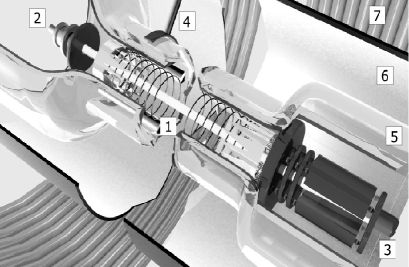
Figure 8: Sketch of the Travelling Wave Tube: (1) helix, (2) electron gun, (3) trochoidal analyzer, (4) antenna, (5) glass vacuum tube, (6) slotted rf ground cylinder, and (7) magnetic coil.

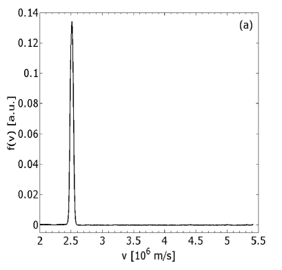
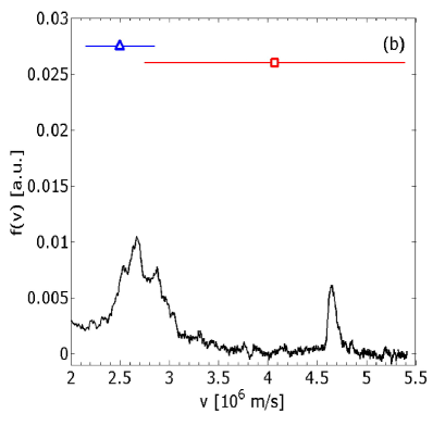
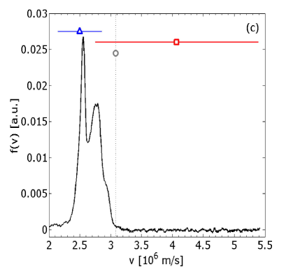
Figure 9: Beam velocity distribution functions at the output of the TWT for $s=0.85$ : (a) test beam ($I_{b}=50$ nA) without electrostatic wave, (b) with helix mode (trapping domain shown by red line with phase velocity marked by a square) and beam mode (trapping domain shown by blue line with phase velocity marked by a triangle) at 30 MHz , (c) with an additional controlling wave at $60$ MHz and phase velocity given by grey circle and dotted line.

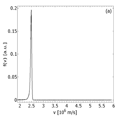
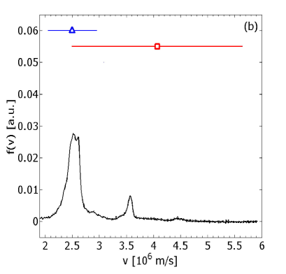
Figure 10: Beam velocity distribution functions at the output of the TWT for $s=1.27$ : (a) test beam ($I_{b}=2$ nA) without electrostatic wave, (b) with helix mode (trapping domain shown by red line with phase velocity marked by a square) and beam mode (trapping domain shown by blue line with phase velocity marked by a triangle) at 30 MHz, (c) with an additional controlling wave at $60$ MHz and phase velocity given by grey circle and dotted line.

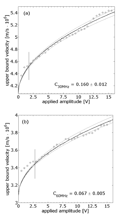
Figure 11: Measure of helix mode coupling constant $C_{h}$ calculated from the measured upper bound velocity of trapping domain (circles) at frequency $f$ equal to (a) 30 MHz and (b) 60 MHz. Black line parabola is obtained using the average value of $C_{h}$. Gray parabolas are given by the average error. The parabolic fit is only valid beyond the vertical segment indicating the wave amplitude beyond which beam trapping occurs over the length of the TWT.

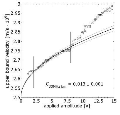
Figure 12: Measure of coupling constant $C_{b}$, at frequency equal to 30 MHz for a beam mode at $2.5\times 10^{6}$ m/s. Black line parabola is obtained using the average value of $C_{b}$, calculated from the upper bound velocity of the trapping domain between the vertical segments where the beam become trapped over the length of the TWT and the ”devil’s staircase” is not yet evident escalier . Two independent measures are shown by circles and squares to give an error estimate.

.

III.2 Experimental implementation of the control term

We apply an oscillating signal at the frequency of 30 MHz on one antenna. It generates two waves: a helix mode with a phase velocity equal to $v_{\varphi}=4.07\times 10^{6}$ m/s, a beam mode with a phase velocity equal to the beam velocity $v_{b}$ (in fact two modes with pulsation $\omega=kv_{b}\pm\omega_{b}$ corresponding to the beam plasma mode with pulsation $\omega_{b}=(n_{b}e^{2}/m\epsilon_{0})^{1/2}$, Doppler shifted by the beam velocity $v_{b}$, merging in a single mode since $\omega_{b}\ll\omega$ in our conditions). Figures 9 and 10 (panel (b)) show the measured velocity distributions of the beam after interacting with these two modes over the length of the TWT for two different values of the Chirikov parameter. The case with $s=0.85$ was previously investigated  c18 . The red square (resp. blue triangle) shows the phase velocity $v_{\varphi}$ (resp.$v_{b}$) of the helix (resp. beam) mode on the middle of the resonant domain determined as the trapping velocity width of the helix mode $v_{\varphi}\pm 2\sqrt{eC_{h}\Phi/m}$ (resp. $v_{b}\pm 2\sqrt{eC_{b}\Phi/m}$ ) where $\Phi$ is the signal amplitude applied on the antenna and $C_{h}\Phi=3542{\rm mV}$ (resp. $C_{b}\Phi=286{\rm mV}$) is the real amplitude of the helix (resp. beam) mode. Both $C_{h}$ and $C_{b}$ are determined experimentally by the estimations of the coupling constant for helix $C_{h}$(resp. beam $C_{b}$) mode. As shown in Fig. 11 the helix mode coupling coefficient $C_{h}$ is obtained by fitting a parabola through the measured upper bound velocity (circles) after the cold test beam with initial velocity equal to the wave phase velocity has been trapped by the wave at a given frequency over the total length of the TWT. As shown in Fig. 12, the beam mode coupling coefficient $C_{b}$ is obtained by fitting a parabola through the measured upper bound velocity (circles) for a beam with a mean velocity very different from the helix mode phase velocity at the considered frequency. These two domains overlap and the break up of invariant KAM tori (or barriers to velocity diffusion) results in a large spread of the initially narrow beam of Figs. 9 and 10 (panel (b)) over the chaotic region  Macor1 . We now use an arbitrary waveform generator Tsunoda to launch the same signal at $30$ MHz and an additional control wave with frequency equal to $60$ MHz, an amplitude and a phase given by Eq. (11). The beam velocity is also chosen in such a way that the wave number of the helix mode at 60 MHz properly satisfies the dispersion relation function shown as circles in Fig. 1. We neglect the influence of the beam mode at $60$ MHz since its amplitude is at least an order of magnitude smaller than the control amplitude as shown by comparing Figs.  11a and  12 for $30$ MHz. As observed on Figs. 9 and 10(panel (c)) where the grey circle indicates the phase velocity of the controlling wave, the beam recovers a large part of its initial kinetic coherence. For $s=0.85$ (see Fig. 9c) the beam does not spread in velocity beyond the reconstructed KAM tori, in agreement with the numerical simulations of Fig. 2. For the more chaotic regime (see Fig. 10b) with $s=1.27$ the improvement of the kinetic coherence is still present as shown in Fig. 10c. It can no more be associated with the reconstruction of a local velocity barrier, as expected from the numerical results in Fig. 3 (panel (c)). For this last overlap parameter an experimental exploration of the robustness of the method will be shown in the next section.

III.3 Robustness of the method

In our experiment the control term is given by an additional wave whose frequency, amplitude and phase are computed as shown in Sec. II. In order to quantify the robustness of the method we will compare the various experimental situations to a reference one (Fig. 10a). This reference is taken as the (initial) cold beam distribution function. An example of the distribution we were able to reach with control is given in Fig. 10c. The control amplitude is $140$ mV in agreement with $144$ mV given by the method up to experimental errors. The phase is chosen experimentally and arbitrarily labelled $0^{\rm o}$. The beam velocity is chosen equal to $2.498\times 10^{6}$ m/s in agreement with $2.51\times 10^{6}$ m/s as estimated from the dispersion relation shown in Fig. 1.

We investigate the robustness of the control method with respect to variation of phase and amplitude in the approximate control term given by Eq. (11).

We use the kinetic coherence indicator to quantify the effect of the control, defined as the ratio of variance of the cold beam distribution function over the variance of the distribution function. Other indicators (integral and uniform distances) were used and gave similar results. Figure 13 shows the velocity distribution functions for two values of the phase ($-5^{\rm o}$ and $22.5^{\rm o}$) keeping the other parameters constant. It shows that for a phase equal to $-5^{\rm o}$ close to the reference value the two velocity distribution functions are very similar, and more peaked at $-5^{\rm o}$ than at $0^{\rm o}$. For $22.5^{\rm o}$, the control wave has the opposite effect, increasing chaos. In Fig. 14 we show the kinetic coherence as a function of the phase of the approximate control term. It shows a narrow region around the reference value where the control wave is the most efficient.

In Fig. 15, we represent the kinetic coherence as a function of the amplitude of the control wave. When changing the control wave amplitude a resonance condition in a narrow region around the optimized amplitude is still observed. For amplitudes smaller than the reference (computed) value the effect of the control decays fast and the electron velocities are more widely spread than in the non-controlled case. Besides, for larger values, the beam velocity spread increases but the control term energy becomes comparable to the beam mode energy changing radically the initial system. We have observed, due to beam current conservation, a lower peak at initial beam velocity implies that electron velocities are more widely spread. An enlargement of distribution around the main peak is shown in Figs. 16 a,b and confirms that $140$ mV appears to be the optimum.

Finally we check the sensitivity of the control mode with respect to the initial beam velocity. This corresponds introducing an error both on the wave number and on the amplitude of the control mode. The overlap parameter $s$ depends on the phase velocity difference between the helix and beam modes (see Eq.( 2)); for such a reason we also measure the non-controlled velocity distribution function for each initial beam velocity. Figure 17a clearly exhibits the resonant condition expected at the reference value $2.51\times 10^{6}$ m/s. We also note that, without control, chaos is continuously increasing as expected since when the phase velocity difference decreases resonance overlap (and chaos) increases. Figure 18 shows how two beams with close initial velocities with similar chaotic behavior have two different responses to the same control term.

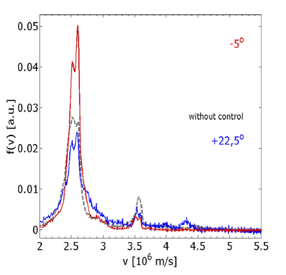
Figure 13: Distribution functions for the maximum kinetic coherence value (resp. minimum), blue line (resp. red line), is compared with the non-controlled distribution function (grey dashed line). The overlap parameter is $s=1.27$.

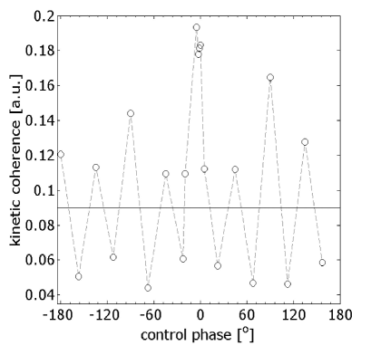
Figure 14: Kinetic coherence defined as the variance of the cold beam distribution function over the variance of distribution function for different control term phases, an optimized amplitude $140$ mV and a beam velocity $2.498\times 10^{6}$ m/s. Control becomes efficient in a narrow region close to zero. Solid line shows the level of the kinetic coherence for the non-controlled case. Dashed line is only an eye-guide. The overlap parameter is $s=1.27$.

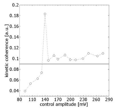
Figure 15: Kinetic coherence defined such as in Fig. 14a for different control amplitudes and a phase $0^{\rm o}$ and a beam velocity $2.498\times 10^{6}$  m/s. Control becomes efficient in a narrow region around $140$  mV. Solid line shows the level of the kinetic coherence for the non-controlled chaos. Dashed line is only an eye-guide. The overlap parameter is $s=1.27$.

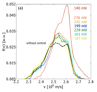
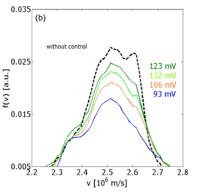
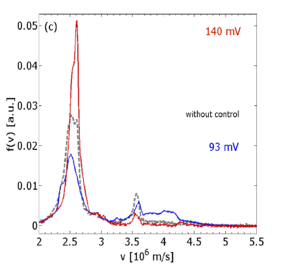
Figure 16: Enlargement of velocity distribution functions close to initial beam velocity for different control amplitudes: (a) larger, (b) lower than experimentally optimized amplitude $140$  mV. (c) velocity distribution functions for three different control amplitudes at fixed control phase equal to $0^{\rm{o}}$. The overlap parameter is $s=1.27$.

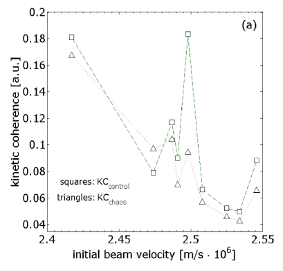
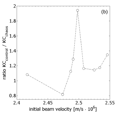
Figure 17: Kinetic coherence versus initial beam velocity with optimized control term amplitude ($140$ mV) and phase ($0^{\rm o}$). (a), squares (resp. triangles) show the values for velocity distribution function obtained with (resp. without) applied control term. (b), Ratio between kinetic coherence measured with and without control for different initial beam velocity. The overlap parameter is $s=1.27$.

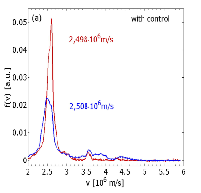
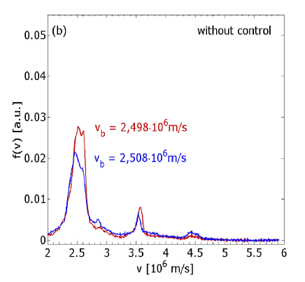
Figure 18: Velocity distribution functions for two close values of initial beam velocity (a) with and (b) without applied control . The overlap parameter is $s=1.27$.

IV Summary and conclusion

Even if a modification of the perturbation of a Hamiltonian system generically leads to the enhancement of the chaotic behavior, we have applied numerically and experimentally a general strategy and an explicit algorithm to design a small but apt modification of the potential which drastically reduces chaos and its attendant diffusion by channeling chaotic transport. The experimental results show that the method is tractable and robust, therefore constituting a natural way to control the dynamics. The robustness of the method has been checked for an overlap parameter equal to $s=1.27$ by changing phase and amplitude of the control term and beam velocity to check resonance condition on the helix dispersion relation. All these measurements have shown a significant region around the prescribed values for which the control is efficient. The implementation is realized with an additional cost of energy which corresponds to less than $1\%$ of the initial energy of the two-wave system. We stress the importance of a fine tuning of the parameters of the theoretically computed control term (e.g., amplitude, phase velocity) in order to force the experiment to operate in a more regular regime. For such a reason an iterative process to find some optimal experimental conditions is suggested for future improvement of the method. Other control terms can be used to increase stability (by taking into account the other Fourier modes of $f$ given in Eq. (9) when experimentally feasible). The achievement of control and all the tests on a TWT assert the possibility to practically control a wide range of systems at a low additional cost of energy.

V Acknowledgment

A.M. and F.D. are grateful to J-C. Chezeaux, D. Guyomarc’h, and B. Squizzaro for their skillful technical assistance, and to D.F. Escande and Y. Elskens for fruitful discussions and a critical reading of the manuscript. A. M. benefits from a grant by Ministère de la Recherche. This work is partially supported by Euratom/CEA (contract EUR 344-88-1 FUA F).

References

- (1) A.J. Lichtenberg and M.A. Lieberman, Regular and Chaotic Dynamics (Springer, New York, 1992).
- (2) L.P. Kadanoff, From Order to Chaos: Essays : Critical, Chaotic and Otherwise, vol. I (1993) and II (1998) (World Scientific, Singapore).
- (3) G. Chen and X. Dong, From Chaos to Order (World Scientific, Singapore, 1998).
- (4) D.J. Gauthier, Controlling chaos, Am. J. Phys. 71, 750 (2003).
- (5) W.L. Ditto, S.N. Rauseo and M.L. Spano, Experimental control of chaos, Phys. Rev. Lett. 65, 3211 (1990).
- (6) V. Petrov, V. Gaspar, J. Masere and K. Showalter, Controlling chaos in the Belousov-Zhabotinsky reaction, Nature 361, 240 (1993).
- (7) S.J. Schiff et al., Controlling chaos in the brain, Nature 370, 615 (1994).
- (8) Y. Braiman, J.F. Lindner and W.L. Ditto, Taming spatiotemporal chaos with disorder, Nature 378, 465 (1995).
- (9) L.S. Pontryagin, V.G. Boltyanskii, R.V. Gamkrelidze and E.F. Mishchenko, The mathematical theory of optimal processes (Wiley, New York, 1961).
- (10) E. Ott, C. Grebogi and J.A. Yorke, Controlling chaos, Phys. Rev. Lett. 64, 1196 (1990).
- (11) R. Lima and M. Pettini, Suppression of chaos by resonant parametric perturbations, Phys. Rev. A 41, 726 (1990).
- (12) T. Shinbrot, C. Grebogi, E. Ott and J.A. Yorke, Using small perturbations to control chaos, Nature 363, 411 (1993).
- (13) E. Ott and M. Spano, Controlling chaos, Phys. Today 48, 34 (1995).
- (14) R.D. Hazeltine and S.C. Prager, New physics in fusion plasma confinement, Phys. Today 55, 30 (2002).
- (15) C. Chandre, M. Vittot, G. Ciraolo, Ph. Ghendrih and R. Lima, Control of stochasticity in magnetic field lines, Nuclear Fusion 46, 33 (2006).
- (16) Y. Elskens and D.F. Escande, Microscopic Dynamics of Plasmas and Chaos (IoP Publishing, Bristol, 2003).
- (17) B.V. Chirikov, A universal instability of many-dimensional oscillator systems, Phys. Rep. 52, 263 (1979).
- (18) F. Doveil, Kh. Auhmani, A. Macor and D. Guyomarc’h, Experimental observation of resonance overlap responsible for Hamiltonian chaos, Phys. Plasmas 12, 010702 (2005).
- (19) C. Chandre, G. Ciraolo, F. Doveil, R. Lima, A. Macor and M. Vittot, Channeling Chaos by Building Barriers, Phys. Rev. Lett 94, 074101 (2005).
- (20) J.R. Pierce, Travelling wave tubes (Van Nostrand, Princeton, 1950).
- (21) A.S. Gilmour Jr., Principles of travelling wave tubes (Artech House, London, 1994).
- (22) S.I. Tsunoda, F. Doveil and J.H. Malmberg, Experimental test of the quasilinear theory of the interaction between a weak warm electron beam and a spectrum of waves, Phys. Rev. Lett. 58, 1112 (1987).
- (23) G. Dimonte and J.H. Malmberg, Destruction of trapping oscillations, Phys. Fluids 21, 1188 (1978).
- (24) D. Guyomarc’h and F. Doveil, A trochoidal analyzer to mesure the electron beam energy distribution in a traveling wave tube, Rev. Sci. Instrum. 71, 4087 (2000).
- (25) F. Doveil, S.I. Tsunoda and J.H.Marlberg, Controlled production of warm electron beams, Rev. Sci. Instrum. 67, 2157 (1996).
- (26) A. Macor, F. Doveil and Y. Elskens, Electrons climbing a ”devil’s staircase” in wave-particle interaction, Phys. Rev. Lett. 95, 264102 (2005).