Maxwell’s demon through the looking glass

Abstract

Mechanical Maxwell’s demons, such as Smoluchowski’s trapdoor and Feynman’s ratchet and pawl need external energy source to operate. If you cease to feed a demon the Second Law of thermodynamics will quickly stop its operation. Nevertheless, if the parity is an unbroken symmetry of nature, it may happen that a small modification leads to demons which do not need feeding. Such demons can act like perpetuum mobiles of the second kind: extract heat energy from only one reservoir, use it to do work and be isolated from the rest of ordinary world. Yet the Second Law is not violated because the demons pay their entropy cost in the hidden (mirror) sector of the world by emitting mirror photons.

I Introduction

“The law that entropy always increases - the second law of thermodynamics - holds, I think, the supreme position among the laws of nature. If someone points out that your pet theory of the universe is in disagreement with Maxwell’s equations - then so much the worse for Maxwell’s equations. If it is found to be contradicted by experiments - well, these experimentalists do bungle things sometimes. But if your theory is found to be against the second law of thermodynamics I can give you no hope; there is nothing for it but to collapse in deepest humiliation” 1 . Following Eddington’s this wise advice, I will not challenge the Second Law in this article. Demonic devices I consider are by no means malignant to the Second Law and their purpose is not to oppose it but rather to demonstrate possible subtleties of the Law’s realization in concrete situations.

This philosophy is much in accord with Maxwell’s original intention who introduced “a very observant and neat-fingered being”, the Demon, as a means to circumscribe the domain of validity of the Second law and in particular to indicate its statistical nature 2 ; 3 ; 4 .

Later, however, it became traditional to consider demons as a threat to the Second Law to be defied. Modern exorcisms use information theory language and it is generally accepted that the Landauer’s principle 5 ; 6 ; 7 finally killed the demon.

But, as Maxwell’s demon was considered to be killed several times in the past and every time it resurrected from dead, we have every reason to suspect this last information theory exorcism 3 ; 8 ; 9 and believe the old wisdom that “True demons cannot be killed at all” 10 .

The problem with all exorcisms can be formulated as a dilemma 8 : either the whole combined system the demon included forms a canonical thermal system or it does not. In the first case the validity of the Second Law is assumed from the beginning and therefore the demon is predefined to fail. The exorcism is sound but not profound, although sometimes it can be enlightening and delightful.

In the second case it is not evident at all why anti-entropic behaviour can not happen. For example, if Hamiltonian dynamics is abandoned, a pressure demon can readily be constructed 11 . One needs a new physical postulate with independent justification to ensure the validity of the Second Law for the combined system. Although Landauer’s principle can be proved in several physical situations 12 ; 13 its generality is not sufficient to exorcise all conceivable extraordinary demons. For example, the Landauer’s principle, as well as ordinary Gibbsian thermodynamics, fails in the extreme quantum limit then the entanglement is essential and the total entropy is not the sum of partial entropies of the subsystems 14 .

According to Boltzmann, “The second law of thermodynamics can be proved from the mechanical theory if one assumes that the present state of the universe, or at least that part which surrounds us, started to evolve from an improbable state and is still in a relatively improbable state. This is a reasonable assumption to make, since it enables us to explain the facts of experience, and one should not expect to be able to deduce it from anything more fundamental” 15 . But how improbable? Roger Penrose estimates 15 ; 16 that the initial state of the universe was absurdly improbable: one part in $10^{10^{123}}$. In the face of this number, I think, you would rather welcome Maxwell’s demon than want to exorcise it. Of course, recent approaches to the Low Entropy Past problem 17 do not involve demons, but who can guarantee that the initial low entropy state was prepared without them? In any case something more fundamental is clearly required to explain the puzzle and avoid sheer impossibility of the world we observe around us.

It seems, therefore, that exorcism is not productive and it is better to allow the presence of demons. However the notion of demons should be understood in broader sense: not only creatures which challenge the Second Law, but also the ones which use the Second Law in a clever and rather unexpected manner.

The rest of the paper is organized as follows. In the first sections we consider some classical Maxwell demons. A rather detailed analysis of them is presented in the framework of the Langevin and Fokker-Planck equations. I tried to make the exposition as self-contained as possible, assuming that readers from the mirror matter community are as unfamiliar with some subtleties of the Fokker-Planck equation, like Itô-Stratonovich dilemma, as was the author months ago.

After demonstrating that the demons really work when the temperature difference between their two thermal baths is enforced, we speculate about a possibility that this temperature difference can be naturally created if significant amount of mirror matter is added to one of the thermal reservoirs.

Mirror matter is a hypothetical form of matter expected to exist if nature is left-right symmetric in spite of P and CP violations in weak interactions. An example from the molecular physics is considered to support this possibility. We cite some review articles where more detailed and traditional exposition of the mirror matter idea, as well as relevant references, can be found.

The conclusion just finishes the paper with the cheerful remark that mirror matter demons might be technologically very useful. Therefore it is worthwhile to search mirror matter experimentally. It is remarked that one experiment which searches invisible decays of orthopositronium in vacuum is under way.

II Smoluchowski’s trapdoor

Maxwell’s original demon operates a tiny door between two chambers filled with gas allowing only fast molecules to pass in one direction, and only slow ones to pass in opposite direction. Eventually a temperature difference is generated between the chambers. The demon can be just some purely mechanical device to avoid complications connected with the demon’s intellect and information processing. If this device is assumed to be subject of conventional thermodynamics (the sound horn of the dilemma mentioned above) then the demon can succeed only if it hides entropy somewhere else. A very clever way how to do this was indicated recently 18 .

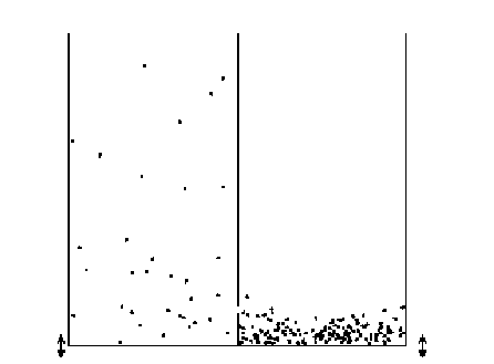
Figure 1: Sand as Maxwell’s Demon 18 .

In Fig.1 Maxwell’s demon left the door between two chambers ajar but this shrewd creature had replaced the molecules in the chambers by sand grains and set the chambers in vertical vibration by mounting them on a shaker. Usually sand grains distribute equally to both sides. But if the vibration frequency is lowered below a critical value something remarkable happens: the symmetry is spontaneously broken and grains settle preferentially on one side. The sand grains act as a Maxwell’s demon! This is possible because, in contrast to a molecular gas, collisions between grains of sand are not elastic and grains are simply heated during the collisions, absorbing the entropy 18 .

One of the oldest mechanical Maxwell’s demon is the Smoluchowski’s trapdoor 19 . Two chambers filled with gas are connected by an opening that is covered by a spring-loaded trapdoor. Molecules from one side tend to push the door open and those on the other side tend to push it closed. Naively one expects that this asymmetry in the construction of the door turns it into a one-way valve which creates a pressure difference between the chambers.

Smoluchowski argued that the thermal fluctuations of the door will spoil the naive picture and prohibit it to act as a one-way valve, although he did not provide detailed calculations to prove this fact conclusively. It is difficult to trace the trapdoor demon analytically to see how it fails, but the corresponding computer simulations can be done and the results show that Smoluchowski was right 19 ; 20 .

The simulations show that the pressure difference between the chambers is exactly what is expected at equilibrium after the trapdoor’s finite volume is taken into account. Therefore the trapdoor can not act as a pressure demon.

But if the trapdoor is cooled to reduce its thermal fluctuations the demon becomes successful and indeed creates a measurable pressure difference between the chambers. In simulation program the effective cooling of the door is maintained by periodically removing energy from the door then it is near the central partition. As a result the door remains near the closed position longer than would occur without the cooling and it indeed operates as a one-way valve 19 ; 20 .

The entropy decrease due to this pressure demon is counterbalanced by the entropy increase in the refrigerator that cools the door below the ambient gas temperature. However the demonstration of this fact in computer simulations involves some subtleties 20 .

III Feynman’s ratchet and pawl

Close in spirit to the Smoluchowski’s trapdoor is Feynman’s ratchet and pawl mechanism 21 . The device (Fig.2) contains a box with some gas and an axle with vanes in it. At the other end of the axle, outside the box, there is toothed wheel and a pawl that pushes on the cogwheel through a spring.

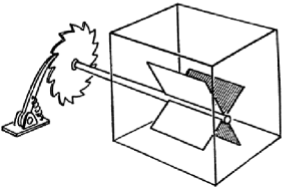
Figure 2: Feynman’s ratchet and pawl engine 21 .

If the paddle wheel is small enough, collisions of gas molecules on the vanes will lead to Brownian fluctuations of the axle. But the ratchet on the other end side of the axle allows rotation only in one direction and blocks the counter-rotation. Therefore one expects Feynman’s ratchet and pawl engine to rectify the thermal fluctuations in a similar manner as the use of ratchets allow windmills to extract useful work from random winds.

At closer look, however, we realize that the miniature pawl would itself be subject to thermal fluctuations that invalidate its rectification property. In isothermal conditions, when the vanes have the same temperature as the ratchet and pawl, the Second Law ensures that the rate of rotations in a wrong direction due to the pawl’s thermal bounces just compensates the rate of the favorable rotations so that the wheel does a lot of jiggling but no net turning. However if the temperatures are different the rate balance no more holds and the ratchet and pawl engine really begins to rotate 21 ; 22 ; 23 ; 24 .

Yet there are some subtleties and by way of proof it is better to go into some details by modeling the ratchet and pawl machine by the following Langevin equations 25 :

$$\lambda\frac{d\theta_{1}}{dt}=F(\theta_{1})-k(\theta_{1}-\theta_{2})+f_{1}(t),$$

$$\lambda\frac{d\theta_{2}}{dt}=k(\theta_{1}-\theta_{2})+f_{2}(t),$$ (1)

where $\theta_{1}$ and $\theta_{2}$ are the angular positions of the ratchet and the windmill respectively, $\lambda$ is the friction coefficient assumed to be the same for both baths, $F(\theta_{1})=-\frac{\partial U}{\partial\theta_{1}}$ is the torque the ratchet experiences due to an asymmetric potential $U(\theta_{1})$ of its interaction with the pawl. It is assumed that the ratchet and the windmill are connected by an elastic spring of rigidity $k$. Finally, $f_{1}(t)$ and $f_{2}(t)$ represent Brownian random torques on the ratchet and on the windmill respectively due to thermal fluctuations. It is assumed that these random torques constitute two independent Gaussian white noises

$$<f_{i}(t)>=0,\;\;\;<f_{i}(t)\,f_{j}(t^{\prime})>=2k_{B}T_{i}\lambda\,\delta_{ij}\,\delta(t-t^{\prime}),$$ (2)

$k_{B}$ being the Boltzmann constant. These Langevin equations correspond to the over-dumped regime (with neglected inertia).

It is more convenient to introduce another set of angular variables

$$\Theta=\frac{1}{2}(\theta_{1}+\theta_{2}),\;\;\;\theta=\frac{1}{2}(\theta_{1}-\theta_{2}).$$ (3)

It is the variable $\Theta$ which describes the net rotation of the system and is, therefore, the only object of our interest, while the variable $\theta$ describes the relative motion and is irrelevant for our goals. In terms of these variables, equations (1) read

$$\lambda\,\dot{\Theta}=\frac{1}{2}F(\Theta+\theta)+\frac{1}{2}\left[f_{1}(t)+f_{2}(t)\right],$$

$$\lambda\,\dot{\theta}=\frac{1}{2}F(\Theta+\theta)-2k\theta+\frac{1}{2}\left[f_{1}(t)-f_{2}(t)\right].$$ (4)

The relative rotation $\theta$ arises due to the Brownian jiggling of the ratchet and of the windmill and hence is expected to be very small. Therefore one can expand

$$F(\Theta+\theta)\approx F(\Theta)+\theta\,F^{\,\prime}(\Theta),\;\;F^{\,\prime}(\Theta)\equiv\frac{dF}{d\Theta}.$$

Besides, the dynamics of the variable $\theta$ is very rapid and at any time scale, relevant for the evolution of the slow variable $\Theta$, the fast variable $\theta$ will be able to relax to a quasi-stationary value given by setting $\dot{\theta}=0$ in the second equation of (4):

$$\theta\approx\frac{F(\Theta)+f_{1}(t)-f_{2}(t)}{4k-F^{\,\prime}(\Theta)}.$$ (5)

This allows to eliminate $\theta$ from (4) and arrive at the following equation for the relevant variable $\Theta$ 25 :

$$\dot{\Theta}=H(\Theta)+g_{1}(\Theta)f_{1}(t)+g_{2}(\Theta)f_{2}(t),$$ (6)

where

$$H(\Theta)=\frac{F(\Theta)}{2\lambda}\left[1+\frac{F^{\,\prime}(\Theta)}{4k}\right],\;\;g_{1}(\Theta)=\frac{1}{2\lambda}\left[1+\frac{F^{\,\prime}(\Theta)}{4k}\right],\;\;g_{2}(\Theta)=\frac{1}{2\lambda}\left[1-\frac{F^{\,\prime}(\Theta)}{4k}\right],$$

and terms of the second and higher order in $\frac{F^{\,\prime}(\Theta)}{4k}$ were neglected.

The resulting Langevin equation (6) is the stochastic differential equation with multiplicative noises and, therefore, subject to the notorious Itô-Stratonovich dilemma 26 ; 27 . The problem is that stochastic integrals one needs to calculate various average values are in general ill-defined without additional interpretation rules (the white noise is a singular object after all, like the Dirac’s $\delta$-function). The most commonly used Itô and Stratonovich interpretations of stochastic integrals lead to different results when multiplicative noise is present.

From the physics side, this ill-definedness may be understood as follows 27 . According to (6) each $\delta$-pulse in $f_{1}(t)$ or $f_{2}(t)$ gives rise to a pulse in $\dot{\Theta}$ and hence an instantaneous jump in $\Theta$. Then it is not clear which value of $\Theta$ should be used in $g_{1}(\Theta)$ and $g_{2}(\Theta)$: the value just before the jump, after the jump, or some average of these two. Itô prescription assumes that the value before the jump should be used, while Stratonovich prescription advocates for the mean value between before and after the jump.

Our manipulations, which led to (6) from (1), already assumes the Stratonovich interpretation because we had transformed variables in (1) as if (1) were ordinary (not stochastic) differential equations and this is only valid for the Stratonovich interpretation 27 .

In fact there is a subtle point here. The naive adiabatic elimination of the fast variable we applied for $\theta$ (by setting $\dot{\theta}=0$) not necessarily implies the Stratonovich interpretation 28 . Depending on the fine details of the physical system and of the limiting process, one may end with Stratonovich, Itô or even with some other interpretation which is neither Itô nor Stratonovich 28 . Nevertheless the Stratonovich interpretation will be assumed in the following like as was done tacitly in 25 .

Let $P(\Theta,t)$ be the probability density for the stochastic process $\Theta(t)$. Then

$$P(\Theta,t)=\int\limits_{-\infty}^{\infty}G(\Theta,t;\,\Theta_{0},t_{0})\,P(\Theta_{0},t_{0})\,d\Theta_{0},\;\;t>t_{0},$$ (7)

where the Green’s function (the conditional probability density over $\Theta$ at time $t$ under the condition that $\Theta=\Theta_{0}$ at $t=t_{0}$) satisfies the initial value equation

$$G(\Theta,t_{0};\,\Theta_{0},t_{0})=\delta(\Theta-\Theta_{0}).$$ (8)

Now consider

$$\frac{\partial P(\Theta,t)}{\partial t}=\lim_{\Delta t\to 0}\frac{P(\Theta,t+\Delta t)-P(\Theta,t)}{\Delta t}.$$ (9)

According to (7)

$$P(\Theta,t+\Delta t)=\int\limits_{-\infty}^{\infty}G(\Theta,t+\Delta t;\,\Theta_{0},t)\,P(\Theta_{0},t)\,d\Theta_{0}.$$ (10)

As the time interval $\Delta t$ is very short, the function $G(\Theta,t+\Delta t;\,\Theta_{0},t)$ can differ from its initial $\delta$-function value only slightly by drifting and broadening a little which can be modeled by the drift coefficient $D^{(1)}(\Theta)$ and the diffusion coefficient $D^{(2)}(\Theta)$ respectively if we expand 29

$$G(\Theta,t+\Delta t;\,\Theta_{0},t)\approx\delta(\Theta-\Theta_{0})+D^{(1)}(\Theta_{0})\,\Delta t\,\delta^{(1)}(\Theta-\Theta_{0})+D^{(2)}(\Theta_{0})\,\Delta t\,\delta^{(2)}(\Theta-\Theta_{0}),$$ (11)

where $\delta^{(n)}(\Theta)$ denotes the $n$-th order derivative of the $\delta$-function with the basic property

$$\int\limits_{-\infty}^{\infty}f(\Theta)\,\delta^{(n)}(\Theta-\Theta_{0})\,d\Theta=\frac{(-1)^{\,n}}{n\,!}\,\left.\frac{d^{\,n}f(\Theta)}{d\Theta^{n}}\right|_{\Theta=\Theta_{0}}.$$

Substituting (11) into (10) we get

$$P(\Theta,t+\Delta t)\approx P(\Theta,t)+\Delta t\,\frac{\partial}{\partial\Theta}\left[D^{(1)}(\Theta)\,P(\Theta,t)\right]+\frac{\Delta t}{2}\,\frac{\partial^{2}}{\partial\Theta^{2}}\left[D^{(2)}(\Theta)\,P(\Theta,t)\right]$$ (12)

and therefore (9) implies the following Fokker-Planck equation

$$\frac{\partial P(\Theta,t)}{\partial t}=\frac{\partial}{\partial\Theta}\left[D^{(1)}(\Theta)\,P(\Theta,t)\right]+\frac{1}{2}\,\frac{\partial^{2}}{\partial\Theta^{2}}\left[D^{(2)}(\Theta)\,P(\Theta,t)\right].$$ (13)

The Fokker-Planck equation determines the evolution of the probability density provided the drift and diffusion coefficient functions are known. These functions are related to the first two moments the initially localized density function develops in the short time interval $\Delta t$ because (12) indicates that

$$<\Delta\Theta>\,=\int\limits_{-\infty}^{\infty}(\Theta-\Theta_{0})\,P(\Theta,t+\Delta t)\,d\Theta=-D^{(1)}(\Theta_{0})\,\Delta t,$$

$$<(\Delta\Theta)^{2}>\,=\int\limits_{-\infty}^{\infty}(\Theta-\Theta_{0})^{2}\,P(\Theta,t+\Delta t)\,d\Theta=D^{(2)}(\Theta_{0})\,\Delta t,$$ (14)

if $P(\Theta,t)=\delta(\Theta-\Theta_{0})$.

On the other hand, these moments can be calculated directly from the Langevin equation. Integrating (6), we get

$$\Delta\Theta=\int\limits_{t}^{t+\Delta t}H(\Theta)\,dt^{\prime}+\int\limits_{t}^{t+\Delta t}g_{1}(\Theta)f_{1}(t^{\prime})\,dt^{\prime}+\int\limits_{t}^{t+\Delta t}g_{2}(\Theta)f_{2}(t^{\prime})\,dt^{\prime}.$$

According to the Stratonovich prescription, in the last two stochastic integrals $\Theta$ should be replaced with

$$\frac{\Theta(t)+\Theta(t+\Delta t)}{2}\approx\Theta(t)+\frac{1}{2}\dot{\Theta}(t)\,\Delta t=\Theta_{0}+\frac{\Delta t}{2}\left[H(\Theta_{0})+g_{1}(\Theta_{0})f_{1}(t)+g_{2}(\Theta_{0})f_{2}(t)\right],$$

where $\Theta_{0}=\Theta(t)$. But

$$g(\Theta_{0}+\Delta\Theta)\approx g(\Theta_{0})+\Delta\Theta\left.\frac{\partial g}{\partial\Theta}\right|_{\Theta=\Theta_{0}}.$$

Therefore we obtain

$$\Delta\Theta\approx H(\Theta_{0})\,\Delta t+\frac{\Delta t}{2}\left[H(\Theta_{0})+g_{1}(\Theta_{0})f_{1}(t)+g_{2}(\Theta_{0})f_{2}(t)\right]\times$$

$$\left[\frac{\partial g_{1}}{\partial\Theta}(\Theta_{0})\int\limits_{t}^{t+\Delta t}f_{1}(t^{\prime})\,dt^{\prime}+\frac{\partial g_{2}}{\partial\Theta}(\Theta_{0})\int\limits_{t}^{t+\Delta t}f_{2}(t^{\prime})\,dt^{\prime}\right]+g_{1}(\Theta_{0})\int\limits_{t}^{t+\Delta t}f_{1}(t^{\prime})\,dt^{\prime}+g_{2}(\Theta_{0})\int\limits_{t}^{t+\Delta t}f_{2}(t^{\prime})\,dt^{\prime}.$$ (15)

Taking an ensemble average by using (2), we get

$$<\Delta\Theta>\,=\left[H(\Theta_{0})+k_{B}T_{1}\lambda\,g_{1}(\Theta_{0})\,\frac{\partial g_{1}}{\partial\Theta}(\Theta_{0})+k_{B}T_{2}\lambda\,g_{2}(\Theta_{0})\,\frac{\partial g_{2}}{\partial\Theta}(\Theta_{0})\right]\,\Delta t.$$

While averaging the square of (15) gives

$$<(\Delta\Theta)^{2}>\,=2k_{B}\lambda\left[T_{1}\,g_{1}^{2}(\Theta_{0})+T_{2}\,g_{2}^{2}(\Theta_{0})\right]\Delta t,$$

because

$$\int\limits_{t}^{t+\Delta t}dt^{\prime}\int\limits_{t}^{t+\Delta t}dt^{\prime\prime}<f_{i}(t^{\prime})f_{j}(t^{\prime\prime})>\,=2k_{B}T_{i}\lambda\,\delta_{ij}\,\Delta t.$$

Comparing these expressions with (14), we see that

$$D^{(1)}(\Theta)=-H(\Theta)-k_{B}T_{1}\lambda\,g_{1}(\Theta)\,\frac{\partial g_{1}}{\partial\Theta}-k_{B}T_{2}\lambda\,g_{2}(\Theta)\,\frac{\partial g_{2}}{\partial\Theta},$$ (16)

and

$$D^{(2)}(\Theta)=2k_{B}\lambda\left[T_{1}\,g_{1}^{2}(\Theta)+T_{2}\,g_{2}^{2}(\Theta)\right].$$ (17)

If we substitute (16) and (17) into the Fokker-Planck equation (13), it takes the form

$$\frac{\partial P(\Theta,t)}{\partial t}+\frac{\partial J(\Theta,t)}{\partial\Theta}=0,$$ (18)

where the probability current

$$J(\Theta,t)=H(\Theta)P(\Theta,t)-k_{B}T_{1}\lambda\,g_{1}(\Theta)\,\frac{\partial}{\partial\Theta}\left[g_{1}(\Theta)P(\Theta,t)\right]-k_{B}T_{2}\lambda\,g_{2}(\Theta)\,\frac{\partial}{\partial\Theta}\left[g_{2}(\Theta)P(\Theta,t)\right].$$ (19)

It can easily be checked that 25

$$J(\Theta,t)=H(\Theta)P(\Theta,t)-g(\Theta)\,\frac{\partial}{\partial\Theta}\left[g(\Theta)P(\Theta,t)\right],$$ (20)

with

$$g(\Theta)=\sqrt{k_{B}T_{1}\lambda\,g_{1}^{2}(\Theta)+k_{B}T_{2}\lambda\,g_{2}^{2}(\Theta)}.$$ (21)

We are interested in a steady state operation of the engine $P(\Theta,t)=P(\Theta)$. Then the Fokker-Planck equation (18) and the relation (19) show that the probability current depends neither on time nor angular position: $J(\Theta,t)=J_{0}$ is a constant. From (20) we get the following differential equation

$$\frac{dP(\Theta)}{d\Theta}+\frac{1}{g(\Theta)}\frac{dg(\Theta)}{d\Theta}\,P(\Theta)-\frac{H(\Theta)}{g^{2}(\Theta)}\,P(\Theta)=-\frac{J_{0}}{g^{2}(\Theta)}.$$ (22)

The equation (22) is a linear differential equation and can be solved in a standard way. The solution is 30

$$P(\Theta)=\left[A_{0}-J_{0}\int\limits_{0}^{\Theta}\frac{e^{-B(\Theta^{\prime})}}{g(\Theta^{\prime})}\,d\Theta^{\prime}\right]\frac{e^{B(\Theta)}}{g(\Theta)},$$ (23)

where $A_{0}$ is some constant and

$$B(\Theta)=\int\limits_{0}^{\Theta}\frac{H(\Theta^{\prime})}{g^{2}(\Theta^{\prime})}\,d\Theta^{\prime}.$$

The periodic boundary conditions $P(0)=P(2\pi),\,g(0)=g(2\pi)$ imply that the constants $J_{0}$ and $A_{0}$ are interconnected:

$$A_{0}=J_{0}\,\frac{e^{\beta}}{e^{\beta}-1}\int\limits_{0}^{2\pi}\frac{e^{-B(\Theta)}}{g(\Theta)}\,d\Theta,$$

where

$$\beta=B(2\pi)=\int\limits_{0}^{2\pi}\frac{H(\Theta)}{g^{2}(\Theta)}\,d\Theta.$$ (24)

After a little algebra, we find that

$$P(\Theta)=J_{0}\,\frac{e^{B(\Theta)}}{g(\Theta)}\left[\;\int\limits_{\Theta}^{2\pi}\frac{e^{-B(\Theta^{\prime})}}{g(\Theta^{\prime})}\,d\Theta^{\prime}+\frac{1}{e^{\beta}-1}\int\limits_{0}^{2\pi}\frac{e^{-B(\Theta^{\prime})}}{g(\Theta^{\prime})}\,d\Theta^{\prime}\right].$$ (25)

The normalization condition

$$\int\limits_{0}^{2\pi}P(\Theta)\,d\Theta=1$$

then determines the probability current $J_{0}$ to be

$$J_{0}=\frac{e^{\beta}-1}{I},$$ (26)

where

$$I=(e^{\beta}-1)\int\limits_{0}^{2\pi}\frac{e^{B(\Theta)}}{g(\Theta)}\,d\Theta\int\limits_{\Theta}^{2\pi}\frac{e^{-B(\Theta^{\prime})}}{g(\Theta^{\prime})}\,d\Theta^{\prime}+\int\limits_{0}^{2\pi}\frac{e^{B(\Theta)}}{g(\Theta)}\,d\Theta\int\limits_{0}^{2\pi}\frac{e^{-B(\Theta^{\prime})}}{g(\Theta^{\prime})}\,d\Theta^{\prime}.$$

The angular velocity $\omega(\Theta)$ can be determined from the relation

$$J(\Theta)=P(\Theta)\,\omega(\Theta).$$

Its average (the net angular velocity of the ratchet and pawl engine) equals to

$$\omega=\int\limits_{0}^{2\pi}\omega(\Theta)\,P(\Theta)\,d\Theta=\int\limits_{0}^{2\pi}J(\Theta)\,d\Theta=2\pi\,J_{0}.$$ (27)

As we see from (27) and (26), there is no net angular velocity if $\beta=0$. But from (24)

$$\beta\approx 2\int\limits_{0}^{2\pi}\frac{F(\Theta)}{k_{B}T_{1}}\left[1+\frac{F^{\prime}(\Theta)}{4k}\right]\,\frac{1}{1+\frac{T_{2}}{T_{1}}+\left(1-\frac{T_{2}}{T_{1}}\right)\frac{F^{\prime}(\Theta)}{2k}}\,d\Theta.$$ (28)

Note that

$$\int\limits_{0}^{2\pi}F(\Theta)\,d\Theta=-\left[U(2\pi)-U(0)\right]=0\;\;\;\mbox{and}\;\;\;\int\limits_{0}^{2\pi}F(\Theta)F^{\prime}(\Theta)\,d\Theta=\frac{1}{2}\left[F^{2}(2\pi)-F^{2}(0)\right]=0,$$

because of the periodic boundary conditions. Therefore, if $T_{1}=T_{2}$, then $\beta=0$ and there is no net angular velocity, as is demanded by the Second Law. Less trivial fact, which follows from (28), is that for absolutely rigid axle, $k\to\infty$, the engine does not work either.

IV Brillouin’s demon

Although Feynman’s ratchet and pawl gadget is fascinating, its experimental realization is doubtful because it does not seem feasible to arrange the necessary temperature gradient at nanoscale without generating violent convective currents in ambient material 23 . In this respect its electrical counterpart, the Brillouin diode demon is more promising.

The Brillouin diode engine 31 ; 32 consists of a diode in parallel to a resistor and a capacitor. Thermal noise in the resistor makes it the AC voltage source. Naively, one expects the diode to rectify this AC voltage and the capacitor to become self-charged. However the Second Law prohibits such a demon devise to operate unless the diode and the resistor are kept at different temperatures – in complete analogy with the ratchet and pawl engine.

Both the Feynman ratchet and pawl gadget 22 ; 23 and the diode engine 33 are very inefficient thermal engines with efficiencies far below the Carnot value. The reason is that they operate irreversibly due to a unavoidable heat exchange between the two thermal reservoirs the engine is simultaneously in contact. In the ratchet and pawl case, it is the mechanical coupling between the vanes and the ratchet which induces, via fluctuations, a heat transfer between the reservoirs, even under negligible thermal conductivity of the axle 22 .

It was shown in 34 that the heat exchange between the reservoirs of the diode engine is significantly reduced if the resistor in the circuit is replaced by the second diode switched in the opposite direction as shown in Fig.3. Let us analyze this system considering diodes as just nonlinear resistors 34 .

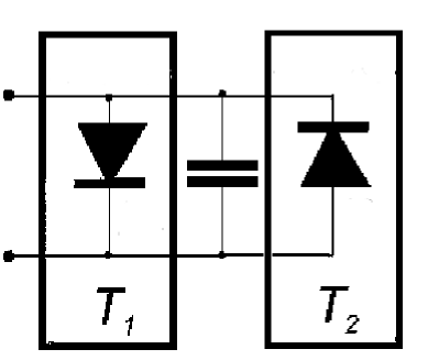
Figure 3: Brillouin’s diode engine 34 .

If $u$ is the voltage of the capacitor and $i_{1},i_{2}$ are currents through two nonlinear resistors then

$$i_{1}R_{1}(u)+u=v_{1}(t)\;\;\;\mbox{and}\;\;\;i_{2}R_{2}(u)+u=v_{2}(t),$$ (29)

where $v_{1}(t)$ and $v_{2}(t)$ are Nyquist stochastic electromotive forces 35 , due to thermal agitation in the corresponding resistors, satisfying 36

$$<v_{i}(t)>\,=0,\;\;\;<v_{i}(t)\,v_{j}(t^{\prime})>\,=2k_{B}T_{i}R_{i}\,\delta_{ij}\,\delta(t-t^{\prime}).$$ (30)

But $i_{1}+i_{2}=\dot{q}$, where $q=Cu$ is the charge of the capacitor with capacitance $C$. Therefore (29) indicate the following Langevin equation

$$\dot{u}=-\frac{u}{R(u)\,C}+\frac{v_{1}(t)}{R_{1}(u)\,C}+\frac{v_{2}(t)}{R_{2}(u)\,C},$$ (31)

where

$$R(u)=\frac{R_{1}(u)\,R_{2}(u)}{R_{1}(u)+R_{2}(u)}.$$

Using Stratonovich prescription, the drift and diffusion coefficient functions can be calculated from (31) in the manner described in the previous section for the equation (6). the results are

$$D^{(1)}(u)=\frac{u}{R(u)\,C}+\frac{k_{B}T_{1}R_{1}^{\prime}(u)}{R_{1}^{2}(u)\,C^{2}}+\frac{k_{B}T_{2}R_{2}^{\prime}(u)}{R_{2}^{2}(u)\,C^{2}},\;\;\;D^{(2)}(u)=\frac{2k_{B}}{C^{2}}\left[\frac{T_{1}}{R_{1}(u)}+\frac{T_{2}}{R_{2}(u)}\right],$$ (32)

where the prime denotes differentiation with respect to $u$.

The Fokker-Planck equation that follows

$$\frac{\partial P(u,t)}{\partial t}+\frac{\partial J(u,t)}{\partial u}=0$$

has the following probability current

$$J(u,t)=-\frac{uP(u,t)}{R(u)\,C}-\frac{k_{B}}{C^{2}}\left(\frac{T_{1}}{R_{1}(u)}+\frac{T_{2}}{R_{2}(u)}\right)\,\frac{\partial P(u,t)}{\partial u}$$ (33)

in agreement with 33 ; 34 .

The steady state operation (stationary solution of (33)) now corresponds to the vanishing probability current because evidently $J(\pm\infty,t)=0$. Then (33) produces a simple homogeneous linear differential equation for $P(u)$ with the solution

$$P(u)=P_{0}\,\exp{\left\{-\frac{C}{k_{B}}\int\limits_{0}^{u}\frac{R_{1}(u)+R_{2}(u)}{T_{1}R_{2}(u)+T_{2}R_{1}(u)}\,u\,du\right\}}.$$ (34)

If $T_{1}=T_{2}=T$, (34) reduces to the Boltzmann distribution

$$P(u)=P_{0}\,\exp{\left\{-\frac{Cu^{2}}{2k_{B}T}\right\}}$$

as should be expected for the capacitor’s energy in thermal equilibrium. The Boltzmann distribution is symmetric in $u$ and therefore $<u>\,=0$. Not surprisingly, the Second Law wins in isothermal situation irrespective of the volt-ampere characteristics of the diodes, and no self-charging of the capacitor takes place.

If temperatures are different, however, the distribution (34) is no more symmetric (note that for identical diodes $R_{2}(u)=R_{1}(-u)$). Therefore, if you feed the Brillouin demon with an external energy input, which maintains the necessary temperature difference, it will operate successfully.

Let us now consider the heat exchange between the two thermal baths 36 ; 37 . During a small time period $\Delta t$, the electromotive force $v_{1}$ performs a work $\int i_{1}v_{1}dt$ and therefore this amount of energy is taken from the first thermal bath at temperature $T_{1}$. But a part of this energy, namely $\int i_{1}^{2}R_{1}dt$, is returned back to the bath as the nonlinear resistor dissipates the Joule heat into the bath. Therefore, the net energy taken from the first bath equals

$$\Delta Q_{1}=\int\limits_{t}^{t+\Delta t}i_{1}(v_{1}-i_{1}R_{1})\,dt^{\prime}=\int\limits_{t}^{t+\Delta t}i_{1}u\,dt^{\prime}=\int\limits_{t}^{t+\Delta t}\frac{v_{1}-u}{R_{1}}\,u\,dt^{\prime}\approx-\frac{u^{2}}{R_{1}}\Delta t+\int\limits_{t}^{t+\Delta t}\frac{u}{R_{1}}\,v_{1}(t^{\prime})\,dt^{\prime}.$$

In the remaining stochastic integral, $\frac{u}{R_{1}}$ has to be replaced, according to the Stratonovich prescription, with its value at the middle of the time interval, at time $t+\frac{\Delta t}{2}$, which approximately equals

$$\frac{u}{R_{1}}+\frac{\Delta t}{2}\,\frac{d}{du}\left(\frac{u}{R_{1}}\right)\dot{u}=\frac{u}{R_{1}}+\frac{\Delta t}{2}\,\frac{d}{du}\left(\frac{u}{R_{1}}\right)\left(-\frac{u}{R\,C}+\frac{v_{1}(t)}{R_{1}\,C}+\frac{v_{2}(t)}{R_{2}\,C}\right),$$

where now $u$ is evaluated at time $t$. Therefore, taking an ensemble average, we get

$$<\Delta Q_{1}>\,=\left[-\frac{u^{2}}{R_{1}}+\frac{k_{B}T_{1}}{C}\,\frac{d}{du}\left(\frac{u}{R_{1}}\right)\,\right]\Delta t.$$

Now we average $<\Delta Q_{1}>/\Delta t$ over the voltage distribution $P(u)$ and get the heat absorbed from the first reservoir at temperature $T_{1}$ per unit time

$$\dot{Q}_{1}=\int\limits_{-\infty}^{\infty}\left[-\frac{u^{2}}{R_{1}}+\frac{k_{B}T_{1}}{C}\,\frac{d}{du}\left(\frac{u}{R_{1}}\right)\,\right]P(u)\,du=-\int\limits_{-\infty}^{\infty}\left[\frac{k_{B}T_{1}}{CR_{1}(u)}\,\frac{\partial P(u)}{\partial u}+\frac{u}{R_{1}(u)}P(u)\right]u\,du$$

in agreement with 33 ; 34 . The last step here follows from $P(\pm\infty)=0$ when integration by parts is applied.

Note that

$$\dot{Q}_{1}+\dot{Q}_{2}=-\int\limits_{-\infty}^{\infty}\left[\frac{u}{R(u)}P(u)+\frac{k_{B}}{C}\left(\frac{T_{1}}{R_{1}(u)}+\frac{T_{2}}{R_{2}(u)}\right)\frac{\partial P(u)}{\partial u}\right]u\,du=\int\limits_{-\infty}^{\infty}J(u)\,u\,du=0$$

when J=0. In other words, the heat dissipated into the second reservoir at temperature $T_{2}$ per unit time equals to the heat absorbed from the first reservoir per unit time. Therefore $\dot{Q}\equiv\dot{Q}_{1}$ is just the heat flux from the first thermal bath to the second and

$$\dot{Q}=\int\limits_{-\infty}^{\infty}\left[-\frac{u^{2}}{R_{1}(u)}+\frac{k_{B}T_{1}}{C}\,\frac{d}{du}\left(\frac{u}{R_{1}(u)}\right)\,\right]P(u)\,du$$ (35)

To have some impression of the magnitude of this flux, we approximate the volt-ampere characteristics of the diodes by a step function

$$R_{1}(u)=R_{2}(-u)=R_{+}\,\theta(u)+R_{-}\,\theta(-u)=\left\{\begin{tabular}[]{cc}$R_{+}$, if $u>0$,\\ $R_{-}$, if $u<0$.\end{tabular}\right.$$

When

$$\frac{d}{du}\left(\frac{u}{R_{1}(u)}\right)=\frac{d}{du}\left[\frac{u}{R_{+}}\theta(u)+\frac{u}{R_{-}}\theta(-u)\right]=\frac{\theta(u)}{R_{+}}+\frac{\theta(-u)}{R_{-}}+\left(\frac{1}{R_{+}}-\frac{1}{R_{-}}\right)u\,\delta(u).$$

But $u\,\delta(u)=0$ and a straightforward calculation gives the heat flux which is linear in the temperature difference 34

$$\dot{Q}=\frac{k_{B}(T_{1}-T_{2})}{C(R_{+}+R_{-})}.$$ (36)

For ideal diodes with infinite backward resistance, $\dot{Q}=0$ and there is no heat exchange between thermal reservoirs under zero load. Therefore one expects that the efficiency of the ideal diode engine tends to the Carnot efficiency $1-T_{2}/T_{1}$ when the external load tends to zero. This fact was indeed demonstrated in 34 .

V Mirror World and how it can assist demons

Mirror world was introduced in 1966 by Kobzarev, Okun, and Pomeranchuk 38 (a first-hand historical account can be found in 39 ), although the basic idea dates back to Lee and Yang’s 1956 paper 40 and subsequently was rediscovered in the modern context of renormalizable gauge theories in 42 .

The idea behind mirror matter is simple and can be explained as follows 43 . The naive parity operator P, representing the space inversion, interchanges left and right. But in case of internal symmetries, when there are several equivalent left-handed states and several equivalent right-handed states, it is not a priori obvious what right-handed state should correspond to a given left-handed state. All operators of the type SP, where S is an internal symmetry operator, are equivalent. If we can find some internal symmetry M, for which MP remains unbroken in the real world, then we can say that the world is left-right symmetric in over-all because MP is as good as the parity operator, as is P itself.

What remains is to find an appropriate internal symmetry M. Not every choice of M leads to the mirror world in a sense of a decoupled hidden sector. For example, the most economical first try is the charge conjugation operator C in the role of M 44 ; 45 ; 46 . In this case mirror world coincides with the world of antiparticles. But CP is not conserved and therefore such a world is not left-right symmetric.

Then the most natural and secure way to enforce the left-right symmetry is to double our Standard Model world by introducing a mirror twin for every elementary particle in it and arrange the right-handed mirror weak interactions, so that every P-asymmetry in ordinary world is accompanied by the opposite P-asymmetry in the hidden mirror sector. This new mirror sector must be necessarily hidden, that is only very weak interactions between mirror and ordinary particles may be allowed, otherwise this scenario will come to immediate conflict with phenomenology 38 .

If the parity symmetry in our world is indeed restored at the expense of the hidden mirror sector, many interesting phenomenological and astrophysical consequences follow that were discussed many times in the literature. It would be boring to repeat all this here. Therefore I cite only some review articles 39 ; 47 ; 48 ; 49 ; 50 where relevant references can be found. Instead of following the well-known trails, I choose a new pathway to the mirror world, with boron trifluoride ($BF_{3}$) as our rather exotic guide.

Boron trifluoride is a highly toxic, colorless, nonflammable gas with a pungent odor, used heavily in the semiconductor industry. But what is relevant for us here is the shape of its planar molecule. Three fluorine atoms seat at the corners of a equilateral triangle with the boron atom in the center. This shape is obviously parity invariant, with parity identified with the reflection in the $y$-axis of the $x-y$ plane. But the world is quantum mechanical after all and what is obvious from the classical point of view often ceases to be obvious in quantum world. So we need a quantum theory of shapes 51 ; 51a .

Let us consider rotations of the boron trifluoride molecule. The translational motion is ignored as it does not lead to anything non-trivial. Therefore it will be assumed that the center of the molecule with the boron atom at it is fixed at the origin. Then any configuration of the fluorine atoms can be obtained from a standard configuration, with one of the fluorine atoms at the positive y-axis, by some rotation

$$R(\phi)=\left(\begin{tabular}[]{cc}$\cos{\phi}$&$\sin{\phi}$\\ $-\sin{\phi}$&$\cos{\phi}$\end{tabular}\right).$$

But rotations by $\phi=\frac{2\pi}{3}\,n$, $n$-integer transform the molecule into itself because of symmetry of the equilateral triangle. Therefore the configuration space for the rotational motion of the boron trifluoride molecule is the coset space

$$Q=SO(2)/Z_{3},$$

where $Z_{3}$ is the cyclic subgroup of $SO(2)$ generated by $R(2\pi/3)$.

Topologically SO(2) is the same as the unite circle $S^{1}$ and is thus infinitely connected, because loops with different winding numbers around the circle belong to the different homotopy classes. The configuration space $Q$ is obtained from $S^{1}$ by identifying points related by rotations with $\phi=\frac{2\pi}{3}\,n$, $n$-integer. Therefore $Q$ is also infinitely connected. The multiple connectedness brings a new flavour in quantization and makes it not quite trivial 52 ; 53 . For our goals, the convenient approach is the one presented in 54 ; 55 for quantum mechanics on the circle $S^{1}$.

Naively one expects the free dynamics of any quantum planar-rotator, such as the boron trifluoride molecule, to be defined by the Hamiltonian

$$\hat{H}=\frac{\hat{L}^{2}}{2I},$$ (37)

where ($\hbar=1$)

$$\hat{L}=-i\frac{\partial}{\partial\phi}$$ (38)

is the angular momentum operator satisfying the canonical commutation relation

$$[\hat{\phi},\hat{L}]=i.$$ (39)

However, there are many pitfalls in using the commutation relation (39) in the context of the quantum-mechanical description of angle variable 56 . The locus of problems lies in the fact that $\hat{\phi}$ is not a good position operator for the configuration space $Q$, as it is multi-valued. Classically every point from $Q$ is uniquely determined by a complex number $q=\exp{(-3i\phi)}$. Therefore one can expect that the unitary operator

$$\hat{q}=\exp{(-3i\hat{\phi})},$$ (40)

is more suitable as the position operator on $Q$ 57 . From (39) we expect the commutation relations

$$[\hat{L},\hat{q}]=-3\,\hat{q},\;\;\;[\hat{L},\hat{q}^{+}]=3\,\hat{q}^{+},$$ (41)

which we assume to hold, although the self-adjoint angular momentum operator has not necessarily have to be in the naive form (38).

The representation of the algebra (41) is simple to construct 54 ; 55 . The operator $\hat{L}$, being self-adjoint, has an eigenvector $|\alpha>$ with a real eigenvalue $3\alpha$:

$$\hat{L}\,|\alpha>\,=3\alpha\,|\alpha>,\;\;\;<\alpha|\alpha>\,=1.$$

The commutation relations (41) show that $\hat{q}$ and $\hat{q}^{+}=\hat{q}^{-1}$ act as lowering and rising operators because

$$\hat{L}\,\hat{q}\,|\alpha>\,=\left([\hat{L},\hat{q}]+\hat{q}\hat{L}\right)|\alpha>\,=3(\alpha-1)\hat{q}\,|\alpha>\;\;\mbox{and}\;\;\hat{L}\,\hat{q}^{+}\,|\alpha>\,=3(\alpha+1)\hat{q}^{+}\,|\alpha>.$$

Therefore we can consider the states

$$|n+\alpha>\,=\left(\hat{q}^{+}\right)^{n}|\alpha>,\;\;n=0,\pm 1,\pm 2,\ldots$$

as spanning the Hilbert space ${\cal H}_{(\alpha)}$ where the fundamental operators $\hat{L}$ and $\hat{q}$ are realized, because, as it follows from the self-adjointness of $\hat{L}$ and unitarity of $\hat{q}$, the set of state vectors $|n+\alpha>$ forms the orthocomplete system

$$<n+\alpha|m+\alpha>\,=\delta_{nm},\;\;\sum\limits_{n=-\infty}^{\infty}|n+\alpha><n+\alpha|=1.$$

The angular momentum operator is diagonal in this basis $\hat{L}\,|n+\alpha>\,=3(n+\alpha)\,|n+\alpha>$, and so does the Hamiltonian (37). The energy eigenvalues are

$$E_{n}=\frac{9(n+\alpha)^{2}}{2I}.$$ (42)

For each $\alpha$, there is a vacuum state corresponding to $n=0$ and these vacuum states are in general different, like $\theta$-vacuums in QCD. More precisely, ${\cal H}_{(\alpha)}$ and ${\cal H}_{(\beta)}$ are unitary equivalent representation spaces of the algebra (41) if and only if the difference between $\alpha$ and $\beta$ is an integer 54 ; 55 . Therefore, in contrast to the canonical commutation relations, the algebra (41) has infinitely many inequivalent unitary representations parameterized by a continuous parameter $\alpha$ from the interval $0\leq\alpha<1$.

The spectrum (42) is doubly degenerate for $\alpha=0$, because in this case $E_{n}=E_{-n}$, as well as for $\alpha=1/2$, because then $E_{n}=E_{-(n+1)}$. For other values of $\alpha$, there is no degeneracy. This degeneracy reflects invariance under the parity transformation 55 .

As we had already mentioned, geometrically the parity transformation is the reflection in the $y$-axis, that is inversion of $S^{1}$ around a diameter. Classically the parity transformation moves the point specified by the angle $\phi$ to the one specified by the angle $-\phi$, if we measure an angular coordinate $\phi$ from the axis fixed under the parity operation. Therefore it is natural for the quantum mechanical unitary parity operator $\hat{P}$ on $Q$ to satisfy

$$\hat{P}^{+}\,\hat{q}\,\hat{P}=\hat{q}^{+},\;\;\hat{P}^{+}\,\hat{L}\,\hat{P}=-\hat{L}.$$ (43)

Such a parity operator is an automorphism of the fundamental algebra (41), but can not always be realized in the Hilbert space ${\cal H}_{(\alpha)}$. Indeed,

$$\hat{L}\,\hat{P}\,|n+\alpha>\,=-\hat{P}\,\hat{L}\,|n+\alpha>\,=-3(n+\alpha)\hat{P}\,|n+\alpha>$$

shows that $\hat{P}\,|n+\alpha>$ does not in general lies in ${\cal H}_{(\alpha)}$, unless $\alpha=0$ or $\alpha=1/2$. Otherwise $\hat{P}\,|n+\alpha>\,\in{\cal H}_{(1-\alpha)}$. Therefore only for $\alpha=0$ or $\alpha=1/2$ is parity a good symmetry and other realizations of quantum mechanics on $Q$ break parity invariance. In later cases, to restore parity invariance requires doubling of the Hilbert space by considering ${\cal H}_{(\alpha)}\oplus{\cal H}_{(1-\alpha)}$.

It is rather strange that most realizations of the quantum shape of the boron trifluoride molecule violate parity, although classically the molecule is reflection symmetric. After all no microscopic source of parity violation was assumed in the molecular dynamics. How then does parity violation emerge in the shape? This happens because we concentrated on the slow nuclear degrees of freedom and completely neglected the fast electronic motion. A general argument is given in 51 ; 51a that in a complete theory, with fast degrees of freedom included, there is no parity violation. For example, in molecular physics the coupling between rotational modes and the electronic wave functions lead to transitions between these wave functions related by parity, with time scales much longer than typical rotational time scales. As a result, parity invariance is restored but nearly degenerate states of opposite parity, the parity doubles, appear in the molecular spectra.

To get an intuitive understanding why different quantum theories are possible on $Q$ and why most of them violate parity, it is instructive to find the explicit form for the angular momentum operator in each $\alpha$-realization 54 ; 55 .

Let

$$|\theta>\,=\sum\limits_{n=-\infty}^{\infty}a_{n}\,|n+\alpha>$$

be an eigenvector of the position operator $\hat{q}^{+}$:

$$\hat{q}^{+}\,|\theta>\,=e^{\,3i\theta}\,|\theta>.$$

Then we get the recurrent relation

$$a_{n}=e^{-3i\theta}\,a_{n-1}$$

and, therefore, up to normalization

$$|\theta>\,=e^{i\,\omega(\theta)}\sum\limits_{n=-\infty}^{\infty}e^{-3in\theta}\,|n+\alpha>,$$

where $\omega(\theta)=\omega(\theta+2\pi/3)$ is an arbitrary phase. But then

$$e^{-i\lambda\hat{L}}\,|\theta>\,=e^{-3i\lambda\alpha}\,e^{i\,\omega(\theta)}\,e^{-i\omega(\theta+\lambda)}\,|\theta+\lambda>.$$

Let $|\psi>$ be an arbitrary state vector. Differentiating the equality

$$<\theta|e^{i\lambda\hat{L}}|\psi>=\left(<\psi|e^{-i\lambda\hat{L}}|\theta>\right)^{+}=e^{3i\lambda\alpha}\,e^{-i\omega(\theta)}\,e^{i\,\omega(\theta+\lambda)}<\theta+\lambda|\psi>$$

with respect to $\lambda$ and taking $\lambda=0$ in the result multiplied by $-i$, we get

$$<\theta|\hat{L}|\psi>=\left[-i\frac{\partial}{\partial\theta}+3\alpha+\frac{\partial\omega}{\partial\theta}\right]\psi(\theta),$$

where $\psi(\theta)=<\theta|\psi>$ is the wave function. Therefore, in the $q$-representation, where $\hat{q}$ is diagonal, the angular momentum operator is

$$\hat{L}=-i\frac{\partial}{\partial\theta}+A(\theta),$$ (44)

with

$$A(\theta)=3\alpha+\frac{\partial\omega(\theta)}{\partial\theta}$$ (45)

playing the role of a gauge field.

As we see, the $\alpha$-quantum theory on $Q$ is analogous to the quantum theory on a unit circle with the vector potential (45) along the circle. Then we have the magnetic flux

$$\int\vec{B}\cdot d\vec{S}=\oint\vec{A}\cdot d\vec{l}=6\pi\alpha$$

piercing the circle perpendicularly to the $x-y$ plane. Classically a charged particle on the circle does not feel the magnetic flux, if the the magnetic field on the circle is zero, but quantum mechanically it does – the Aharonov-Bohm effect. Therefore it is not surprising that we have many different quantum theories, nor is it surprising that parity is violated 58 . It is also clear that in a more complete theory, including sources of the magnetic flux, parity is not violated 58 .

Now back to demons. Suppose parity invariance is indeed restored in a manner advocated by mirror matter proponents. Then some non-gravitational interactions are not excluded between the ordinary and mirror sectors. One interesting possibility is the photon-mirror photon kinetic mixing interaction

$${\cal{L}}=\frac{\epsilon}{2}F^{\mu\nu}F^{\,\prime}_{\mu\nu},$$

where $F^{\mu\nu}$ and $F^{\,\prime}_{\mu\nu}$ are the field strength tensors for electromagnetism and mirror electromagnetism respectively. As a result ordinary and mirror charged particles interact electromagnetically with the interaction strength controlled by the mixing parameter $\epsilon$. A number of observed anomalies can be explained from mirror matter perspective if

$$\epsilon\sim 5\cdot 10^{-9}$$ (46)

(see 47 and references wherein).

Remarkably, this tiny electromagnetic interaction is nevertheless sufficient for thermal equilibration to occur in a mixture of ordinary and mirror matter at Earth-like temperatures 59 , and to provide a force strong enough to oppose the force of gravity, so that a mirror matter fragment can remain on the Earth’s surface instead of falling toward its center 59a . Demons considered above can clearly benefit from this fact. What is necessary is to add a significant amount of mirror matter to the thermal reservoir we want to operate at colder temperature. Mirror matter will draw in heat from the surrounding ordinary component of the thermal bath and radiate it away as mirror photons. Thereby an effective cooling will take place and the necessary temperature difference will be created between the thermal baths (assuming the another bath do not contain a mirror component), even if initially the temperatures were the same.

Equation (36) indicates that, at least for some demons, heat exchange between two thermal reservoirs of the demon can be made very low. Consequently, mirror matter walls of the colder reservoir should radiate a very small flux of mirror electromagnetic energy at dynamical equilibrium and hence must be very cold. In fact, it appears that for significant amount of mirror matter the corresponding reservoir would be cooled to near absolute zero where approximations of reference 59 break down. Therefore we refrain from any detailed calculations.

VI Conclusion

As frequently stressed by Landau 39 , we expect the world of elementary particles to be mirror symmetric because the space itself is mirror symmetric. But weak interactions turned out to be left-handed and heroic efforts of Landau and others 44 ; 45 ; 46 to save left-right symmetry by CP also failed. Therefore we are left with the strange fact that nature is left-right asymmetric. But the example from the molecular physics considered above suggests a possibility that the observed asymmetry might be just apparent, the result of the fact that some fast degrees of freedom hidden, presumably, at the Planck scale, were overlooked. Then in the more complete theory parity symmetry will be restored, but the parity doubles will appear at the universe level in the form of mirror world 38 ; 42 .

If nature is indeed organized in this manner, the fascinating Maxwell demons considered in the previous sections can be made operative by just adding mirror matter to one of their thermal reservoirs. Mirror matter demons can extract heat from one thermal reservoir, for example from the world ocean, and transform it very effectively (in case of Brillouin demon) to some useful work, thereby solving the global energy problems of mankind!

All this “sounds too good to be true” 60 . But the principal question is whether mirror matter exists. If it does indeed exist and if the photon-mirror photon mixing is not negligibly small I do not see how the mirror demons can fail.

As for the photon-mirror photon mixing, the proposition that its magnitude is of the order of (46) is experimentally falsifiable in near future, because such mixing leads to orthopositronium to mirror orthopositronium oscillations and as a result to invisible decays of orthopositronium in vacuum, with intensities accessible in the experiment 61 which is under way.

Maybe the putative perspective of using mirror matter demons will appear a little less exotic if we recall that, in a sense, we are all made of demons. I mean that the Brownian ratchet engines, which operate extremely effectively and reliably, can be found in every biological cell 62 ; 63 ; 64 . Therefore I would be not much surprised if someday nanotechnology will find the mirror matter useful, provided, of course, that it exists at all.

The idea that mirror matter can find applications in heat engines I credit to Saibal Mitra 60 . But not his notes served as an inspiration for this investigation. The paper emerged from J. D. Norton’s advise to be a little more critical about Landauer’s exorcism of Maxwell’s demon in response to my rather careless claim in 65 that Landauer’s principle killed the demon. “O King, most high and wise Lord; How incomprehensible are thy judgments, and inscrutable thy ways!”

References

- (1) A. S. Eddington, The Nature of the Physical World (Macmillan, New York, 1929), p. 74.
- (2) J. D. Collier, Two Faces of Maxwell’s Demon Reveal the Nature of Irreversibility; Studies in the History and Philosophy of Science 21, 257 (1990).
- (3) J. Earman and J. D. Norton, Exorcist XIV: The Wrath of Maxwell’s Demon. Part I. From Maxwell to Szilard; Studies in the History and Philosophy of Modern Physics 29, 435 (1998).
- (4) H. S. Lef and A. F. Rex (Eds.), Maxwell’s Demon 2: Entropy, Classical and Quantum Information, Computing (Institute of Physics Publishing, Bristol and Philadelphia, 2003).
- (5) R. Landauer, Irreversibility and heat generation in the computing process; IBM Journal of Research and Development 5, 183 (1961).
- (6) M. B. Plenio and V. Vitelli, The physics of forgetting: Landauer’s erasure principle and information theory; Contemporary Physics 42, 25 (2001).
- (7) C. H. Bennett, Notes on Landauer’s principle, reversible computation, and Maxwell’s Demon; Studies in the History and Philosophy of Modern Physics 34, 501 (2003).
- (8) J. Earman and J. D. Norton, Exorcist XIV: The Wrath of Maxwell’s Demon. Part II. From Szilard to Landauer and Beyond; Studies in the History and Philosophy of Modern Physics 30, 1 (1999).
- (9) J. D. Norton, Eaters of the Lotus: Landauer’s Principle and the Return of Maxwell’s Demon; Studies in the History and Philosophy of Science 36, 375 (2005).
- (10) A. E. Allahverdyan and Th. M. Nieuwenhuizen, Unmasking Maxwell’s Demon; AIP Conference Proceedings 643, 436 (2002).
- (11) Kechen Zhang and Kezhao Zhang, Mechanical models of Maxwell’s demon with noninvariant phase volume; Phys. Rev. A 46, 4598 (1992).
- (12) K. Shizume, Heat generation required by information erasure; Phys. Rev. E 52, 3495 (1995).
- (13) B. Piechocinska, Information Erasure; Phys. Rev. A 61, 062314 (2000).
- (14) A. E. Allahverdyan and Th. M. Nieuwenhuizen, Breakdown of the Landauer bound for information erasure in the quantum regime; Phys. Rev. E 64, 056117 (2001).
-
(15)
S. Goldstein, Boltzmann’s Approach to Statistical Mechanics;
http://arxiv.org/abs/cond-mat/0105242 - (16) R. Penrose, The Emperor’s New Mind (Oxford University Press, Oxford, 1989), p. 343.
- (17) H. Price, On the origins of the arrow of time: why there is still a puzzle about the low entropy past; In Christopher Hitchcock, ed., Contemporary Debates in the Philosophy of Science (Blackwell, Oxford, 2004), pp. 219-239.
- (18) J. Eggers, Sand as Maxwell’s Demon; Phys. Rev. Lett. 83, 5322 (1999).
- (19) P. A. Skordos and W. H. Zurek, Maxwell’s demon, rectifiers, and the second law: Computer simulation of Smoluchowski’s trapdoor; Am. J. Phys. 60, 876 (1992).
- (20) A. Rex and R. Larsen, Entropy And Information For An Automated Maxwell’s Demon; In Harvey S. Leff and Andrew Rex, eds., Maxwell’s Demon 2: Entropy, Classical and Quantum Information, Computing (Institute of Physics Publishing, Bristol and Philadelphia, 2003), pp. 101-109.
- (21) R. P. Feynman, R. B. Leighton and M. Sands, The Feynman Lectures on Physics (Addison-Wesley, Reading, MA, 1963), Vol. 1, pp. 46.1-46.9; The idea goes back to Smoluchowski: M. von Smoluchowski, Experimentell nachweisbare der ublichen Thermodynamik widersprechende Molekularphanomene; Phys. Z. 13, 1069 (1912).
- (22) J. M. R. Parrondo and P. Español, Criticism of Feynman’s analysis of the ratchet as an engine; Am. J. Phys. 64, 1125 (1996).
- (23) M. O. Magnasco and G. Stolovitzky, Feynman’s Ratchet and Pawl; J. Statist. Phys. 93, 615 (1998).
- (24) T. Munakata and D. Suzuki, Rectification Efficiency of the Feynman Ratchet; J. Phys. Soc. Jap. 74, 550 (2005).
- (25) A. Gomez-Marin and J. M. Sancho, Ratchet, pawl and spring Brownian motor; PhysicaD 216, 214 (2006).
- (26) H. Risken, The Fokker-Planck Equation (Springer, Berlin, 1984).
- (27) N. G. van Kampen, Itô versus Stratonovich; J. Statist. Phys. 24, 175 (1981).
- (28) C. W. Gardiner, Adiabatic elimination in stochastic systems. I. Formulation of methods and application to few-variable systems; Phys. Rev. A 29, 2814 (1984).
- (29) A. E. Siegman, Simplified derivation of the Fokker-Planck equation; Am. J. Phys. 47, 545 (1979).
- (30) E. Kamke, Handbook on Ordinary Differential Equations; (Nauka, Moscow, 1976), p. 35 (in Russian).
- (31) L. Brillouin, Can the Rectifier Become a Thermodynamical Demon? Phys. Rev. 78, 627 (1950).
- (32) R. McFee, Self-Rectification in Diodes and the Second Law of Thermodynamics; Am. J. Phys. 39, 814 (1971).
- (33) I. M. Sokolov, On the energetics of a nonlinear system rectifying thermal fluctuations; Europhys. Lett. 44, 278 (1998).
- (34) I. M. Sokolov, Reversible fluctuation rectifier; Phys. Rev. E 60, 4946 (1999).
- (35) H. Nyquist, Thermal Agitation of Electric Charge in Conductors; Phys. Rev. 32, 110 (1928).
- (36) R. van Zon, S. Ciliberto, E. G. D. Cohen, Power and heat fluctuation theorems for electric circuits; Phys. Rev. Lett. bf 92, 130601 (2004).
- (37) K. Sekimoto, Energetics Of Thermal Ratchet Models; http://arxiv.org/abs/cond-mat/9611005
- (38) I. Yu. Kobzarev, L. B. Okun and I. Ya. Pomeranchuk, On the possibility of observing mirror particles; Sov. J. Nucl. Phys. 3, 837 (1966).
- (39) L. B. Okun, Mirror particles and mirror matter: 50 years of speculations and searches; http://arxiv.org/abs/hep-ph/0606202
- (40) T. D. Lee and C. N. Yang, Question Of Parity Conservation In Weak Interactions; Phys. Rev. 104, 254 (1956).
- (41) R. Foot, H. Lew and R. R. Volkas, A Model with fundamental improper space-time symmetries; Phys. Lett. B 272, 67 (1991).
- (42) Z. K. Silagadze, Mirror Objects In The Solar System? Acta Phys. Polon. B 33, 1325 (2002).
- (43) L. D. Landau, On The Conservation Laws For Weak Interactions; Nucl. Phys. 3, 127 (1957).
- (44) G. C. Wick, A. S. Wightman and E. P. Wigner, The intrinsic parity of elementary particles; Phys. Rev. 88, 101 (1952).
- (45) E. P. Wigner, Relativistic Invariance And Quantum Phenomena; Rev. Mod. Phys. 29, 255 (1957).
- (46) R. Foot, Mirror matter-type dark matter; Int. J. Mod. Phys. D 13, 2161 (2004); Experimental implications of mirror matter-type dark matter; Int. J. Mod. Phys. A 19, 3807 (2004).
- (47) Z. Berezhiani, Mirror world and its cosmological consequences; Int. J. Mod. Phys. A 19, 3775 (2004).
- (48) P. Ciarcelluti, Cosmology of the mirror universe; http://arxiv.org/abs/astro-ph/0312607
- (49) Z. K. Silagadze, TeV scale gravity, mirror universe, and … dinosaurs; Acta Phys. Polon. B 32, 99 (2001).
- (50) A. P. Balachandran, A. Simoni and D. M. Witt, Molecules As Quantum Shapes And How They Violate P And T; Int. J. Mod. Phys. A 7, 2087 (1992).
- (51) A. P. Balachandran and S. Vaidya, Emergent chiral symmetry: Parity and time reversal doubles; Int. J. Mod. Phys. A 12, 5325 (1997).
- (52) L. Schulman, A Path integral for spin; Phys. Rev. 176, 1558 (1968).
- (53) A. P. Balachandran, Classical Topology And Quantum Statistics; Int. J. Mod. Phys. B 5, 2585 (1991).
- (54) Y. Ohnuki and S. Kitakado, Fundamental algebra for quantum mechanics on and gauge potentials; J. Math. Phys. 34, 2827 (1993).
- (55) S. Tanimura, Gauge field, parity and uncertainty relation of quantum mechanics on ; Prog. Theor. Phys. 90, 271 (1993).
- (56) P. Carruthers and M. M. Nieto, Phase and angle variables in quantum mechanics; Rev. Mod. Phys. 40, 411 (1968).
- (57) J. M. Levy-Leblond, Who Is Afraid Of Nonhermitian Operators? A Quantum Description Of Angle And Phase; Annals Phys. 101, 319 (1976).
- (58) S. Olariu and I. I. Popescu, The quantum effects of electromagnetic fluxes; Rev. Mod. Phys. 57, 339 (1985).
- (59) R. Foot and S. Mitra, Detecting mirror matter on earth via its thermal imprint on ordinary matter; Phys. Lett. A 315, 178 (2003).
- (60) S. Mitra and R. Foot, Detecting dark matter using centrifuging techniques; Phys. Lett. B 558, 9 (2003).
- (61) S. Mitra, Applications of mirror matter; http://people.zeelandnet.nl/smitra/applications.htm
- (62) A. Badertscher et al., An apparatus to search for mirror dark matter via the invisible decay of orthopositronium in vacuum; Int. J. Mod. Phys. A 19, 3833 (2004).
- (63) M. Bier, Brownian ratchets in physics and biology; Contemp. Phys. 38, 371 (1997).
- (64) R. D. Astumian, Thermodynamics and kinetics of a Brownian motor; Science 276, 917 (1997).
- (65) G. Oster and H. Wang, Rotary protein motors; Trends in Cell Biology 13, 114 (2003).
- (66) Z. K. Silagadze, Zeno meets modern science; Acta Phys. Polon. B 36, 2887 (2005).