Performance of the CDF Calorimeter Simulation in Tevatron Run II

Abstract

The CDF experiment is successfully collecting data from $\mathrm{p}\bar{\mathrm{p}}$ collisions at the Tevatron in Run II. As the data samples are getting larger, systematic uncertainties due to the measurement of the jet energy scale assessed using the calorimeter simulation have become increasingly important. In many years of operation, the collaboration has gained experience with GFLASH, a fast parametrization of electromagnetic and hadronic showers used for the calorimeter simulation. We present the performance of the calorimeter simulation and report on recent improvements based on a refined in situ tuning technique. The central calorimeter response is reproduced with a precision of 1-2%.

1 Introduction

Since the start of Run II in 2001, the Collider Detector at Fermilab (CDF) CDF-tdr has collected over 1 fb^-1 of data of $\mathrm{p}\bar{\mathrm{p}}$ collisions at 1.96 TeV center-of-mass energy. In a variety of resulting publications, the simulation of the calorimeter has proved to be a crucial element for the precision measurement of physical observables, like the mass of the top quark, since it appears as one of the keys to control the jet energy scale systematics. The CDF calorimeter simulation is based on GFLASH grindhammer:1990 , a FORTRAN package used for the fast simulation of electromagnetic and hadronic showers. It is embedded in a GEANT3 framework brun:1993 as part of the whole detector simulation and has various advantages w.r.t. the detailed GEANT shower simulation: In CDF it is up to 100 times faster, and it can be flexibly tuned. The calorimeter simulation was initially tuned to test beam data and has been improved due to a steadily refined in situ tuning using samples of isolated charged particles, which recently became available over a remarkably extended momentum range up to 40 GeV. Here we report on the GFLASH performance effective for current CDF physics publications and on ongoing improvements contributing to the ambitious Run II physics program.

2 CDF Calorimetry

CDF is a general-purpose charged and neutral particle detector with a calorimeter and a tracking system. The calorimeter has a central and a forward section subdivided into a total of five compartments (Fig. 1): the central electromagnetic, CEM CDF-cem , the central hadronic, CHA CDF-had , the plug electromagnetic, PEM CDF-plug , the plug hadronic, PHA CDF-plug , and the wall hadronic, WHA CDF-had . The calorimeter is of sampling type, with lead (iron) absorbers for the electromagnetic (hadronic) compartments, scintillating tiles and wavelength shifters. It is subdivided into 44 projective tower groups, each group made of 24 wedges (partially 48 in the plug part) circularly arranged around the Tevatron beam and pointing to the nominal event vertex. The central and plug part together cover the pseudorapidity range $|\eta|<3.6$. The calorimeter encloses a tracking system consisting of a vertex detector and a cylindrical drift chamber, both situated within a 1.4 T solenoid magnet. It provides a precise measurement of single charged particle momenta serving as an energy reference for the calorimeter simulation tuning.

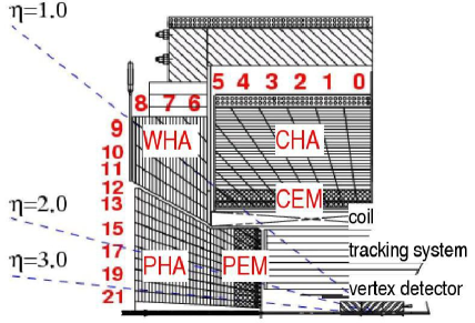
Figure 1: Left: Quadrant view of the CDF calorimeter showing the electromagnetic (CEM, PEM) and hadronic compartments (CHA, WHA, PHA). Right: Sampling structure and energy resolutions for the central (CEM, CHA) and the plug part (PEM, PHA).

3 GFLASH in a Nutshell

The CDF simulation uses GEANT to propagate particles from the main interaction point through the detector volume. A shower in GFLASH is initiated when a particle undergoes the first inelastic interaction in the calorimeter. GFLASH treats the calorimeter as one effective medium using GEANT geometry and material information. GFLASH is ideal for calorimeter modules which may have a complicated but repetitive sampling structure.

Given an incident particle energy, $E_{\mathrm{inc}}$, the visible energy in the active medium,

$$\vspace*{-4pt}\mathrm{d}E_{\mathrm{vis}}(\mathbf{r})=E_{\mathrm{inc}}\hat{m}\left[\frac{\hat{e}}{\hat{m}}c_{\mathrm{em}}f_{\mathrm{em}}(\mathbf{r})+\frac{\hat{h}}{\hat{m}}c_{\mathrm{had}}f_{\mathrm{had}}(\mathbf{r})\right]\mathrm{d}\mathbf{r}\;,\vspace*{-1pt}$$ (1)

is calculated according to the sampling fractions for electrons ($\hat{e}$) and hadrons ($\hat{h}$) relative to the sampling fraction for minimum ionizing particles ($\hat{m}$), taking their relative fractions $c_{\mathrm{em}}$ and $c_{\mathrm{had}}$ of energy deposited in the active medium into account. $f_{\mathrm{em}}(\mathbf{r})$ and $f_{\mathrm{had}}(\mathbf{r})$ are electromagnetic and hadronic spatial energy distributions of the form $f(\mathbf{r})=\frac{1}{2\pi}\,L(z)\cdot T(r,\,z)$, factorizing into a longitudinal profile $L(z)$, which is a function of the shower depth $z$, and a lateral profile $T(r,\,z)$, which depends on $z$ and on the radial distance $r$ from the shower center. The showers are treated as azimuthally symmetric.

The longitudinal electromagnetic profiles are assumed to follow a Gamma distribution,

$$L_{\mathrm{em}}(x)=\frac{x^{\alpha-1}e^{-x}}{\Gamma(\alpha)}\;,$$ (2)

where $x=\beta z$ and $z$ measured in units of radiation lengths $X_{0}$. $\alpha$ and $\beta$ are correlated parameters generated using two Gaussians, whose means and widths are free parameters subject to tuning, and a correlation matrix hardwired in GFLASH. Longitudinal hadronic shower profiles are a superposition of three shower classes:

$$L_{\mathrm{had}}(x) = f_{\mathrm{dep}}\left[c_{\mathrm{h}}\mathcal{L}_{\mathrm{h}}(x_{\mathrm{h}})+c_{\mathrm{f}}\mathcal{L}_{\mathrm{f}}(x_{\mathrm{f}})+c_{\mathrm{l}}\mathcal{L}_{\mathrm{l}}(x_{\mathrm{l}})\right]\;,$$ (3)

$$\mathcal{L}_{i}(x_{i}) = \frac{x_{i}^{\alpha_{i}-1}e^{-x_{i}}}{\Gamma(\alpha_{i})}\;\;,\;x_{i}=\beta_{i}z_{i}\;\;\;\;\;\;\;\;\;\;(i=\mathrm{h}\,,\mathrm{f}\,,\mathrm{l})\;.$$ (4)

$\mathcal{L}_{\mathrm{h}}$ is a purely hadronic component ($z_{\mathrm{h}}$ given in units of absorption lengths $\lambda_{0}$). $\mathcal{L}_{\mathrm{f}}$ accounts for the component induced by neutral pions from a first inelastic interaction ($[z_{\mathrm{f}}]=X_{0}$), and $\mathcal{L}_{\mathrm{l}}$ originates from neutral pions occurring in later stages of the shower development ($[z_{\mathrm{l}}]=\lambda_{0}$). Each subprofile in Eq. (4) is characterized by an individual correlated pair ($\alpha$, $\beta$) analogously to Eq. (2). The coefficients $c_{i}$ are the relative probabilities of the three classes expressed in terms of the fraction of showers containing a neutral pion ($f_{\pi^{0}}$) and the fraction of showers with a neutral pion in later interactions ($f^{\mathrm{l}}_{\pi^{0}}$):

$$c_{\mathrm{h}}=1-f_{\pi^{0}}\;,\;\;c_{\mathrm{f}}=f_{\pi^{0}}(1-f^{\mathrm{l}}_{{\pi^{0}}})\;,\;\;c_{\mathrm{l}}=f_{\pi^{0}}f^{\mathrm{l}}_{{\pi^{0}}}\;.$$ (5)

The global factor $f_{\mathrm{dep}}$ is the fraction of deposited energy w.r.t. the energy of the incident particle. When a shower is generated, correlations between all parameters are properly taken into account. In total, the longitudinal shower profile is described by 18 independent parameters for the hadronic part (the means and widths of the $\alpha$’s, $\beta$’s, and of the fractions $f_{\mathrm{dep}}$, $f_{\pi^{0}}$ and $f^{\mathrm{l}}_{{\pi^{0}}}$), and four parameters for the purely electromagnetic part.

The lateral energy profile at a given shower depth $z$ has the functional form

$$T(r)=\frac{2rR_{0}^{2}}{(r^{2}+R_{0}^{2})^{2}}\;.$$ (6)

The free quantity $R_{0}$ is given in units of Molière radius (for electromagnetic) or absorption lengths (for hadronic showers), respectively. $R_{0}$ is an approximate log-normal distribution with a mean and a variance parametrized as a function of the incident particle energy $E_{\mathrm{inc}}$ and shower depth $z$. The mean is given by

$$\langle R_{0}(E_{\mathrm{inc}},z)\rangle = \left[R_{1}+(R_{2}-R_{3}\ln E_{\mathrm{inc}})z\right]^{n}\;,$$ (7)

where $n$=1(2) for the hadronic (electromagnetic) case. The spread of hadronic showers increases linearly with shower depth $z$ and decreases logarithmically with $E_{\mathrm{inc}}$. Both shower types have their own set of adjustable parameter values (the $R_{i}$ plus three independent parameters for the variance), thus giving a total of 12 parameters.

After generating the profiles, GFLASH distributes the incident particle energy in discrete interval steps following the longitudinal profile, and then deposits energy spots in the simulated calorimeter volume according to the lateral profile. The number of energy spots is smeared to account for sampling fluctuations. The visible energy is obtained by integrating over the energy spots and applying the relative sampling fractions Eq. (1).

4 Gflash Tuning Method

The tuning of GFLASH mostly relies on test beams of electrons and charged pions with energies between 8 and 230 GeV currat:2002 , and has been refined during Run II using the calorimeter response of single isolated tracks in the momentum range 0.5-40 GeV/c measured in situ. The tuning of hadronic showers follows a four-step procedure.

Adjusting the MIP peak

Reproducing the response of minimum ionizing particles (MIP) is the first step since it serves as a reference for all other responses, see Eq. (1). The position and width of the simulated MIP peak is tuned to 57 GeV test beam pions in the electromagnetic compartments and involves the adjustment of charge collection efficiencies, which is handled by GEANT at this stage of the simulation.

Setting the hadronic energy scale and shape

Next, the shape of the individual energy distributions in the electromagnetic and hadronic compartment, the sum of both, and the hadronic response of MIP-like particles in the hadronic compartment are adjusted. The tuning is based on 57 GeV test beam pions and involves the most sensitive longitudinal parameters, the means and widths of $\alpha_{\mathrm{l}}$ and $\beta_{\mathrm{l}}$ (steering the shower component induced by $\pi^{0}$’s from later interactions), of $\beta_{\mathrm{h}}$ (which is related to the purely hadronic component), see Eq. (4), and of the fractions $f_{\mathrm{dep}}$ and $f_{\mathrm{{\pi^{0}}}}$ in Eqn. (3) and (5).

Fixing the energy dependence

After the longitudinal profile has been adjusted at one energy point, the other test beam samples are employed to parametrize the energy dependence of the parameters, which is typically logarithmic. At this point, also the inclusion of in situ tracks is important in order to provide a robust extrapolation into the important low energy region where test beam data are not available. A functional form $f(E_{\mathrm{inc}})=a+b\tanh(c\ln E_{\mathrm{inc}}+d)$ is used to describe the dependence of the fractions in Eqn. (3) and (5) on the incident particle energy $E_{\mathrm{inc}}$. Distinct parametrizations in the central and plug calorimeter were introduced to account for their different sampling structure. Initial Run II tunes involved samples of single isolated tracks up to 5 GeV/c in the central and plug part. Recently, the energy evolution of $f_{\mathrm{dep}}$ and the relative sampling fractions, $\hat{e}/\hat{m}$ and $\hat{h}/\hat{m}$, have been tuned using the total and MIP-like responses of in situ tracks up to 40 GeV/c (Sec. 6).

Tuning the lateral profile

The lateral profile is treated almost independently from longitudinal profile details and is tuned solely with Run II data. The parameters $R_{i}$ of Eq. (7), which have been initially adjusted to describe the profiles in the energy range 0.5-5.0 GeV/c (using default values provided by the H1 collaboration at higher energies), are now tuned up to particle momenta of 40 GeV/c (Sec. 6).

5 Impact on CDF Jet Energy Scale

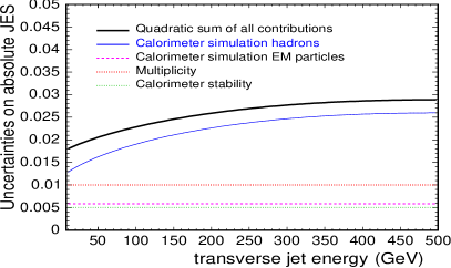
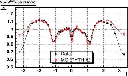
Figure 2: Left: Jet energy scale uncertainties due to calorimeter simulation and calibration published in cdfnim . Right: Di-jet balance $\beta$ vs. $\eta$ in data and simulation for transverse jet momenta 25-55 GeV/c.

We first report on the performance of the early Run II tuning embodied by CDF physics publications to date. Despite the good agreement with test beam data currat:2002 , the quality of the simulation used to be hard to control in the intermediate energy region, which is of particular importance since it constitutes a relevant fraction of the particle spectrum of a typical jet in CDF. For the initial tuning of the energy evolution of GFLASH parameters, minimum bias data providing tracks only up to 5 GeV were involved. Later checks based on special single track samples at higher momenta revealed a underestimation of the data. The level of agreement in the central was 2% for $<$12 GeV, 3% for 12 to 20 GeV, and 4% for $>$20 GeV cdfnim . Through convolution with a jet’s typical particle spectrum, these numbers directly translate into the systematic uncertainties of the jet energy scale used by CDF to date (Fig. 2, left). The dominant contribution to the total uncertainties originate from discrepancies between the simulated and measured calorimeter response and from the low statistical precision of early Run II control samples.

The inhomogeneity of the calorimeter response is accounted for by an $\eta$ dependent tuning. Jet responses in the plug and wall part are re-calibrated w.r.t. the better understood central part using a correction derived from di-jet events, $\beta=p_{\mathrm{T}}^{\mathrm{probe}}/p_{\mathrm{T}}^{\mathrm{trigger}}$, which relates the transverse momentum $p_{\mathrm{T}}$ of the non-central “probe” jet to the $p_{\mathrm{T}}$ of the central “trigger” jet. A comparison of the simulated and measured di-jet balance (Fig. 2, right) shows that the tuning is reproducing many calorimeter particularities along $\eta$.

6 In Situ Tuning Progress

The situation in the central calorimeter has now substantially improved due to the development of dedicated single track triggers with high momentum thresholds up to 15 GeV/c. The samples collected so far (a total of over 20 M events) allow a precise monitoring of the simulation performance in the energy range 0.5-40 GeV. In addition, steadily increased single track samples selected in minimum bias events now allow a consistent tuning of the plug simulation up to incident particle energies of 20 GeV.

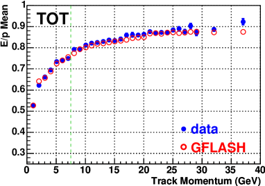
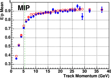
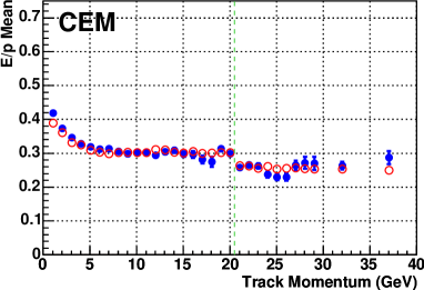
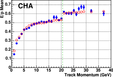
Figure 3: Simulated and measured $\langle E/p\rangle$ responses vs. track momentum in the central calorimeters CEM and CHA, the sum of both (TOT), and the CHA response of MIP-like particles (MIP). The vertical dashed lines indicate biases due to momentum dependent track analysis cuts and calculation methods.

Measurement technique

The in situ approach employs high quality tracks which are well contained within the target calorimeter tower (given by the track’s extrapolation into the electromagnetic compartment) and which are isolated within a 7$\times$7 tower block around the target tower. The signal is defined as the energy deposition seen in a 2$\times$2 block (for PEM and CEM) or a 3$\times$3 block (for CHA and PHA), respectively. For the background estimate, tower strips with the same $\eta$ range but along the edges of a 5$\times$5 tower group around the target tower are used. The simulation is usually based on a particle gun using a controlled momentum spectrum of a mixture of pions, kaons and protons, plus a minimum bias generator on top for realistic background modeling.

Absolute $\langle E/p\rangle$ response

Fig. 3 shows the comparison of the average $E/p$ responses between data and simulation based on the most recent tuning of the energy dependence of $f_{\mathrm{dep}}$, $\hat{e}/\hat{m}$ and $\hat{h}/\hat{m}$. The basic idea is to adjust simultaneously the simulated total response (TOT) and the CHA response of MIP-like particles with CEM$<670$ MeV using in situ tracks up to 40 GeV, keeping the test beam tuning at higher energies. Indeed, the simulated TOT and MIP (top) as well as the CEM and CHA responses (bottom) agree quite well with the data. The total $\langle E/p\rangle$ in the central part, which serves as an important benchmark for the systematic jet energy scale uncertainties, is reproduced with 1-2% precision within 0.5-40 GeV. The new tuning reflects more properly the current condition of the CDF calorimeter, which includes aging effects of the photomultipliers, and partially replaces the former conservative test beam uncertainties of 4 %.

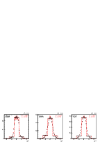
Figure 4: Top: $\chi^{2}$ contours versus GFLASH parameters $R_{1}$ and $Q$ (see text) obtained from comparisons of simulated and measured $\langle E/p\rangle$ profiles in CEM (left) and CHA (center) for 16-24 GeV/c particles, and a weighted combination of both (right). Bottom: Simulated $\langle E/p\rangle$ profiles versus data in CEM, CHA, and the sum of both (TOT) corresponding to the combined minimum $\chi^{2}$ position (highlighted point).

$\langle E/p\rangle$ profile

An accurate adjustment of the hadronic lateral profile is important for two reasons. First, it controls the energy leakage out of the limited $\langle E/p\rangle$ signal regions. Thus, any profile mismatch between simulation and data causes a bias when tuning the absolute response. Second, leakage effects directly contribute to systematic uncertainties due to the correction of jet energies for the energy flow out of a jet cone cdfnim .

For the tuning, an experimental profile is defined using the individual $\langle E/p\rangle$ responses of five 1$\times$3 tower strips consecutive in $\eta$, versus a relative $\eta$ coordinate normalized to the $\eta$ of the target tower boundaries ($\eta=0$ denoting the center of the target tower). The availability of large single isolated track samples allows a straightforward systematic approach: In Eq. (7), the constant $R_{1}$ denotes the shower core, while $Q\equiv R_{2}-R_{3}\ln E_{\mathrm{inc}}$ fixes how the profile evolves with shower depth and incident particle energy. Since the electromagnetic and hadronic calorimeter compartments probe different stages of the average shower development, $R_{1}$ and $Q$ can be constrained using the profiles measured in the individual calorimeter compartments. The top of Fig. 4 shows a comparison of 16-24 GeV profiles between data and simulation in terms of a standard $\chi^{2}$ estimator. CHA and CEM provide different contours of preferred parameter values, which helps to resolve the ambiguity due to the strong anti-correlation of $R_{1}$ and $Q$ by using a combination of both (top right). Generally a good agreement between data and simulation is obtained (bottom). Thus, $R_{1}$ has been fixed from 0.5 to 40 (20) GeV in the central (plug) calorimeter, and $R_{2}$ and $R_{3}$ can be extracted from the linear energy dependence of $Q$.

7 Electromagnetic Response

The tuning of electromagnetic showers in GFLASH presents less difficulty and is, although important, not detailed in this report. The simulated electromagnetic scale, which has been set using electron test beam data, was validated in Run II at low momenta using electrons from $J/\psi$ decays and at high momenta using electrons from $W/Z$ decays. The simulation reproduces the measured $\langle E/p\rangle$ response with a precision of 1.7%. The uncertainty is dominated by a contribution of 1.6% due to electrons pointing at the cracks between the towers, whereas electrons well contained in the target tower account for less than 1% cdfnim . The crack response is complicated due to the presence of instrumentation (e.g. wavelength shifter) but can be monitored using electron pairs from $Z$ decays. One electron leg is required to be well contained within a target tower and serves as an energy reference, the other leg is used as probe to scan the ${\langle E/p\rangle}$ profile along the tower up to the crack. The description of the crack response in GFLASH has thus been improved using a correction function applied to the lateral profile mapping of energy spots.

8 Conclusion and Outlook

GFLASH has been tuned to reproduce the average hadronic response in the CDF central calorimeter with a precision of 1-2% within the energy range 0.5-40 GeV/c. The electron response is reproduced with similar precision. An in situ tuning technique developed and re-fined in Run II has proved to be crucial to overcome past and current performance limits. GFLASH might also be a promising simulation tool for LHC experiments. It is more flexible than GEANT, it is tunable, and it demonstrates excellent CPU performance.

References

- (1) CDF Coll., “The CDF II Detector Technical Design Report”, FERMILAB-PUB-96-390-E (1996).
- (2) G. Grindhammer, M. Rudowicz and S. Peters, Nucl. Instrum. Meth. A 290 (1990) 469.
- (3) R. Brun and F. Carminati, “GEANT Detector Description and Simulation Tool”, CERN Programming Library Long Writeup W5013 (1993).
- (4) CDF Coll., L. Balka et al., Nucl. Instrum. Meth. A 267 (1988) 272.
- (5) CDF Coll., S. Bertolucci et al., Nucl. Instrum. Meth. A 267 (1988) 301.
- (6) CDF Coll., G. Apollinari, Proceedings of the 4th International Conference on Calorimetry in High Energy Physics, World Scientific, Singapore (1994) p. 200.
- (7) CDF Coll., C.A. Currat, Proceedings of the 10th International Conference on Calorimetry in High Energy Physics, World Scientific, Singapore (2002) p. 345.
- (8) CDF Coll., A. Bhatti et al., “Determination of the Jet Energy Scale at the Collider Detector at Fermilab”, accepted by Nucl. Instrum. Meth., FERMILAB-PUB-05-470 (2005), hep-ex/0510047.