Persistent Transport Barrier on the West Florida Shelf
Abstract
Analysis of drifter trajectories in the Gulf of Mexico has revealed the existence of a region on the southern portion of the West Florida Shelf (WFS) that is not visited by drifters that are released outside of the region. This so-called “forbidden zone” (FZ) suggests the existence of a persistent cross-shelf transport barrier on the southern portion of the WFS. In this letter a year-long record of surface currents produced by a Hybrid-Coordinate Ocean Model simulation of the WFS is used to identify Lagrangian coherent structures (LCSs), which reveal the presence of a robust and persistent cross-shelf transport barrier in approximately the same location as the boundary of the FZ. The location of the cross-shelf transport barrier undergoes a seasonal oscillation, being closer to the coast in the summer than in the winter. A month-long record of surface currents inferred from high-frequency (HF) radar measurements in a roughly 60 km 80 km region on the WFS off Tampa Bay is also used to identify LCSs, which reveal the presence of robust transient transport barriers. While the HF-radar-derived transport barriers cannot be unambiguously linked to the boundary of the FZ, this analysis does demonstrate the feasibility of monitoring transport barriers on the WFS using a HF-radar-based measurement system. The implications of a persistent cross-shelf transport barrier on the WFS for the development of harmful algal blooms on the shoreward side of the barrier are considered.
OLASCOAGA ET AL. \titlerunningheadPersistent Transport Barrier on the West Florida Shelf \leftheadOLASCOAGA ET AL. \rightheadPersistent Transport Barrier on the West Florida Shelf \journalid2006 \articleidXX \paperid2006XXXXXXXXX \cprightAGU2006 \authoraddrM. J. Olascoaga, I. I. Rypina, M. G. Brown and F. J. Beron-Vera, RSMAS/AMP, University of Miami, 4600 Rickenbacker Cswy., Miami, FL 33149, USA. (jolascoaga@rsmas.miami.edu) \authoraddrH. Koçak, Departments of Computer Science and Mathematics, University of Miami, 1365 Memorial Dr., Coral Gables, FL 33124, USA. \authoraddrL. E. Brand, RSMAS/MBF, University of Miami, 4600 Rickenbacker Cswy., Miami, FL 33149, USA. \authoraddrG. R. Halliwell and L. K. Shay, RSMAS/MPO, University of Miami, 4600 Rickenbacker Cswy., Miami, FL 33149, USA.
1 Introduction
Yang et al. (1999) presents the results of the analysis of trajectories of satellite-tracked drifters released during the period February 1996 through February 1997 on the continental shelf in the northeastern portion of the Gulf of Mexico (GoM). Inspection of the drifter trajectories depicted in Figure 2 of that paper reveals the presence of a trajectory-free triangular-shaped region on the southern portion of the West Florida Shelf (WFS), which has been referred to by those authors as a “forbidden zone” (FZ). Although little can be inferred about the spatio-temporal variability of the FZ from the aforementioned figure, the FZ almost certainly wobbles with a complicated spatio-temporal structure. This expectation finds some support in the seasonal analysis of drifter trajectories presented by Morey et al. (2003), which also included trajectories of drifters released on the continental shelf in the northwestern portion of the GoM.
The presence of the FZ suggests the existence of a seemingly robust barrier on the WFS that inhibits the transport across the shelf. This cross-shelf transport barrier not only can have implications for pollutant dispersal, but may also be consequential for harmful algal blooms on the shoreward side of the barrier.
In this letter we employ methods from dynamical systems theory to attain a twofold goal. First, we seek to demonstrate the robustness of the suggested cross-shelf transport barrier on the WFS in the inspection of drifter trajectories through the analysis of simulated surface currents. Second, we seek to demonstrate the feasibility of monitoring transport barriers on the WFS using high-frequency (HF) radar measurements.
2 Lagrangian Coherent Structures (LCSs)
Theoretical work on dynamical systems (e.g., Haller, 2000; Haller and Yuan, 2000; Haller, 2001a, b, 2002; Shadden et al., 2005) has characterized transport barriers in unsteady two-dimensional incompressible flows as Lagrangian coherent structures (LCSs). The theory behind LCSs will not be discussed in this letter. We note, however, that the LCSs of interest correspond to the stable and/or unstable invariant manifolds of hyperbolic points.
An invariant manifold can be understood as a material curve of fluid, i.e., composed always of the same fluid particles. Associated with a hyperbolic point in a steady flow there are two invariant manifolds, one stable and another one unstable. Along the stable (unstable) manifold, a fluid particle asymptotically approaches the hyperbolic point in forward (backward) time. Initially nearby fluid particle trajectories flanking a stable (unstable) manifold repel (attract) from each other at an exponential rate. These manifolds therefore constitute separatrices that divide the space into regions with dynamically distinct characteristics. Furthermore, being material curves these separatrices cannot be traversed by fluid particles, i.e., they constitute true transport barriers. In an unsteady flow there are also hyperbolic points with associated stable and unstable manifolds. Unlike the steady case, these hyperbolic points are not still but rather undergo motion, which is typically aperiodic in predominantly turbulent ocean flows. As in the steady case, the associated manifolds also constitute separatrices, and hence transport barriers, albeit in a spatially local sense and for sufficiently short time. The latter is seen in that generically there is chaotic motion in the vicinity of the points where the stable and unstable manifolds intersect one another after successively stretching and folding. These intersections lead to the formation of regions with a highly intricate tangle-like structure. In these regions trajectories of initially nearby fluid particles rapidly diverge and fluid particles from other regions are injected in between, which constitutes a very effective mechanism for mixing.
Identification of LCSs, which is impossible from naked-eye inspection of snapshots of simulated or measured velocity fields and at most very difficult from the inspection of individual fluid particle trajectories, is critically important for understanding transport and mixing of tracers in the ocean. The computation of finite-time Lyapunov exponents (FTLEs) provides practical means for identifying repelling and attracting LCSs that approximate stable and unstable manifolds, respectively. The FTLE is the finite-time average of the maximum expansion or contraction rate for pairs of passively advected fluid particles. More specifically, the FTLE is defined as
| (1) |
where denotes the L2 norm and is the flow map that takes fluid particles from their initial location at time to their location at time The flow map is obtained by solving the fluid particle motion regarded as a dynamical system obeying
| (2) |
where the overdot stands for time differentiation and is a prescribed velocity field. Repelling and attracting LCSs are then defined (Haller, 2002; Shadden et al., 2005) as maximizing ridges of FTLE field computed forward () and backward () in time, respectively.
We remark that while LCSs are fundamentally a Lagrangian concept, the algorithm used to identify such structures requires a high resolution Eulerian description of the flow. Recently, Lekien et al. (2005) has successfully applied this theory to identify transport barriers using HF-radar-derived surface velocity in the east Florida coast.
3 LCSs Derived from Simulated Currents
Numerical model output provides a flow description that is suitable for use to identify LCSs. Also, it has the advantage of allowing for a spatio-temporal coverage that is impossible to attain with existing observational systems. Here we consider a year-long record of surface currents produced by a Hybrid-Coordinate Ocean Model (HYCOM) simulation along the WFS for year 2004.
The year-long record of simulated currents consists of daily surface velocity fields extracted in the WFS domain from a 0.04∘-resolution, free-running HYCOM simulation of the GoM, itself nested within a 0.08∘-resolution Atlantic basin data assimilative nowcast, which was generated at the Naval Research Laboratory as part of a National Oceanographic Partnership Program in support of the Global Ocean Data Assimilation Experiment (Chassignet et al., 2006b, a). The Atlantic nowcast was forced with realistic high-frequency forcing obtained from the U. S. Navy NOGAPS operational atmospheric model. It assimilated sea surface temperature and anomalous sea surface height from satellite altimetry with downward projection of anomalous temperature and salinity profiles. The nested GoM model was free-running and driven by the same high-frequency atmospheric forcing. The topography used in both models was derived from the ETOPO5 dataset, with the coastline in the GoM model following the 2 m isobath. Both models included river runoff.
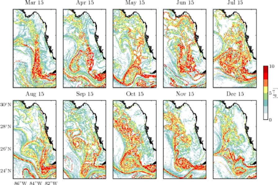
Figure 1 shows snapshots of FTLE field, which were computed using the software package MANGEN, a dynamical systems toolkit designed by F. Lekien that is available at http://www.lekien.com/francois/software/mangen. At each time the algorithm coded in MANGEN performs the following tasks. First, system (2) is integrated using a fourth-order Runge–Kutta–Fehlberg method for a grid of particles at time to get their positions at time , which are the values of the flow map at each point. This requires interpolating the velocity data, which is carried out employing a cubic method. Second, the spatial gradient of the flow map is obtained at each point in the initial grid by central differencing with neighboring grid points. Third, the FTLE is computed at each point in the initial grid by evaluating (1). The previous three steps are repeated for a range of values to produce a time series of FTLE field. Here we have set d so that the maximizing ridges of the FTLE fields shown in Figure 1 correspond to attracting LCSs. The choice d was suggested by the time it takes a typical fluid particle to leave the WFS domain. Clearly, some particles will exit the domain before 60 d of integration. In this case, MANGEN evaluates expression (1) using the position of each such particles prior exiting the domain. Note that due to the choice d the time series of computed FTLE fields based on our year-long record of simulated currents can only have a 10-month maximum duration.
The regions of most intense red tonalities in each panel of Figure 1 roughly indicate maximizing ridges of FTLE field. These regions are seen to form smooth, albeit highly structured, curves that constitute the desired LCSs or transport barriers. Of particular interest is the triangular-shaped area on the southern portion of the WFS with small FTLEs bounded by the western Florida coast on the east, the lower Florida keys on the south, and large maximizing ridges of FTLE field on the west. The latter constitute a cross-shelf transport barrier that approximately coincides in position with the western boundary of the FZ identified in Yang et al. (1999). This is most clearly visible during the period May through September. The sequence of snapshots of FTLE field in Figure 1 also reveals a seasonal movement of the cross-shelf transport barrier, being offshore during the winter and closer to the coast during the summer, which is in agreement with drifter observations (Morey et al., 2003).
4 LCSs Derived from Measured Currents
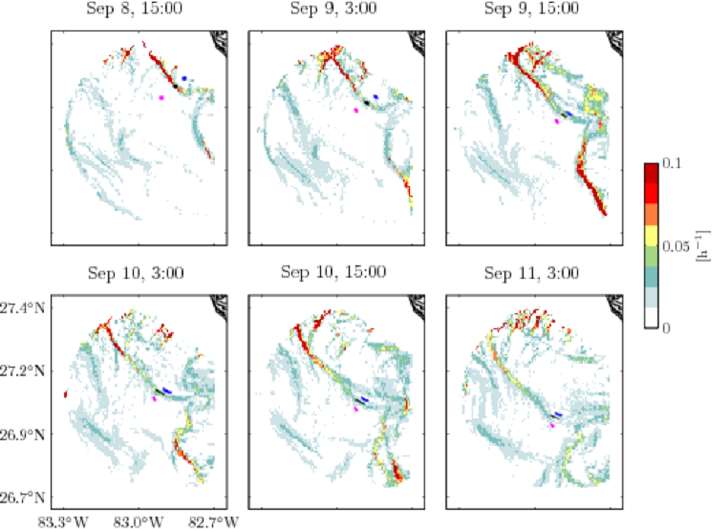
Figure 2 shows a sequence of snapshots of FTLE field computed using surface velocity inferred from HF radar measurements taken during September 2003 in an approximately 60 km 80 km domain on the WFS off Tampa Bay.
The HF radar measurements consist of measurements made with Wellen radars, which mapped coastal ocean surface currents over the above domain with 30-minute intervals (Shay et al., 2006). The computation of FTLEs was performed backward in time ( h) so that the maximizing ridges of FTLE field in Figure 2 indicate attracting LCSs, which are analogous to perturbed unstable invariant manifolds. The numerical computation of the FTLEs was not carried out using the MANGEN software package. Instead, we developed our own MATLAB codes, which, employing a methodology similar to that outlined in the previous section, allowed us to more easily handling FTLE computation based on velocity data defined on an irregular and totally open domain.
The transport barrier character of the attracting LCSs identified in the FTLE fields depicted in Figure 2 is illustrated by numerically simulating the evolution of three clusters of fluid particles. One of the clusters (black spot in the figure) is initially chosen on top of one LCS, while the other two clusters (dark-blue and magenta spots in the figure) are initially located at one side and the other of the LCS. Looking at the evolution of the clusters in time, we note that the black cluster remains on top of the LCS and stretches along it as time progresses. Also note that dark-blue and magenta clusters remain on two different sides, indicating the absence of flux across the LCS.
We remark that LCSs are identifiable in the region covered by the HF radar system through the whole month of September 2003. However, because of the limited domain of the radar footprint and the short deployment time window, we cannot say with certainty that any of the observed structures corresponds to the boundary of the FZ. In spite of this uncertainty, our analysis of the HF radar measurements is highly encouraging inasmuch as it demonstrates the feasibility of tracking the evolution of the boundary of the FZ in near real time.
5 Biological Implications
In addition to being an interesting physical feature whose underlying dynamics deserves further study, the cross-shelf transport barrier on the WFS also has potentially important biological implications.
The toxic dinoflagellate Karenia brevis has a rather restricted spatial distribution, primarily the GoM (Kusek et al., 1999). While K. brevis exists in low concentrations in vast areas of the GoM, it occasionally forms blooms along the northern and eastern coasts of the GoM (Wilson and Ray, 1956; Geesey and Tester, 1993; Tester and Steidinger, 1997; Dortch et al., 1998; Kusek et al., 1999; Magana et al., 2003). The largest and most frequent blooms, however, occur along the southern portion of the WFS (Steidinger and Haddad, 1981; Kusek et al., 1999). Where these occur, there can be widespread death of fish, manatees, dolphins, turtles, and seabirds as a result of the brevetoxins produced by K. brevis (Bossart et al., 1998; Landsberg and Steidinger, 1998; Landsberg, 2002; Shumway et al., 2003; Flewelling et al., 2005). The brevetoxins also end up in an aerosol, which affects human respiration (Backer et al., 2003; Kirkpatrick et al., 2004). Being slow growing while fast swimming algae (Chan, 1978; Brand and Guillard, 1981), dinoflagellates have the highest potential for achieving high population densities as a consequence of biophysical accumulation rather than actual growth. As a result of expatriate losses, K. brevis (and other dinoflagellates) would be expected to develop large blooms only in regions where stirring by currents is low. Indeed, many dinoflagellate blooms tend to occur in enclosed basins such as estuaries and lagoons, where expatriate losses are reduced. However, as mentioned above, K. brevis often forms large blooms along the open coastline of the southern portion of the WFS, typically inside the FZ.
We hypothesize that the cross-shelf transport barrier associated with the FZ provides a mechanism that reduces K. brevis expatriation. A corollary of this hypothesis is that this barrier allows the nutrients from land runoff to accumulate near the coastline rather than being swept away by currents. While we cannot explain why K. brevis often dominates over other species of dinoflagellates in the FZ, we can predict that slow growing dinoflagellates will be more prevalent within the FZ than outside.
6 Summary
In this letter we have shown that, when analyzed using dynamical systems methods, a year-long record of surface currents produced by a regional version of HYCOM reveals the presence of a cross-shelf transport barrier on the southern portion of the WFS, which is in approximately the same location as the boundary of the FZ identified earlier by Yang et al. (1999) using satellite-tracked drifter trajectories. The simulated cross-shelf transport barrier was robust, being present in all seasons while undergoing a seasonal oscillation. The simulated cross-shelf transport barrier was closer to shore in the summer months than in the winter months in agreement with observations (Morey et al., 2003). HF radar measurements were analyzed in a similar fashion and this analysis demonstrated the feasibility of experimentally monitoring transport barriers on the WFS using a system that can be operated in near real time.
Acknowledgements.
We thank I. Udovydchenkov for useful discussions. MJO was supported by NSF grant CMG-0417425 and PARADIGM NSF/ONR-NOPP grant N000014-02-1-0370. IAR, MGB, FJBV, and HK were supported by NSF grant CMG-0417425. LKS and the WERA HF Radar deployment and analyses were supported by ONR grant N00014-02-1-0972 through the SEA-COOS program administered by UNC-CH. The NOAA ACT program provided partial travel support for the WERA deployment personnel. We thank T. Cook, B. Haus, J. Martinez, and S. Guhin in deploying and maintaining the radar along the WFS.References
- Backer et al. (2003) Backer, L. C., et al. (2003), Recreational exposure to aerosolized brevetoxins during Florida red tide events, Harmful Algae, 2, 19–28.
- Bossart et al. (1998) Bossart, G. D., D. G. Baden, R. Y. Ewing, B. Roberts, and S. D. Wright (1998), Brevetoxicosis in manatees (Trichechus manatus Latirostris) from the 1996 epizoodic: gross, histopathologic and immunocytochemical features, Toxicol. Pathol., 26, 276–282.
- Brand and Guillard (1981) Brand, L. E., and R. R. L. Guillard (1981), The effects of continuous light and light intensity on the reproduction rates of twenty-two species of marine phytoplankto, J. Exp. Mar. Biol. Ecol., 50, 119–132.
- Chan (1978) Chan, A. T. (1978), Comparative physiological study of marine diatoms and dinoflagellates in relation to irradiance and cell size. I. Growth under continuous light, J. Phycol., 14, 396–402.
- Chassignet et al. (2006a) Chassignet, E. P., H. E. Hurlburt, O. M. Smedstad, G. R. Halliwell, P. J. Hogan, A. J. Wallcraft, R. Baraille, and R. Bleck (2006a), The HYCOM (HYbrid Coordinate Ocean Model) data assimilative system, J. Mar. Sys., in press.
- Chassignet et al. (2006b) Chassignet, E. P., H. E. Hurlburt, O. M. Smedstad, G. R. Halliwell, P. J. Hogan, A. J. Wallcraft, and R. Bleck (2006b), Ocean prediction with the HYbrid Coordinate Ocean Model (HYCOM), in Ocean Weather Forecasting: An Integrated View of Oceanography, edited by E. P. Chassignet and J. Verron, pp. 413–436, Springer.
- Dortch et al. (1998) Dortch, Q., C. Moncreiff, W. Mendenhall, M. Parsons, J. Franks, and K. Hemphill (1998), Spread of Gymnodinium breve into the northern Gulf of Mexico, in Harmful Algae, edited by B. Reguera, J. Blanco, M. L. Fernandez, and T. Wyatt, pp. 143–144, Xunta de Galicia and Intergovernmental Oceanographic Commission of UNESCO.
- Flewelling et al. (2005) Flewelling, L. J., et al. (2005), Brevetoxicosis: Red tides and marine mammal mortalities, Nature, 435, 755–756.
- Geesey and Tester (1993) Geesey, M., and P. A. Tester (1993), Gymnodinium breve: ubiquitous in Gulf of Mexico waters?, in Toxic Phytoplankton Blooms in the Sea, edited by S. T. J. and Y. Shimizu.
- Haller (2000) Haller, G. (2000), Finding finite-time invariant manifolds in two-dimensional velocity fields, Chaos, 10, 99–108.
- Haller (2001a) Haller, G. (2001a), Distinguished material surfaces and coherent structures in 3D fluid flows, Physica D, 149, 248–277.
- Haller (2001b) Haller, G. (2001b), Lagrangian structures and the rate of starin in a partition of two-dimensional turbulence, Phys. Fluids, 13, 3365–3385.
- Haller (2002) Haller, G. (2002), Lagrangian coherent structures from approximate velocity data, Physics Fluid, 14, 1851–1861.
- Haller and Yuan (2000) Haller, G., and G. Yuan (2000), Lagrangian coherent structures and mixing in two-dimensional turbulence, Physica D, 147, 352–370.
- Kirkpatrick et al. (2004) Kirkpatrick, B., et al. (2004), Literature review of Florida red tide: Implications for human health effects, Harmful Algae, 3, 99–115.
- Kusek et al. (1999) Kusek, K. M., G. Vargo, and K. Steidinger (1999), Gymnodinimum breve in the field, in the lab, and in the newspaper-a scientific and journalistic analysis of Florida red tides, Contri. Mar. Sci., 34, 1–229.
- Landsberg (2002) Landsberg, J. H. (2002), The effects of harmful algal blooms on aquatic organisms, Rev. Fish. Sci., 10, 113–390.
- Landsberg and Steidinger (1998) Landsberg, J. H., and K. A. Steidinger (1998), A historical review of Gymnodinium breve red tides implicated in mass mortalities of the manatee (Trichechus manatus Latirostris) in Florida, USA, in Harmful Algae, edited by B. Reguera, M. L. Fernandez, and T. Wyatt, pp. 97–100, Xunta de Galicia and Intergovernmental Oceanographic Commission of UNESCO.
- Lekien et al. (2005) Lekien, F., C. Coulliette, A. J. Mariano, E. H. Ryan, L. K. Shay, G. Haller, and J. E. Marsden (2005), Pollution release tied to invariant manifolds: A case study for the coast of Florida, Physica D, 210, 1–20.
- Magana et al. (2003) Magana, H. A., C. Contreras, and T. A. Villareal (2003), A historical assessment of Karenia brevis in the western Gulf of Mexico, Harmful Algae, 2, 163–171.
- Morey et al. (2003) Morey, S. L., P. J. Martin, J. J. O’Brien, A. A. Wallcraft, and J. Zavala-Hidalgo (2003), Export pathways for river discharged fresh water in the northern Gulf of Mexico, J. Geophys. Res., 108(C10), 3303, 10.1029/2002JC001674.
- Shadden et al. (2005) Shadden, S. C., F. Lekien, and J. E. Marsden (2005), Definition and properties of Lagrangian coherent structures from finite-time Lyapunov exponents in two-dimensional aperidic flows, Physica D, 212, 271–304.
- Shay et al. (2006) Shay, L. K., J. Martinez-Pedraja, T. M. Cook, B. K. Haus, and R. H. Weisberg (2006), Surface current mapping using Wellen radars, J. Atmos. Oceanogr. Thech. , in press.
- Shumway et al. (2003) Shumway, S. E., S. M. Allen, and P. D. Boersma (2003), Marine birds and harmful algal blooms: sporadic victims or under-reported events?, Harmful Algae, 2, 1–17.
- Steidinger and Haddad (1981) Steidinger, K. A., and K. Haddad (1981), Biologic and hydrographic aspects of red-tides, BioScience, 31, 814–819.
- Tester and Steidinger (1997) Tester, P. A., and K. A. Steidinger (1997), Gymnodinium breve red tide blooms: Initiation, transport, and consequences of surface circulation, Limnol. Oceanogr., 42, 1039–1051.
- Wilson and Ray (1956) Wilson, W. B., and S. M. Ray (1956), The occurrence of Gymnodinium breve in the western Gulf of Mexico, Ecol., 37, 388.
- Yang et al. (1999) Yang, H., R. H. Weisberg, P. P. Niiler, W. Sturges, and W. Johnson (1999), Lagrangian circulation and forbidden zone on the West Florida Shelf, Cont. Shelf. Res., 19, 1221–1245.