Possibility of Turbulence from a Post-Navier-Stokes Equation

Abstract

We introduce corrections to the Navier-Stokes equation arising from the transitions between molecular states and the injection of external energy. In the simplest application of the proposed post Navier-Stokes equation, we find a multi-valued velocity field and the immediate possibility of velocity reversal, both features of turbulence.

I Introduction

Traditionally, any attempt to describe turbulent behavior in fluids starts with the Navier-Stokes equation (NSE) Frisch (1995). However, success has at best been mixed Deissler (1984). In this Letter, we explore the idea that NSE is not the unique approach to the study of turbulence, and that turbulence may be found in what we label as post-Navier-Stokes equations. What could modify NSE? In our opinion, the molecular nature of fluids can no longer be ignored Nerushev and Novopashin (1996, 1997); Novpashin (2002); Novopashin and Muriel (1998); Hinkle and Muriel (2005, to be published). So we attempt to modify NSE by including quantum concepts, and in particular, in its simplest application, arrive at the possibility of velocity reversal and multi-valued velocity fields Sirovich (1991), both important features of turbulence. Before showing these final results, we need to make two comments on the derivation of NSE to justify our proposed post-NSE.

The traditional way of deriving the Navier-Stokes equation (NSE) is phenomenological, based on the continuum model and conservation of momentum. It may also be derived using the kinetic theory of structureless molecules by starting with the Boltzmann transport equation

$$\left(\frac{\partial}{\partial t}+\frac{p_{i}}{m}\frac{\partial}{\partial x_{i}}+F_{i}\frac{\partial}{\partial p_{i}}\right)f(r,p,t)=\left[\frac{\partial f(r,p,t)}{\partial t}\right]_{\mbox{\small\em coll}},$$ (1)

where we follow the conventional definitions from Huang Huang (1963). For the purpose of differentiating our approach to arrive at post-NSE equations, we quickly comment on the assumptions of the derivation.

First, collisional invariants $\chi$ are defined such that

$$\int\mathrm{d}^{3}p\,\chi(r,p)\left[\frac{\partial f(r,p,t)}{\partial t}\right]_{\mbox{\small\em coll}}=0.$$ (2)

These collisional invariants are $\chi=m$ (mass), $\chi=mv_{i}$ ($i=1,2,3$ momentum), $\chi=\frac{1}{2}m|v-u(r,t)|^{2}$ (thermal energy), where $u(r,t)=\langle v\rangle$.

To get the NSE, multiply the Boltzmann transport equation by $p$ and integrate over all momentum, yielding

$$\rho\left(\frac{\partial}{\partial t}+u\cdot\nabla\right)u=\frac{\rho}{m}F-\nabla\cdot P$$ (3)

where $\rho(r,t)=mn(r,t)$ and $P_{ij}=\rho\langle(v_{i}-u_{i})(v_{j}-u_{j})\rangle$. Our first comment is that the above equation results from microscopic conservation laws assuming elastic collisions of point molecules.

To arrive at the traditional NSE, we need an explicit form of the pressure tensor, which is taken to be

$$P_{ij}=\delta_{ij}P-\mu\left[\left(\frac{\partial u_{i}}{\partial x_{j}}+\frac{\partial u_{j}}{\partial x_{i}}\right)-\frac{2}{3}\delta_{ij}\nabla\cdot u\right]$$ (4)

where $\mu$ is the viscosity. The above choice of the pressure is justified by the assumption that a fluid element, or microscopically, as our second comment, the particle of the model has no intrinsic angular momentum.

In full component form, the Navier-Stokes equation is

$$\rho\left(\frac{\partial}{\partial t}+u_{j}\frac{\partial}{partialx_{j}}\right)u_{i}=\frac{\rho}{m}F_{i}$$ (5)

$$-\frac{\partial}{\partial x_{j}}\left(\delta_{ij}P-\mu\left[\left(\frac{\partial u_{i}}{\partial x_{j}}+\frac{\partial u_{j}}{\partial x_{i}}\right)-\frac{2}{3}\frac{\partial u_{j}}{\partial x_{i}}\right]\right).$$

Notice that before the introduction of the definition of the pressure, the conservation of momentum equation is exact in so far as the Boltzmann transport equation is valid. This equation comes only from the left-hand side of the Boltzmann equation. The contribution from the collision term disappears by virtue of conservation of momentum and the assumption of elastic collisions. Hence, only the left hand side of the Boltzmann transport equation is important to yield the conservation of momentum equation and NSE. We stress the two assumptions needed to arrive at the Navier-Stokes equation: first, elastic collisions, and second, the absence of angular momentum of the structureless molecules. What will happen if these two assumptions are no longer valid?

II Correcting the Navier-Stokes Equation

Suppose that each of the molecules could be found in any one of $N$ states, the ground state and $(N-1)$ excited states. Assume that excitations and de-excitations are induced by molecular collisions, which are now inelastic. Then the semi-classical analogue of the Boltzmann transport equation for each of $N$ distribution functions will be

$$\left(\frac{\partial}{\partial t}+\frac{p_{i}}{m}\frac{\partial}{\partial x_{i}}+F_{i}\frac{\partial}{\partial p_{i}}\right)f_{n}(r,p,t)=$$ (6)

$$\left[\frac{\partial f_{n}(r,p,t)}{\partial t}\right]_{\mbox{\small\em inelastic}},$$

where the collision term might be replaced by

$$\left[\frac{\partial f_{n}(r,p,t)}{\partial t}\right]_{\mbox{\small\em inelastic}}=\sum_{m\neq n}^{N}\gamma_{mn}Jf_{m}(r,p)$$ (7)

$$-\sum_{m\neq n}^{N}\gamma_{nm}Jf_{n}(r,p)+\sigma Kf_{n}(r,p)$$

$\gamma_{mn}$ is the transition probability of a particle in the $m$ state jumping to the $n$ state. $J$ is a “jump” operator that will carry the conservation law the we will invoke in the time evolution of $N$ distribution probabilities. $K$ is a “kick” operator that allows the injection of energy from outside Muriel (1998, 2002a, 2003, 2002b). $\sigma$ is the probability that a particle is kicked to a different momentum by external means. The kick operator makes the injection of energy into the system possible. Eq. (6) is a generalization of our previous models Muriel (1998, 2002a, 2003, 2002b).

To calculate macroscopic averages, not only must we integrate over all momentum, we should also sum over all $N$ states, to yield

$$\rho\left(\frac{\partial}{\partial t}+u\cdot\nabla\right)u=\frac{\rho}{m}F-\nabla\cdot P+\mathit{driving}+\mathit{radiative},$$ (8)

where

$$\mathit{driving}=\sigma\sum_{n=1}^{N}\int\mathrm{d}p^{3}pKf_{n}(r,p),$$ (9)

$$\mathit{radiative}=$$ (10)

$$\sum_{n=1}^{N}\int\mathrm{d}p^{3}p\left[\sum_{m\neq n}^{N}\gamma_{mn}Jf_{m}(r,p)-\sum_{m\neq n}^{N}\gamma_{nm}Jf_{n}(r,p)\right].$$

We may think of (9) and (10) as the quantum corrections to the NSE. The first sum (9) is the driving term. We will call the second sum (10) the radiative correction because every transition is accompanied by radiation. (NSE ignores not only molecules, but also photons.) The radiative term represents the contribution of the internal degrees of freedom of molecules to the macroscopic flow of a fluid. If all the transition probabilities are zero, we simply reproduce the classical NSE. This last equation, our post-NSE, no longer assumes elastic collisions and the absence of angular momentum of the particles. The operators $J$ and $K$ have been defined in our earlier model calculations Muriel (1998, 2002a, 2003, 2002b), they may be redefined with new models, but we will simplify them to show that even the simplest application of Equation (8) leads to novel results.

We have had occasions to consider the radiative term Muriel (1998, 2002a, 2003, 2002b), and will consider them later even more, but for now to arrive at immediate new results, we consider only the influence of quantized kicks defined by the operator $Kf_{n}(r,p)=f_{n}(r,p-\Pi)$ yielding

$$\int\mathrm{d}p^{3}pKf_{n}(r,p)=mu+n(r,t)\Pi.$$ (11)

III Examples

Remove the force $F$ and drop the divergence of the pressure to obtain a non-linear equation in one dimension

$$frac{\partial u}{\partial t}+\frac{1}{2}\frac{\partial u^{2}}{\partial x}-\sigma u=\frac{\sigma\Pi}{m}.$$ (12)

It is the simplest application of our post-NSE but which remains a challenge still.

The stationary solution is to be obtained from

$$\frac{1}{2}\frac{\partial u^{2}}{\partial x}-\sigma u=\frac{\sigma\Pi}{m},$$ (13)

which is

$$u(x)=-\frac{\Pi}{m}\left[W_{k}\left(-\frac{m}{\sigma\Pi}\mathrm{e}^{-\frac{m\sigma}{\Pi}(x+C)-1}\right)+1\right]$$ (14)

where $C$ is a constant and $W_{k}$ denotes the $k^{\mathrm{th}}$ branch of the Lambert W function. The function $W_{k}(z)$ is a solution of the equation $w\mathrm{e}^{w}=z$ in the complex plane Corless et al. (1996). The Lambert W function is multi-valued, making the stationary average velocities multi-valued.

We will choose a toroidal geometry, and put $x=L\sin(2\pi\theta)$, $\theta=0,\ldots 1$, to ensure periodic boundary conditions. The physical model is one-dimensional, a donut of circumference $2\pi L$. One could imagine a paddlewheel half-stuck into the donut to provide quantum kicks to the fluid. If $u(\theta=0)=0$, then $C=-\frac{\Pi}{\sigma m}\ln\Pi$ and we get

$$u_{k}(\theta)=-\frac{\Pi}{m}\left[W_{k}\left(-\frac{m}{\sigma}\ mathrm{e}^{-\frac{m\sigma}{\Pi}L\sin(2\pi\theta)-1}\right)+1\right].$$ (15)

We plot $u_{k}(\theta)$ in Figure 1 for for $k=0,\pm 1,\ldots\pm 5$.

Real part	Imaginary Part

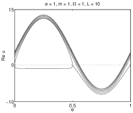
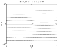
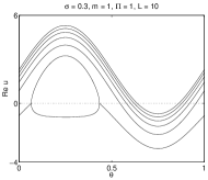
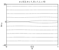
Figure 1: Average velocity as a function of the angle for the torus geometry. The principal branch is complemented by the other branches which almost form a continuum.

Using the method of characteristics, we now find the transient solutions of

$$\frac{\partial u}{\partial t}+\frac{1}{2}\frac{\partial u^{2}}{\partial x}-\sigma u=\frac{\sigma\Pi}{m},\quad u(x,0)=f(x),$$ (16)

where $f(x)$ are the initial velocity averages. Rewriting (16) as $u\frac{\partial u}{\partial x}+\frac{\partial u}{\partial t}=\sigma u+\frac{\sigma\Pi}{m}$, we identify its characteristic equations,

$$x^{\prime}(\tau)=u(\tau),\quad t^{\prime}(\tau)=1,\quad u^{\prime}(\tau)=\sigma u(\tau)+\frac{\sigma\Pi}{m}.$$ (17)

The boundary conditions can be parameterized as

$$x_{0}(s)=s,\quad t_{0}(s)=0,\quad u_{0}(s)=f(s).$$ (18)

For each fixed value of $s$, solving the characteristic equations (17) with initial values $x(0;s)=x_{0}(s)$, $t(0;s)=t_{0}(s)$, $u(0;s)=u_{0}(s)$ yields a characteristic curve $u(x(\tau;s),t(\tau;s))$ in the solution surface $u(x,t)$. For more on the method of characteristics, see for example Guenther and Lee (1988).

The solution $u(x,t)$ is

$$u(x,t) = \mathrm{e}^{\sigma t}\left(\frac{\Pi}{m}+f(s)\right)-\frac{\Pi}{m},$$ (19)

$$x = s+f(s)\frac{\mathrm{e}^{\sigma t}-1}{\sigma}+\frac{\Pi}{m\sigma}(\mathrm{e}^{\sigma t}-\sigma t-1),$$ (20)

where $s$ is defined implicitly by the second equation. While it is not in general possible to express $u(x,t)$ explicitly, we can still interpret the solution in terms of the characteristic curves $u(x(t;s),t)$.

Depending on the problem parameters $\sigma$, $m$, $\Pi$, and $f(x)$, it is possible that the characteristic curves cross. If the characteristics cross at $(x_{c},t)$, then there are multiple curves $s_{1},s_{2},\ldots$ such that $x_{c}=x(t;s_{1})=x(t;s_{2})=\cdots$. Moreover, the solution permits multiple values $u(x_{c},t)=u(x(t;s_{1}),t),u(x(t;s_{2}),t),\ldots$ at the crossing point. Figure 2 demonstrates this feature in a simple example.

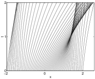
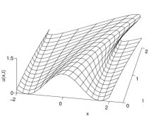
Figure 2: The transient problem with $\sigma=0.1$, $m=1$, $\Pi=1$, and $f(x)=\cos(x)^{2}$. Left: The characteristics cross at about $t=1$. Right: The solution surface $u(x,t)$ folds on itself and becomes multi-valued where the characteristics cross.

IV Conclusions

It appears that in our first applications of a highly simplified post-Navier-Stokes equation, we have arrived at multi-valued velocities as a function of location. They may well be interpreted as possible states of a turbulent system from which transitions to other states may be possible. The possibility of velocity reversal, a feature of turbulence, is immediately obvious. This result seems to be the first instance of an analytic derivation of a multi-valued velocity field and deserves further studies.

References

- Frisch (1995) U. Frisch, The Legacy of A. N. Kolmogorov (Cambridge University Press, New York, 1995).
- Deissler (1984) R. G. Deissler, Rev. Mod. Phys 56, 223 (1984).
- Nerushev and Novopashin (1996) O. Nerushev and S. Novopashin, JETP Lett. 64, 47 (1996).
- Nerushev and Novopashin (1997) O. Nerushev and S. Novopashin, Phys. Lett. A 232, 243 (1997).
- Novpashin (2002) S. Novpashin, in Engineering Turbulence Modeling and Experiments, edited by W. Rodi and N. Fueyo (Elsevier, Amsterdam, 2002), 5.
- Novopashin and Muriel (1998) S. Novopashin and A. Muriel, JETP Lett. 68 (1998).
- Hinkle and Muriel (2005) L. Hinkle and A. Muriel, J. Vac. Sci. Technol. A 23, 4 (2005).
- Hinkle and Muriel (to be published) L. Hinkle and A. Muriel, J. Vac. Sci. Technol. A (to be published).
- Sirovich (1991) L. Sirovich, New Perspectives in Turbulence (Springer Verlag, New York, 1991).
- Huang (1963) K. Huang, Statistical Mechanics (Wiley, New York, 1963).
- Muriel (1998) A. Muriel, Physica D 124, 225 (1998).
- Muriel (2002a) A. Muriel, Physica A 305, 379 (2002a).
- Muriel (2003) A. Muriel, Physica A 322, 139 (2003).
- Muriel (2002b) A. Muriel, in Coherent Structures in Complex Systems, edited by L. Reguerram, J. Bonilla, and J. Rubi (Springer-Verlag, Berlin, 2002b).
- Corless et al. (1996) R. Corless, G. Gonnet, D. Hare, G. Jeffrey, and D. Knuth, Adv. Comp. Math 5, 329 (1996).
- Guenther and Lee (1988) R. Guenther and J. Lee, Differential Equations of Mathematical Physics and Integral Equations (Dover, New York, 1988).