Hölder-exponent-MFDFA-based test for long-range correlations in pseudorandom sequences

Abstract

We discuss the problem for detecting long-range correlations in sequences of values obtained by generators of pseudo-random numbers. The basic idea is that the Hölder exponent for a sufficiently long sequence of uncorrelated random numbers has the fixed value $h=1/2$. The presence of long-range correlations leads to deviation from this value. We calculate the Hölder exponent by the method of multifractal detrended fluctuation analysis (MFDFA). We discuss frequently used tests for randomness, finite sample properties of the MFDFA, and the conditions for a correct application of the method. We observe that the fluctuation function $F_{q}$ used in the MFDFA reacts to trends caused by low periodicity presented in the pseudo-random number generator. In order to select appropriate generators from the numerous programs we propose a test for the ensemble properties of the generated pseudo-random sequences with respect to their robustness against presence of long-range correlations, and a selection rule which orders the generators that pass the test. Selecting generators that successfully pass the ensemble test and have good performance with respect to the selection rule is not enough. For the selected generator we have to choose appropriate pseudo-random sequences for the length of the sequence required by the solved problem. This choice is based on the closeness of the Hölder exponent of the generated sequence to its value $1/2$ characteristic for the case of absence of correlations.

1 Pseudorandom sequences, Hölder exponent and multifractal detrended fluctuation analysis

Computer random number generators have many applications in physics as for an example in the Monte Carlo methods [1, 2] or in the nonlinear time series analysis [3, 4]. Computers implement deterministic algorithms, hence they are not able to generate sequences of truly random numbers. Thus the randomness of the sequences is relative: What can be random enough for one application may not be random enough for another application. The computer generated sequences are called pseudorandom, and in order to be appropriate for scientific applications they have to satisfy many requirements and must pass extensive statistical tests. For an example the period of the generator (the number of different results before the generator repeats itself) must be as large as possible. Another requirement is that the generated numbers should not be correlated among themselves. A significant class of such correlations are the long-range correlations which decay much slower than exponentially with time or distance and are observed in many systems in the Nature [5, 6]. The autocorrelation function $c_{n}=\langle\eta_{i}\eta_{i+n}\rangle$ of a pseudorandom sequence $\{\eta_{\alpha}\}$ ideally should be a Kronecker $\delta_{n,0}$. $c_{n}$ is not a convenient tool for detecting long-range correlations among the numbers in the sequence since the presence or absence of weak correlation at large $n$ is usually masked by statistical fluctuations. Hence we have to apply a separate test to detect them. In this paper we propose such a test which is based on the simple fact that the Hölder exponent for the sequence of uncorrelated random numbers has the fixed value of $1/2$ (for more details see the Appendix). The deviation from this value for large $n$ is evidence for possible long-range correlations in the sequences generated by the used pseudo-random numbers generator.

The Hölder exponent is a measure of irregularity of a curve at a singular point [7, 8]. Let us consider a function $z(t)$. Its $\tau$-oscillation at value $t$ is

(1) $${\rm osc}_{\tau}(t)=\sup_{\mid t-t^{\prime}\mid\leq\tau}\hskip 2.84544ptz(t^{\prime})-\inf_{\mid t-t^{\prime}\mid\leq\tau}\hskip 2.84544ptz(t^{\prime}).$$

The graph of $z(t)$ is fractal if ${\rm osc}_{\tau}(t)/\tau\to+\infty$ uniformly with respect to $t$. For differentiable $z(t)$ the ratio ${\rm osc}(t)/(2\tau)$ tends to $dz/dt$ for $\tau\to 0$. When the limes superior of the ratio is infinite, there is no derivative, and the Hölder exponent measures the singularity of the graph of $z(t)$ in this point. A function $z(t)$ is Hölderian of exponent $h$ if a constant $c$ exists such that for all $t^{\prime}$

(2) $$\mid z(t)-z(t^{\prime})\mid\leq c\mid t-t^{\prime}\mid^{h}$$

or in terms of $\tau-$oscillations ${\rm osc}_{\tau}(t)\leq c\tau^{h}$. If ${\rm osc}_{\tau}(t)\geq c\tau^{h}$ the function $z(t)$ is anti-Hölderian of exponent $h$ at the point $t$. The relation between $c_{n}$ and the Hölder exponent for the case of Hurst noise is discussed in the Appendix. We recall from there the relationship (for large $n$)

(3) $$c_{n}=h(2h-1)n^{2h-2}.$$

For the case of pure white noise ($c_{n}=0$), $h=1/2$. When $h>1/2$, $c_{n}>0$, i.e., the series of data are correlated and when $h<1/2$, $c_{n}<0$, i.e., the data series are anti-correlated.

We shall calculate the Hölder exponent for our pseudorandom sequences by means of the MFDFA method [9] which is briefly described in the Appendix. We perform all calculations by means of the MFDFA(1),i.e., linear fit of the trend in each segment (When the fit is made by polynomial of $p$-th order the method is denoted as MFDFA(p)). Our choice $p=1$ respects the fact that no trend is to be expected in the investigated sequences of numbers. Below we shall discuss a test for long-range correlations and not for a trend in the generated sequences of pseudorandom numbers. If such a trend exists it has to be detected by other tests. But even in the case when these additional tests are not performed the MFDFA reacts to the presence of trends and nonstationarities. This sensitivity is know to exist for DFA [10, 11] and as we shall observe below it exists for the case of MFDFA too.

We use as random number generators several generators from [12] namely ran0, ran2, ran3, a quick and dirty generator which we call qdg as well as the generator based on the program G05CAF from the NAG library. ran0 is the minimal standard generator which has to be satisfactory for most applications but if its parameters are not appropriately chosen the generator can have correlations. The generator ran2 is claimed to be very good one and without serial correlations up to limits of its floating point precision. ran3 is based on the algorithm due to Knuth [13]. qdg is based on a cycle containing the lines of code

$\dots$

jran=mod(jran*ia+ic,im)

ran=float(jran)/float(im)

$\dots$

where im, ia, ic are appropriately chosen parameters. The above generators are not tested and compared with respect of long-range correlations.

The paper is organized as follows. In the following section we discuss the properties of the investigated generators with respect for standard tests for randomness. Finite sample properties of the MFDFA method are investigated in section III in order to select interval of appropriate values for the parameter $q$ of the method for which the test for randomness has to be performed. In the section IV the behavior of the fluctuation function of the MFDFA method is discussed for the investigated generators and it is shown that the fluctuation function is a good indicator for deviation from fractality and presence of trends in the generators. In section V we discuss an ensemble test for long-range correlations in the random number generators as well as rules for selection of (i) most appropriate generator for the required length of the sequence and (ii) most appropriate sequences generated by a selected generator. Some concluding remarks are summarized in the last section where we discuss MFDFA(0) and MFDFA(1) with respect to their sensitivity to detect deviations from the case $h=1/2$. In the Appendix we describe shortly the relationship between the correlation function and the Hölder exponent as well as the MFDFA method.

2 Behavior of generators with respect to standard tests

In order to be sure that ran0, ran2, ran3, qdg and G05CAF produce sequences close to random ones we have tested them by standard tests such as a frequency test or a serial correlations test [1]. The general difficulty with statistical test on finite sequences lies in the statistical fluctuations. For the latter tests they are perfectly known. We expect that the generators generate sequences of pseudorandom numbers with histograms uniform in some interval ( $[0,1]$ for ran0, ran2, ran3, G05CAF and $[-1,1]$ for qdg). In order to perform the frequency test we sort a generated sequence of $N$ numbers into $B$ bins with expected mean value of the numbers in each bin $\overline{M}=N/B$. If the actual number of random numbers in the $j-$th bin is $M_{j}$ we can construct the quantity

(4) $$\chi^{2}_{\nu}=(1/\nu)\chi^{2}=(1/\nu)\{\sum_{j=1}^{B}[(M_{j}-\overline{M})^{2}/\overline{M}]\}$$

with $\nu=B-1$ degrees of freedom. $\chi^{2}_{\nu}$ must be different from $0$ because of presence of some fluctuations in a histogram of a finite sequence of numbers. However the value of $\chi_{\nu}^{2}$ must be not too large because large values are the evidence for the concentration of numbers in some bins and thus the generator is not random. $\chi^{2}$ was calculated for $\nu=49$ degrees of freedom and for a good random number generator $\chi^{2}$ has the value of about $40$ for a sequence of 50000 pseudorandom numbers. Characteristic values for the investigated generators are presented in Table I. We note (i) the good performance of the quick and dirty generator qdg for small length of the generated pseudorandom sequences opposite to the case of large length of the sequence and (ii) the fact that the different generators have different performance for different lengths of the sequence. We can conclude that all generators except the qdg passed this test and we observe that the choice of the appropriate generator depends on the lengths of the pseudorandom sequence we need.

As a second test we have calculated the autocorrelation at lag $\nu$

(5) $$c_{\nu}=\frac{1}{\sigma^{2}}\langle(x_{n}-\langle x\rangle)(x_{n-\nu}-\langle x\rangle)\rangle$$

where $\langle x\rangle$ and $\sigma^{2}$ are the mean and the variance of the sequence. Several typical results for the investigated generators are presented in Table II. The small values of the autocorrelations show that the generators successfully pass this test. This fact supports the observation that the long-range correlations could be quite good masked so that the pseudorandom number generators with such correlations could pass the standard correlation tests. We can conclude that except for the cases of very inappropriate generators the standard tests do not supply us with much information about the question if the pseudorandom generator we want to use is free from long-range correlations. We have to design other tests to detect such correlations. The test and rules which are discussed below are based on the use of the Hölder exponent which is calculated by means of the multifractal detrended fluctuation analysis (MFDFA) method.

3 Finite sample properties of MFDFA

Before we apply the MFDFA method to our pseudorandom number sequences we have to understand its finite sample properties. For infinite uncorrelated sequences of values the Hölder exponent has the fixed value $h=1/2$. We discuss here in detail finite sample properties of sequences generated by two of the generators: the generator ran2 which is claimed to be quite good in [12], and the generator ran0. The investigation of sequences generated by C05CAF and ran3 leads to the same conclusions. We estimate the Hölder exponent $h(q)$ from a sample of length $N$ for ensemble of pseudorandom sequences (For the role of the parameter $q$ see the Appendix ). The MFDFA method will be consistent when $h(q)\to 1/2$ with increasing length $N$ of the sample, and unbiased when the ensemble average $\langle h_{(N)}(q)\rangle\to 1/2$. Our observation is that the MFDFA method is consistent but biased for large $\mid q\mid$. For the investigation of the finite sample properties of the two generators we have used at least 10 ensembles each of $25$ random sequences (i.e. at least 250 different sequences). For larger number of sequences in the ensembles the results for $h(q)$ do not change significantly and the only significant effect is the decreasing of the standard deviation of the mean. We test the consistency of the method by keeping parameters unchanged except for the length of the time series which is increased . Several characteristic results for the generator ran0 are presented in Fig. 1. These results as well the results from other similar calculations starting from different seeds of the generator parameter idum of ran2 show that the MFDFA method is consistent. However, the method is biased for large $\mid q\mid$ as it can be seen from Fig. 1 and Fig. 2. We observe that for small $\mid q\mid$ (the numerical experiments lead us to the conclusion that small is $\mid q\mid\leq 2$) $h(q)$ stays around $0.5$ but for larger $\mid q\mid$ significant deviations exist (i) when we increase the length of the sequence and keep $s_{mix}$ and $s_{max}$ constant (Fig.1), and (ii) when we keep the length of the sequence constant and increase $s_{max}$ (Fig. 2). A part of the bias of the method for large $\mid q\mid$ can be removed by increasing sample size because for small sample size we have limited number of values with low probability. Nevertheless our advice is that all test for long-range correlations must be performed for small $\mid q\mid$. As generators generate only pseudorandom sequences we can not expect to obtain exactly $1/2$ as a value for $h$. Our numerical investigation has shown that differences of $0.005$ are admissible, i.e., the generator (from the point of view of ensembles of generated sequences) can be considered safe with respect to long range correlations when for small $\mid q\mid$ (between $0$ and $2$) its ensemble $h(q)$ spectrum is between $0.495$ and $0.505$.

4 Behavior of the fluctuation function

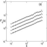
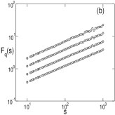
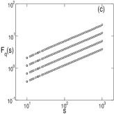
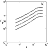
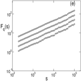
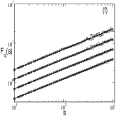
Figure 3: Fluctuation function $F_{q}(s)$ for the pseudorandom sequences from ran2 and ran0. From bottom to the top at each panel the lines are for $q=2,4,6,8$. Panels (a)-(c): Results for ran2, idum=2. Panel (a): Fluctuation functions for a sequence of $10^{4}$ points. The values of the Hölder exponent are: $h=0.505\pm 0.002$ ($q=2$); $h=0.505\pm 0.004$ ($q=4$); $h=0.503\pm 0.004$ ($q=6$); $h=0.499\pm 0.005$ ($q=8$). Panel (b): Fluctuation function for a sequence of $10^{5}$ points. $h=0.499\pm 0.001$ ($q=2$); $h=0.501\pm 0.001$ ($q=4$); $h=0.505\pm 0.002$ ($q=6$); $h=0.509\pm 0.003$ ($q=8$). Panel (c): Fluctuation function for a sequence of $10^{6}$ points. $h=0.500\pm 0.0004$ ($q=2$); $h=0.502\pm 0.001$ ($q=4$); $h=0.504\pm 0.001$ ($q=6$); $h=0.506\pm 0.001$ ($q=8$). Panel (d): Fluctuation function for ran0 with parameters $a=343$, $q=127773$, $r=2836$, $m=aq+r=43828975$ . Period of the generator is $4880$, idum=2. Panel (e): Fluctuation function for random number generator ran0 with parameters $a=16807$, $q=127773$, $r=2836$, $m=aq+r=2147483647$. idum=2, sequence of $10^{6}$ values. $h=0.511\pm 0.003$ for $q=2$; $h=0.506\pm 0.003$ for $q=4$; $h=0.501\pm 0.002$ for $q=6$; $h=0.498\pm 0.002$ for $q=8$. $a=16807$, $q=127773$, $r=2836$, $m=aq+r=2147483647$ for ran0. Panel (f): Comparison between fluctuation functions for sequences generated by the generators ran0 and ran2. Length of the sequences $10^{5}$ points. idum=2 for the two generators. Parameters of the generators $a=16807$, $q=127773$, $r=2836$, $m=aq+r=2147483647$ for ran0. Circles: Fluctuation functions for ran2. Squares: Fluctuation functions for ran0. Solid lines: Power-law fits for the sequence generated by ran2. From bottom to the top: $q=2,4,6,8$.

When we investigate sequences from a pseudo-random numbers generator first of all we have to check if the fluctuation function $F_{q}(s)$ from the MFDFA method really scales as a power of $s$ for different values of $q$. We expect $F_{q}(s)$ to be a straight line on the log-log scale (panels (a),(b),(c)) of Fig.3) . Deviations from this behavior are evidence for a problem. In panel (d) we see a broken line with a break point approximately at $1/2$ of the period of generator which is characteristic for sequences with periodic trend. Hence the MFDFA method reacts on trends in the generated sequences i.e. it can be used as a warning message for presence of trends too. In addition, even if the fluctuation function is a straight line, but the value of $h$ is significantly different from $0.5$ for small $\mid q\mid$, this is an evidence for presence of long-range correlations in the sequence of pseudo-random numbers. In panels (a)-(c) of Fig. 3 we observe that with increasing length of the sequence for ran2 $F_{q}(s)$ comes closer to a straight line. This could be expected because the larger length leads to a better statistics as the form of the sequence histogram approaches the ideal assumed histogram form. Panel (f) shows a comparison between fluctuation functions for characteristic sequences generated by ran0 and ran2. We observe that ran2 is more robust than ran0 with respect to long-range correlations because the fluctuation function lines for different $q$ are closer to straight lines for the case of the generator ran2 for all range of segment lengths $s$. Fluctuation functions for ran0 are more dispersed for large lengths of the segment $s$.

We haven’t obtained satisfactory results for the generator qdg. This means that the fluctuation function does not scale as power law of the length of the segment (as in the case of the vales of im=$6075$, ia=$106$, ic=$1283$), or the scaling exponent is quite significant from $0.5$ as for an example in the case of the values of parameters im=$233280$, ia=$9301$, ic=$49297$.

5 A test and selection rules

On the basis of obtained results we can formulate a test and rules of selection among pseudo-random numbers generators and among sequences generated by a generator. The test determines the conditions under which a random number generator can be considered to generate large amount of sequences free from long-range correlations. We note here that no absolute test exists, i.e., a generator can be good for one required length of the sequence but another generator could be better for another length of the sequence. Let us have several pseudo-random numbers generators and let us want to choose these of them which generate large amount of sequences free of long-range correlations. This choice can be made on the basis of the following test on the ensembles of pseudorandom sequences.

For a given random number generator take at least 10 different ensembles each of at least 25 pseudorandom sequences and calculate the Hölder exponent by means of MFDFA(1) method for $\mid q\mid\leq 2$. If for all ensembles the fluctuation function $F_{q}(s)$ scales as power law for all $q$ and the Hölder exponent is between $0.495$ and $0.505$ the random number generator can be considered to be able to generate large amount of sequences free from long-range correlations.

Generators which pass the above test have to be preferred with respect to generators that fail the test. Thus one can select generators with small probability of generating sequences possessing long-range correlations (for the required length of the sequence). The next question which arises is how to order the appropriate generators and to select one of them. The answer is given by a selection rule which is based on a power-law scaling property of the fluctuation function and on closeness of corresponding Hölder exponent to $1/2$ and states

Let us have two pseudo-random numbers generators which pass the above test. Let us calculate the fluctuation function $F_{q}(s)$ for at least 10 different ensembles each of at least $25$ sequences for the two generators. The generator which has closer to power law form of $F_{q}(s)$ for all $q$ and for which the $h(q)$ is closer to $1/2$ is more robust with respect to long-range correlations.

An extensive investigation leaded us to the following ranking of the generators with respect of the test and the selection rule

1. ran2

2. G05CAF

3. ran3

4. ran0

Despite the fact that a generator passes the test and it is selected by the selection rule each pseudorandom sequence has to be tested separately i.e. the generator can be chosen among a manifold of generators but nevertheless some of its sequences can have long-range correlations among their values. Therefore after choosing the most appropriate generator (for the required by the solved problem length of the pseudorandom sequence) we have to test every generated sequence for presence of long range correlations. The best sequences are selected by a selection rule which is analogous to the above selection rule namely that the appropriate sequences have Hölder exponents most close to $1/2$ for $\mid q\mid<2$. Several results for pseudorandom sequences from different generators are presented in Table III. The sequences are chosen for illustration of the fact that each generator can generate sequences for which $h$ is considerably different from $1/2$.

6 Concluding remarks

In this paper we have used the multifractal detrended fluctuation analysis to investigate the behavior of the Hölder exponent for sequences of pseudorandom numbers obtained by several random number generators. Theoretically the Hölder exponent for a large enough sequence of random numbers must have a fixed value $h=1/2$ regardless of the order $q$ of the fluctuation function in the MFDFA method. The deviations from randomness lead to three kinds of changes: (i) The fluctuation function $F_{q}(s)$ is not a straight line on a log-log plot. This is evidence for presence of some trend in the generated sequences i.e. the generator is very bad one; (ii) When $F_{q}(s)$ scales as a power law of $s$, $h(q)$ is a straight line significantly different from $1/2$ for all values of $q$ for $\mid q\mid\leq 2$. This indicates presence of long-range correlations but if $h$ do not depend on $q$ the generated sequence has monofractal properties up to smallest investigated length of the segments of the MFDFA; and (iii) $h(q)$ could be close to $1/2$ for some values of $\mid q\mid$ but not for all values for $\mid q\mid$ for $\mid q\mid\leq 2$. This means presence of long-range correlations and multifractal properties of the generated sequences. The existence of bias at large $\mid q\mid$ means that MFDFA must be used very carefully when one calculates characteristic fractal quantities for sequences of values with multifractal properties. Our case here is a monofractal one (theoretically $h$ has a value, independent on $q$) but nevertheless we have to take into account this bias by restriction on the values of $\mid q\mid$.

The simplest variants of the MFDFA from the point of view of the fitting polynomial are MFDFA(0) and MFDFA(1). Above we have used MFDFA(1). It is possible to use MFDFA(0) in the formulated test and selection rules (i.e. to use MFDFA without local detrending). Let us discuss the properties of MFDFA(0) and MFDFA(1) with respect to their application to sequences of pseudorandom numbers. Let us assume that our sequence of pseudorandom numbers is divided into $N_{s}$ segments each of length $s$ and let us write the profile function $Y$ for the $\nu$-th segment as

(6) $$Y[(\nu-1)s+i]=i^{1/2}+\delta_{\nu}(i)$$

where $\delta_{\nu}(i)$ is the deviation of $Y$ from $i^{1/2}$ at the $i$-th value of the $\nu$-th segment. For the fitting polynomial we assume

(7) $$y_{\nu}(i)=a_{\nu}i+b_{\nu}$$

where $a_{\nu}$ and $b_{\nu}$ are constant coefficients. If $a_{\nu}=b_{\nu}=0$ we have MFDFA(0) variant of the MFDFA method. When $a_{\nu}\neq 0$ and (or) $b_{\nu}\neq 0$ we have the MFDFA(1) variant of the MFDFA method.

From (6) and (7) we obtain for the variation $F^{2}(\nu,s)$ for the $\nu$-th segment (for large enough values of $s$)

$$F^{2}(\nu,s)=\frac{s}{2}-a_{\nu}b_{\nu}s+\frac{1}{s}\sum_{i=1}^{s}\delta_{\nu}^{2}(i)+\frac{1}{s}\sum_{i=1}^{s}2i^{1/2}\delta_{\nu}(i)-$$

$$\frac{2a_{\nu}}{s}\sum_{i=1}^{s}i\delta_{\nu}(i)-\frac{2b_{\nu}}{s}\sum_{i=1}^{s}\delta_{\nu}(i)+\frac{a_{\nu}^{2}s^{2}}{2}+b_{\nu}^{2}-$$

$$a_{\nu}s^{3/2}-b_{\nu}s^{1/2}$$

Let for simplicity below $q=2$. Then for the fluctuation function we have

(9) $$F_{2}(s)=\sqrt{P+Q+S}$$

where

(10) $$P=\frac{1}{2N_{s}}\sum_{\nu=1}^{2N_{s}}\left(\frac{s}{2}-a_{\nu}b_{\nu}s\right)$$

contains the terms corresponding to the ideal case,

(11) $$Q=Q^{*}+Q^{**}$$

where

(12) $$Q^{*}=\frac{1}{2sN_{s}}\sum_{i=1}^{s}\sum_{\nu=1}^{2N_{s}}[\delta_{\nu}^{2}(i)+2i^{1/2}\delta_{\nu}(i)]$$

(13) $$Q^{**}=\frac{1}{2sN_{s}}\sum_{i=1}^{2N_{s}}\sum_{\nu=1}^{2N_{s}}[2a_{\nu}i\delta_{\nu}(i)-2b_{\nu}\delta_{\nu}(i)]$$

are the terms containing the fluctuations $\delta_{\nu}(i)$. $Q^{*}$ depends only on the fluctuations and $Q^{**}$ depends on the fluctuations and on the trend. Finally

(14) $$R=\frac{1}{2N_{s}}\sum_{\nu=1}^{2N_{s}}\left(\frac{a_{\nu}s^{2}}{2}+b_{\nu}^{2}-a{\nu}^{3/2}-b_{\nu}s^{1/2}\right)$$

contains the terms which depend only on the local trend.

For the case of MFDFA(0) ($a_{\nu}=b_{\nu}=0$) $P=Q^{**}=0$. In the ideal case $Q^{*}$ should be negligible and $F_{2}(2)\propto s^{1/2}$ for large $s$ i.e. the Hölder exponent is $h=1/2$. In the real case $Q^{*}$ could lead to deviation from $h=1/2$ and if these deviations are large this is an indicator for presence of problems in the generated sequence.

For the case of MFDFA(1) the sensitivity can be higher as we have more terms that can affect the value of the Hölder exponent. The term $P$ in this case is again proportional to $s^{1/2}$ independent on the values of the local trend coefficients $a_{\nu}$ and $b_{\nu}$. For large enough $s$ and large enough sequence of random numbers all other terms should be negligible and $h\propto 1/2$. In the real situation deviations can come from $Q^{*}$, $Q^{**}$ and from R which for large $s$ is proportional to $s^{2}$. When the local trends are correlated (i.e. some kind of global trend is presented) then $R$ ( which for large $s$ could become larger than $P$) could lead to $h$ close to $1$ instead to $h\approx 1/2$ as in the case without long-range correlations. Similar situation is observed for other values of $q$. For an example when $q=4$ the term $P$ is a sum of terms of the kind $s^{2}(1/4+2a_{\nu}^{2}b_{\nu}^{2}+a_{\nu}b_{\nu})$ (i.e. $P\propto s^{2}$) and the dominant for large $s$ member of $R$ is proportional to $s^{4}$. In summary if we do not want to use MFDFA with local detrending we can base our test and rules on MFDFA(0). In this case the deviation from the ideal case (i.e. from $h=1/2$) is evaluated on the basis of quantities like $Q^{*}$. When we use MFDFA(1) we can gain additional sensitivity with respect to deviations of $h$ from $1/2$.

Finally we note that the MFDFA is not the only possibility for calculation of Hölder exponent. Another method is the WTMM (wavelet transform modulus maxima) method [14, 15, 16, 17, 18]. MFDFA is shown to have slight advantages for negative $q$ and short time series [9]. For long time series the WTMM could have advantages with respect to MFDFA and thus for length of sequences larger than $10^{7}$ values the formulated tests above should be used on the basis of the results of the WTMM method. In such a case instead of scaling of the fluctuation function $F_{q}(s)$ one has to study the scaling of the partition function $Z_{q}(a)$ used in the WTMM.

7 Acknowledgments

N.K.V. thanks to Alexander von Humboldt Foundation and to NFSR of the Ministry of Education and Science of Bulgaria for support of his research through the Grant # MM 1201/02.

Appendix A The importance of the exponent $h$ and MFDFA

Let us consider the general one-dimensional random walk in discrete time. It is a sum of steps which can be either discrete or continuous. Let the walking particle starts at the origin. After $N$ steps its position $X_{N}$ is a sum of $N$ mutually independent random variables. We are interested in a situation when these variables have the same distribution function $F$ of mean $\mu$ and finite variance $\sigma^{2}$. It can be shown on the basis of the central limit theorem that for large $N$ $X_{N}$ is approximately normally distributed with mean $N\mu$ and variance $N\sigma^{2}$ [19, 20, 21]. Thus the standard deviation of this random walk scales as $N^{h}$ with $h=1/2$.

In order to understand better the Hölder exponent $h$ let us consider a sequence of observations $\eta_{i},i=1,2,,\dots,N$. We choose a reference size $m_{0}$ and sizes $m$ such that $mp=N$, where $p$ is the number of segments each of size $m$. For fixed $m$ we calculate the mean value $M(m)$ and the standard deviation $S(m)$ for each segment and construct the relative dispersion $R(m)=S(m)/M(m)$. From general manifold of all possible data sequences we shall consider these for which we can observe

(15) $$[R(m)/R(m_{0})]=(m/m_{0})^{h-1},$$

where for simplicity we consider $h$ to be a constant. Mandelbrot [7] calls similar fluctuations and noise Hurst noise in order to notify the important contribution of Hurst [22] to the research of processes with long-range correlations. By means of (15) we obtain a system of equations for the correlation functions

(16) $$c_{\tau}=\langle\eta_{i}\eta_{i+\tau}\rangle=C_{1}/C_{2}$$

where

(17) $$C_{1}=[N/(N-\tau)]\sum_{i=1}^{N-\tau}\eta_{i}\eta_{i+\tau}-(\sum_{i=1}^{N}\eta_{i})^{2}/N$$

(18) $$C_{2}=\sum_{i=1}^{N}\eta_{i}^{2}-(\sum_{i=1}^{N}\eta_{i})^{2}/N,$$

for $\tau=1,2,\dots,n$. The system is

(19) $$\sum_{i=1}^{n-1}(n-1)c_{i}=(1/2)\left(n^{2h}-n\right)$$

and it has the solution [23, 24]

(20) $$c_{n}=(1/2)n^{2h}\left[\left(1+(1/n)\right)^{2h}-2+\left(1-(1/n)\right)^{2h}\right].$$

For very large value of $n$ we can represent the term in $[\dots]$ as Taylor series and as a result we obtain the relationship between the autocorrelation and the Hölder exponent

(21) $$c_{n}=h(2h-1)n^{2h-2}.$$

Recently a multifractal detrended fluctuation analysis method has been proposed for the analysis of long-range correlation of nonstationary time series [9]. Here we present the variant of the method useful for calculation of significantly different from zero positive Hölder exponents. The first step of the method is to calculate the mean $\langle x\rangle$ of the investigated time series. Then we calculate the profile function $Y_{i}=\sum_{k=1}^{i}(x_{k}-\langle x\rangle),\hskip 14.22636pti=1,2,\dots,N$. After calculation of $Y_{i}$ we divide the time series into segments and calculate the variation for each segment. The division is into $N_{s}=$int$(N/s)$ segments and because the obtained segments would not include some data at the end of the investigated time series, additional $N_{s}$ segments are added, which start from the last value of the sequence in the direction to the first value of sequence. In order to calculate the variation we have to calculate the local trend (the fitting polynomial $y_{\nu}(i)$ for each segment of length $s$ where $s$ is between an appropriate minimum and maximum value). The variations are defined as

(22) $$F^{2}(\nu,s)=\frac{1}{s}\sum_{i=1}^{s}\left\{Y[(\nu-1)s+i]-y_{\nu}(i)\right\}^{2}$$

for the first $N_{s}$ segments and

(23) $$F^{2}(\nu,s)=\frac{1}{s}\sum_{i=1}^{s}\left\{Y[N-(\nu-N)s+i]-y_{\nu}(i)\right\}^{2}$$

for the second $N_{s}$ segments. Finally we construct the $q$-th order fluctuation function

(24) $$F_{q}(s)=\{[1/(2N_{s})]\sum_{\nu=1}^{2N_{s}}[F^{2}(\nu,s)]^{q/2}\}^{1/q}.$$

For monofractal time series $F_{q}(s)$ has to scale as $s$ of constant power $h$ which for sequences of random numbers has the value $1/2$. Even in presence of local correlations extending up to a characteristic range $s^{*}$ the exponent $h=1/2$ would be unchanged when $s>>s^{*}$. If the correlations do not have characteristic lengths the exponent $h$ would be different from $1/2$ [25, 26].

Figure 1: Influence of the length of sequence on the $h(q)$ spectrum. Generator ran0, ensemble averages for ensemble of $25$ time series. The segment length $s$ is between $s_{min}=10$ and $s_{max}=1000$ for all panels. The lengths of sequences are $10^{4}$ points for panel (a) $10^{5}$ points for panel (b) and $10^{6}$ points for panel (c). The $h(q)$ spectra are denoted by solid lines and the dashed lines denote the correspondent $h(q)$ spectrum plus/minus the standard deviation of the mean for the correspondent value of $q$.

Figure 2: Influence of the length of segment $s$ on the $h(q)$ spectrum of the generator ran2. The investigated sequences of numbers are obtained for idum=2 and have length of $250000$ values. The $h(q)$ spectrum is denoted by a solid line. The two doted lines denote the $h(q)$ spectrum plus/minus the standard deviation of the mean for the correspondent value of $q$. Panel (a): $h(q)$ spectrum for $s$ between $s_{min}=10$ and $s_{max}=1000$. Panel (b): $h(q)$ spectrum for $s$ between $s_{min}=100$ and $s_{max}=10000$. Panel (c): $h(q)$ spectrum for $s$ between $s_{min}=1000$ and $s_{max}=25000$.

Table 1: $\chi^{2}$ test for several pseudorandom number generators. idum=2 for ran0, ran2, ran3. im=6075, ia=106, ic=1283 for qdg.

Number of points	ran0	ran2	ran3	qdg	G05CAF
$10^{4}$	46.30	39.83	45.13	7.14	42.25
$10^{5}$	46.29	44.38	57.13	2.35	41.34
$10^{6}$	42.04	43.29	38.84	16.54	59.68
$10^{7}$	41.25	57.33	41.38	165.84	56.35

Table 2: Autocorrelations $c_{\nu}$ for several pseudorandom number generators. Length of generated sequences is $10^{5}$ values. idum=2 for ran0, ran2, ran3. im=6075, ia=106, ic=1283 for qdg.

$\nu$	ran0	ran2	ran3	qdg	G05CAF
$10^{2}$	-0.0061	-0.00098	-0.0013	0.0017	0.00086
$10^{3}$	-0.0008	-0.0033	-0.0076	-0.00009	0.0018
$10^{4}$	-0.0029	0.0043	-0.0061	-0.000098	0.0055
$5\cdot 10^{4}$	-0.0045	0.0013	-0.0023	-0.0048	0.0019

Table 3: Hölder exponent $h$ for several pseudorandom number generators. Length of the pseudorandom sequences: $10^{6}$ values. ^∗: initialized with G05CBF(0). ^∗∗: initialized with G05CBF (2).

generator	q=-2.95	q=-1.95	q=-0.95	q=0.05	q=1.05	q=2.05	q=3.05
ran0 (idum=10)	$0.500\pm 0.005$	$0.501\pm 0.004$	$0.502\pm 0.004$	$0.503\pm 0.004$	$0.505\pm 0.003$	$0.506\pm 0.003$	$0.507\pm 0.003$
ran0 (idum=20)	$0.543\pm 0.004$	$0.542\pm 0.004$	$0.540\pm 0.004$	$0.539\pm 0.004$	$0.537\pm 0.004$	$0.535\pm 0.004$	$0.533\pm 0.004$
ran2 (idum=10)	$0.536\pm 0.005$	$0.535\pm 0.005$	$0.535\pm 0.005$	$0.535\pm 0.005$	$0.535\pm 0.005$	$0.536\pm 0.005$	$0.538\pm 0.005$
ran2 (idum=20)	$0.533\pm 0.007$	$0.534\pm 0.006$	$0.534\pm 0.006$	$0.535\pm 0.005$	$0.535\pm 0.005$	$0.536\pm 0.005$	$0.536\pm 0.005$
ran2 (idum=4)	$0.489\pm 0.006$	$0.489\pm 0.006$	$0.489\pm 0.006$	$0.489\pm 0.005$	$0.489\pm 0.005$	$0.489\pm 0.005$	$0.490\pm 0.005$
ran3 (idum=10)	$0.513\pm 0.005$	$0.512\pm 0.005$	$0.510\pm 0.004$	$0.508\pm 0.004$	$0.506\pm 0.004$	$0.504\pm 0.004$	$0.500\pm 0.004$
ran3 (idum=20)	$0.470\pm 0.004$	$0.469\pm 0.004$	$0.469\pm 0.004$	$0.470\pm 0.004$	$0.470\pm 0.004$	$0.470\pm 0.004$	$0.471\pm 0.004$
ran3 (idum=2)	$0.499\pm 0.005$	$0.499\pm 0.005$	$0.500\pm 0.005$	$0.501\pm 0.004$	$0.502\pm 0.004$	$0.503\pm 0.004$	$0.504\pm 0.003$
G05CAF ∗	$0.479\pm 0.007$	$0.479\pm 0.006$	$0.480\pm 0.006$	$0.481\pm 0.005$	$0.482\pm 0.005$	$0.483\pm 0.005$	$0.484\pm 0.005$
G05CAF ∗∗	$0.494\pm 0.005$	$0.495\pm 0.004$	$0.495\pm 0.004$	$0.496\pm 0.004$	$0.497\pm 0.004$	$0.498\pm 0.004$	$0.499\pm 0.004$

References

- [1] S. S. M. Wong. Computational Methods in Physics and Engineering. World Scientific, Singapore, 1997.
- [2] G. S. Fishmann. Monte Carlo. Concepts, Algorithms and Applications. Springer, New York, 1996.
- [3] H. Kantz and T. Schreiber. Nonlinear Time Series Analysis. Cambridge University Press, Cambridge, 1997.
- [4] R. Hegger, H. Kantz, and T. Schreiber. CHAOS, 9:413–435, 1999.
- [5] H. E. Stanley, S. V. Buldirev, A. L. Goldberger, S. Havlin, C. K. Peng, and M. Simons. Physica A, 200:4–24, 1993.
- [6] H. E. Stanley, S. V. Buldirev, A. L. Goldberger, Z. D. Goldberger, S. Havlin, R. N. Mantegna, S. M. Ossadnik, C. K. Peng, and M. Simons. Physica A, 205:214–253, 1994.
- [7] B. B. Mandelbrot. The Fractal Geometry of Nature. Freeman, New York, 1982.
- [8] C. Tricot. Curves and Fractal Dimension. Springer, New York, 1995.
- [9] J. W. Kantelhardt, S. A. Zschiegner, E. Koscielny-Bunde, S. Havlin, A. Bunde, and H. Eugene Stanley. Physica A, 316:87–114, 2002.
- [10] K. Hu, P. Ch. Ivanov, Z. Chen, P. Carpena, and H. Eugene Stanley. Phys. Rev. E, 64:011114, 2001.
- [11] Z. Chen, P. Ch. Ivanov, K. Hu, and H. Eugene Stanley. Phys. Rev. E, 65:041107, 2002.
- [12] W. H. Press, A. Teukolsky, W. T. Vetterling, and B. P. Flannery. Numerical Recipes in Fortran. The Art of Scientific Computing. Cambridge University Press, Cambridge, 1992.
- [13] D. E. Knuth. The Art of Computer Programming, vol. 2 Seminumerical Algorithms. Addison-Wesley, Reading, MA, 1981.
- [14] J. F. Muzy, E. Bacry, and A. Arneodo. Phys. Rev. Lett., 67:3515–3518, 1991.
- [15] A. Arneodo, E. Bacry, P. V. Graves, and J. F. Muzy. Phys. Rev. Lett., 74:3293–3296, 1996.
- [16] A. Arneodo, Y. d’Aubenton Carafa, E. Bacry, J. F. Muzy, and C. Thermes. Physica D, 96:291–320, 1996.
- [17] A. Arneodo, S. Maneville, J. F. Muzy, and S. G. Roux. Phil. Trans. R. Soc. London A, 357:2415–2438, 1999.
- [18] A. Arneodo, N. Decoster, P. Kestener, and S. G. Roux. Advances in Imaging and Electron Physics, 126:1–92, 2003.
- [19] Y. G. Sinai. Probability Theory. Springer, Berlin, 1992.
- [20] D. R. Cox and H. D. Miller. The Theory of Stochastic Processes. Chapman & Hall, London, 1965.
- [21] G.H. Weiss. A Primer in Random Walkology. p.p.120-161 in A. Bunde and S. Havlin (eds.) Fractals in Science, Spinger, Berlin, 1994.
- [22] H. E. Hurst, R. P. Black, and Y. M. Simaika. Long Term Storage, An Experimental Study. Constable, London, 1965.
- [23] J. B. Bassingthwaighte and R. P. Beyer. Physica D, 53:71–84, 1991.
- [24] J. B. Bassingthwaighte, L. S. Liebovitch, and B. J. West. Fractal Physiology. Oxford University Press, New York, 1994.
- [25] A. Bunde and S. Havlin (Eds.). Fractals in Science. Springer, Berlin, 1994.
- [26] G. Rangarajan and M. Ding (Eds.). Processes with Long-Range Correlations. Springer, Berlin, 2003.