Study of the Damped Pendulum.

Abstract

Experiments on the oscillatory motion of a suspended bar magnet throws light on the damping effects acting on the pendulum. The viscous drag offered by air was found the be the main contributor for slowing the pendulum down. The nature and magnitude of the damping effects were shown to be strongly dependent on the amplitude.

I Introduction

The simple pendulum is pedagogically a very important experiment. As a result of it’s simplicity, it is introduced at high school level. The equation of motion (EOM) of a pendulum undergoing simple harmonic motion (SHM) is given as

$${d^{2}y\over dt^{2}}=-{g\over L}y=-\omega_{o}^{2}y$$

whose solution is easily derivable and can be taught in a class which has been introduced to calculus. The EOM can be modified to account for damping as seen in a real pendulum and yet the equation and it’s solution remains trivial as r1

$${d^{2}y\over dt^{2}} + \left({b\over L}\right){dy\over dt}+\omega_{o}^{2}y=0$$

$$y(t) = e^{-\beta t}(Acos\omega^{\prime}t+Bsin\omega^{\prime}t)$$ (1)

where ${\rm\beta=(b/2mL)}$ and ${\rm\omega^{\prime}=\sqrt{\omega_{o}^{2}-\beta^{2}}}$. However, this approach taken by textbooks over-simplifies the complex motion of the pendulum and implies that only the pendulum’s amplitude attenuates with time. On the contrary along with the amplitude even the oscillation’s time period variesr2 , a feature overlooked in classroom physics and carried forward for a long time by students. The difficulty in measuring these variations also does not encourage routine experimentation in high schools/ undergraduate laboratories. However, with the advent of micro-computers such measurements can now be made easily. Most of the experiments reported have measured the change in amplitude r2 ; r3 ; r4 while examples of measuring variation in time period is rarer5 . Since, both amplitude and the time period varies with successive oscillation, one can expect the pendulum’s velocity to vary with time at a given position. While Gregoryr1 used knowledge of the oscillation time period to extract information on the pendulum’s velocity, Avinash Singh et alr6 used a novel method to estimate the pendulum’s velocity. A bar magnet was attached to a rigid semicircular aluminum frame of radius ’L’ which pivoted about the center of the circle such that the bar magnet oscillates through a coil kept at the mean position. As the magnet periodically passed through the coil, it generated a series of emf pulses. The arrangement with proper circuitry determined the peak emf. Avinash et alr6 approximated the peak emf (${\rm\xi_{max}}$) as

$$\xi_{max}\approx\left({d\phi\over dt}\right)_{max}\omega_{max}$$

where ${\rm\omega_{max}}$ is the maximum velocity as the bar magnet passed through the mean position. This method has it’s advantage when one proposes to study the damping effects in a pendulum. Most of the works studying the variation in oscillation amplituder4 ; r10 ; r11 with time have the pendulum’s suspension connected to a variable resistance (potentiometer) which introduces a sliding friction in the pendulum’s motion. Complex mathematics with assumption that all damping contributors act independently is then used to filter out information of each contribution. Wang et alr12 used a novel but costly method using Doppler effect to monitor the position of the pendulum to study it’s damping. Thus, Avinash et alr6 provides a interesting yet cheap method to study the damped pendulum. While they rightly pointed out that several parameters of the experiment such as velocity and strength of the magnet and the number of turns in the coil can be varied, they did not explicitly discuss them theoretically or study these factors experimentally. Hence, in this manuscript, we have furthered the study made in ref 6 and have tried to address these issues.

II Experimental Setup

Our pendula was made by suspending a standard bar magnet by a cotton thread. The tread was fastened to a small hook drilled into one pole of the bar magnet. The length of the bar magnet (2l) was 7cm and the cotton thread (${\rm L_{s}}$) used was 53cm long. A coil of 1000 turns was kept near the pendula’s mean position at a distance ’d’ from the magnet’s lower pole (see fig 1). The magnetic field at point ’A’ is evaluated by

$$B={\mu_{o}m\over 4\pi}\left[{1\over BA^{2}}-{1\over CA^{2}}\right]$$ (2)

where m is the dipole moment. ’AC’ and ’BA’ can be written in terms of the pendulum’s position (angle ${\rm\Theta}$) using the cosine law. That is,

$$BA^{2} = OB^{2}+OA^{2}-OB.OAcos\Theta$$

$$AC^{2} = OC^{2}+OA^{2}-OC.OAcos\Theta$$

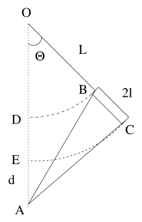
Figure 1: Pendulum with the mass being replaced by a bar magnet. The detecting coil is at ’A’.

where

$$OC = L_{s}+2l$$

$$OB = L_{s}$$

$$OA = L_{s}+2l+d$$

hence,

$$BA^{2} = L_{s}^{2}+(L_{s}+2l+d)^{2}-L_{s}.(L_{s}+2l+d)cos\Theta$$

$$AC^{2} = (L_{s}+2l)^{2}+(L_{s}+2l+d)^{2}-(L_{s}+2l).(L_{s}+2l+d)cos\Theta$$

Based on the assumption that 2l and d are relatively small compared to ${\rm L_{s}}$, the higher powers of 2l and d can be neglected. Hence, eqn(2) can be written as

$$B \approx {\mu_{o}M\over 4\pi}\left[{2l\over L_{s}^{2}(L_{s}+4l+d)(2-cos\Theta)}\right]$$

The induced emf is proportional to the rate of change in the number of magnetic lines cutting the coil.

$${dB\over dt}\approx-{\mu_{o}M\over 4\pi}\left[{2l\over L_{s}^{2}(L_{s}+4l+d)}\right]\left[{sin\Theta\over(2-cos\Theta)^{2}}\right]{d\Theta\over dt}$$

Based on this, the respective induced emf can be written as

$$\xi=-N{dB\over dt}\approx{\mu_{o}MN\over 4\pi}\left[{2l\over L_{s}^{2}(L_{s}+4l+d)}\right]\left[{sin\Theta\over(2-cos\Theta)^{2}}\right]{d\Theta\over dt}$$ (3)

where N is the number of turnings in the coil. Eqn(3) can be written in a compact form

$$\xi=\xi_{o}\left[{sin\Theta\over(2-cos\Theta)^{2}}\right]\left({d\Theta\over dt}\right)$$ (4)

where

$$\xi_{o}={\mu_{o}MN\over 4\pi}\left[{2l\over L_{s}^{2}(L_{s}+4l+d)}\right]$$ (5)

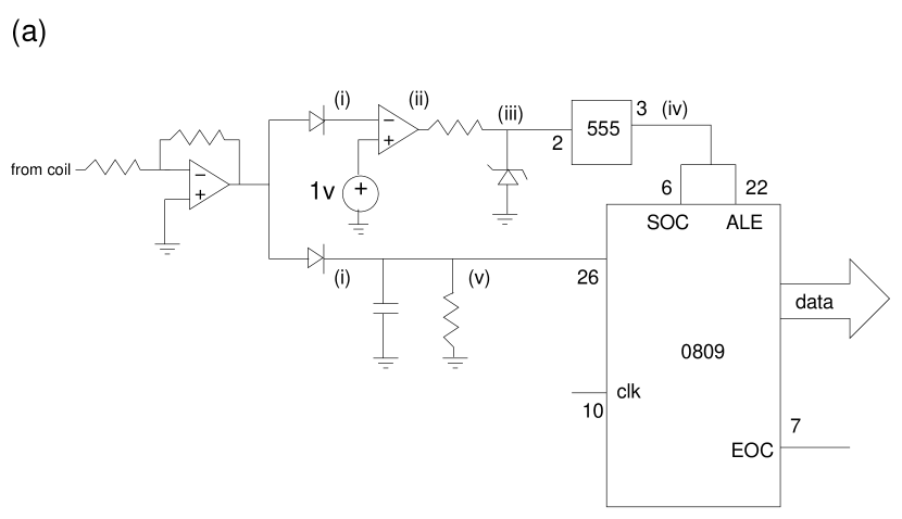
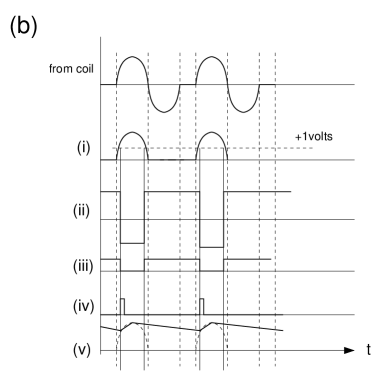
Figure 2: The (a) schematic diagram of the circuit used and the (b) important waveforms at the points marked in the circuit.

Thus, as the distance between the magnet and detecting coil is increased, the induced emf decreases. Infact the induced emf is quite weak and is amplified by an op amp circuit. The high input impedance of the IC741 opamp ensures that a true measurement of the emf is made. To digitalise this analog signal (see fig 1, ref 6) using an Analog to Digital Convertor ADC-0809 (see fig 2a), the amplified output is rectified and the peak value is held by charging a capacitor. The capacitor is discharged via a large resistance so that it retains the peak value till the next peak value arrives.

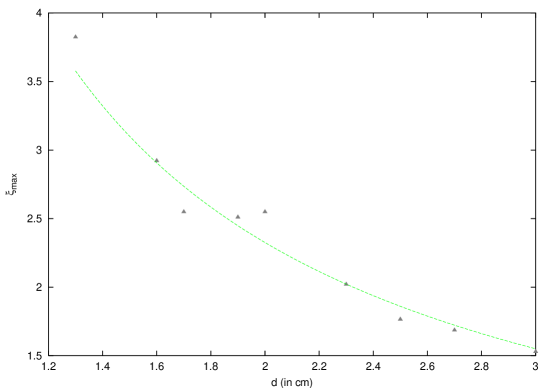
Figure 3: Variation in the maximum induced emf with increasing distance between the coil and the magnet.

We require the ADC to start conversion once the peak value is attained by the capacitor. This implies a synchronization between the input emf pulses and the ADC’s start of conversion (SOC) pulses. To achieve this synchronization it is best to generate the required SOC pulse by wave-shaping the input itself. The amplified input after rectification is fed to a comparator which compares to +1v. This is to avoid spurious/accidental triggering due to noise. The infinite gain results in pulses with sharp edges. The width of these pulses are approximately ${\rm T_{o}/4}$ (for our pendula ${\rm\approx 390ms}$). This would be too large for serving as a SOC and hence is reduced to a ${\rm 5\mu s}$ pulse using a monostable timer made with IC555r8 . The sequencing and synchronization can be understood from the various waveforms shown in fig 2b. The designed circuit digitalises the analog emf and on completion sends an EOC to the computer or microprocessor kit (in case of a microprocessor this is done through a programmable I/O IC8155 chip, details of which can be found in the book by Goankarr7 ) which then reads the eight bit data and stores it for retrivial. This project was done using an 8085 microprocessor kit. The programme and flowchart used is detailed in the Appendix.

The reliability of our circuit can be tested by measuring the maximum emf induced in the coil for varying distances ’d’. Eq(4) shows that the measured maximum emf would be directly proportional to ${\rm\xi_{o}}$ which inturn is inversely proportional to ’d’ (see eqn 5). Fig 3 shows the variation in the experimentally determined ${\rm\xi_{max}}$ with ’d’. While the inverse nature is evident, the value of ${(L_{s}+4l)}$ as returned by curve fitting eqn(5) on our data is substantially off mark from the actual lengths. This is expected since eqn(4) and (5) are very simplified approximations.

III Variation of Induced Emf with Initial Displacement

III.1 While undergoing undamped oscillation

The velocity of an undamped pendulum undergoing SHM is given as

$$\left({d\Theta\over dt}\right)=\omega_{o}\sqrt{\Theta_{m}^{2}-\Theta^{2}}$$

where ${\rm\omega_{o}=\sqrt{g/(L_{s}+2l)}}$ is the frequency of oscillation and ${\rm\Theta_{m}}$ is the initial displacement given to the pendulum. Therefore, the emf induced by our pendulum undergoing undamped SHM would be given as (using eq 4)

$$\xi\approx\omega_{o}\xi_{o}\left[{sin\Theta\sqrt{\Theta_{m}^{2}-\Theta^{2}}\over(2-cos\Theta)^{2}}\right]$$ (6)

The variation in induced emf with time of an undamped pendulum undergoing SHM is as calculated using eqn(6) is shown in fig(4). The maximum angular displacement used to generate the graph using eqn(6) was ${\rm 5^{o}}$. The emf pulse shown in fig 4 is only for half a cycle starting from one extreme position to the opposite extreme. As the magnet approaches the coil, the flux increases and as it crosses the mean position, the emf is negative since the magnet is receding from the coil. Eventhough the velocity (${\rm d\Theta/dt}$) is maximum at the mean position, since the variation in flux (${\rm d\phi/dt}$) is zero, the induced emf is zero as the pendulum passes the mean position.

Figure 4: A measure of the induced emf with oscillating angle. The graph was generated using eqn(6) with ${\rm\Theta_{m}=5^{o}}$.

The position of the pendulum when the maximum emf is generated (between ${\rm 0<\Theta<\Theta_{m}}$) can be found as a problem of maxima and minima

$${d\xi\over d\Theta} = \xi_{o}\left\{{(2-cos\Theta)^{2}\left[sin\Theta{d\over d\Theta}\left({d\Theta\over dt}\right)+cos\Theta\left({d\Theta\over dt}\right)\right]-(2-cos\Theta)sin^{2}\Theta\left({d\Theta\over dt}\right)\over(2-cos\Theta)^{3}}\right\}$$

$$= \xi_{o}\left\{{(2-cos\Theta)\left[sin\Theta{d\over d\Theta}\left({d\Theta\over dt}\right)+cos\Theta\left({d\Theta\over dt}\right)\right]-sin^{2}\Theta\left({d\Theta\over dt}\right)\over(2-cos\Theta)^{2}}\right\}$$

For cases of small angle oscillations eqn(LABEL:eq11) reduces to

$${d\xi\over d\Theta} = \xi_{o}\left[\Theta{d\over d\Theta}\left({d\Theta\over dt}\right)+(1-\Theta^{2})\left({d\Theta\over dt}\right)\right]$$ (7)

$${d\xi\over d\Theta}=\omega_{o}\xi_{o}\left[{-2\Theta^{2}\over 2\sqrt{\Theta_{m}^{2}-\Theta^{2}}}+(1-\Theta^{2})\sqrt{\Theta_{m}^{2}-\Theta^{2}}\right]$$

$$\Theta^{2}=(1-\Theta^{2})(\Theta_{m}^{2}-\Theta^{2})$$

Solving the quadratic equation

$$\Theta^{4}-(2+\Theta_{m}^{2})\Theta^{2}+\Theta_{m}^{2}=0$$

we have

$$\Theta_{peak}=\pm{\Theta_{m}\over\sqrt{2}}$$ (8)

Since eqn(7) was used to determine position of extrema, the above condition is only valid for undamped small angle oscillations. The maxima as per this condition for magnet oscillating through ${\rm\Theta_{m}=5^{o}}$ occurs at ${\rm\pm 0.0617}$ radians (or ${\rm\pm 3.53^{o}}$). The maximum emf that is induced, hence is (use eqn 6)

$$\xi_{max}=\omega_{o}\xi_{o}{\Theta_{m}\over\sqrt{2}}\times{sin{\Theta_{m}\over\sqrt{2}}\over\left(2-cos{\Theta_{m}\over\sqrt{2}}\right)^{2}}$$

Since, these equations and conditions are essentially valid for small angles,

$$\xi_{max}=\left({\omega_{o}\xi_{o}\over 2}\right)\Theta_{m}^{2}$$ (9)

However, a physical pendulum is prone to damping and hence in the next section we investigate as to how the maximum induced emf varies with initial displacement for a damped pendulum.

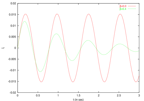
Figure 5: Variation of induced emf when oscillation is damped (${\rm\beta=0.45s^{-1}}$) is compared with the case of no damping (i.e. ${\rm\beta=0.0s^{-1}}$).

III.2 While undergoing damped oscillation

Figure 6: The variation of induced emf of fig 3 is plotted w.r.t. angular position of the pendulum (i.e. ${\rm\Theta}$) for the cases (a) ${\rm\beta=0.0s^{-1}}$ and (b) ${\rm\beta=0.45s^{-1}}$.

We have already stated in our introduction that the damped motion described by eqn(1) exhibits how the pendulum’s oscillation amplitude decreases exponentially with time. The EOM whose solution is given by eqn(1) describes a linear system. The solution can be further trivialized without losing any generality as

$$\Theta=\Theta_{m}e^{-\beta t}sin(\omega^{\prime}t)$$ (10)

from which the velocity can be calculated as

$${d\Theta\over dt} = \omega^{\prime}\Theta_{m}e^{-\beta t}cos(\omega^{\prime}t)-\beta\Theta_{m}e^{-\beta t}sin(\omega^{\prime}t)$$ (11)

$$= \Theta_{m}e^{-\beta t}[\omega^{\prime}cos(\omega^{\prime}t)-\beta sin(\omega^{\prime}t)]$$

Substituting the above expression in eqn(4) we obtain the relation showing the variation of induced emf with time. This variation is shown in fig 5. It is also clear from the figure that the peaks in the induced emf occurs at ${\rm\omega t=(2n+1){\pi\over 4}}$. Hence, the angles at which maxima occur in general is written as

$$\Theta_{peak}=\pm{\Theta_{m}\over\sqrt{2}}e^{-{(2n+1)\pi\over 4tan\phi}}$$ (12)

where ${\rm tan\phi=\omega^{\prime}/\beta}$. Our circuit is designed only to measure peak emfs at n=0,2,4,6….., where only the positive solutions of eqn(12) would contribute. Using our condition on eqn(11) and eqn(4) we have

$$\left({d\Theta\over dt}\right)_{peak}=(\omega^{\prime}-\beta){\Theta_{m}\over\sqrt{2}}e^{-{(2n+1)\pi\over 4tan\phi}}$$

$$\xi_{peak}=(\omega^{\prime}-\beta)\xi_{o}\left[{sin{\Theta_{m}\over\sqrt{2}}e^{-{(2n+1)\pi\over 4tan\phi}}\over(2-cos{\Theta_{m}\over\sqrt{2}}e^{-{(2n+1)\pi\over 4tan\phi}})^{2}}\right]{\Theta_{m}\over\sqrt{2}}e^{-{(2n+1)\pi\over 4tan\phi}}$$ (13)

For small angle oscillations eqn(13) reduces to

$$\xi_{peak}={(\omega^{\prime}-\beta)\xi_{o}\over 2}\Theta_{m}^{2}e^{-{(2n+1)\pi\over 2tan\phi}}$$ (14)

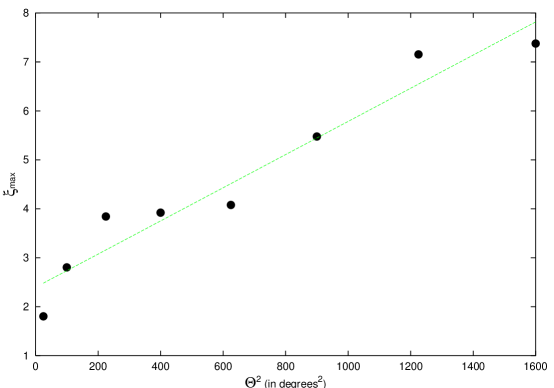
Figure 7: The variation of induced emf with the initial angular displacement of the pendulum. It shows the expected parabolic dependence (i.e. ${\rm\Theta^{2}_{m}}$).

The variation in emf (seen w.r.t time in fig 5) when viewed w.r.t oscillating angle ${\rm\Theta}$ shows how the peak position decreases (eq 12) as also the amplitude of the maximum induced emf decreases (eqn 14) with each half cycle. Eqn(9) and eqn(14) shows that the maximum emf induced for damped pendulums undergoing SHM is directly proportional to the square of maximum angular displacement given to the pendulum. We have recorded the first maxima reading (i.e. n=0) of the induced emf for various angles upto ${\rm 40^{o}}$. The linear relation between ${\rm\xi_{max}}$ and ${\rm\Theta_{m}^{2}}$ is evident. Before commenting further, it must be recollected that eq(1) is valid for small angle oscillations, i.e. for ${\rm\Theta_{m}<5^{o}}$, yet a good linearity is obtained till ${\rm\Theta=40^{o}}$.

Experimental data for ${\rm\Theta_{m}\geq 45^{o}}$ deviate markedly from this linear trend. Remember eqn(12) was obtained with the assumption that the pendula’s motion is described by eqn(10). This equation describes the motion of a pendulum oscillating in a viscous medium with small velocity. It would be shown in the next section that the pendulum’s velocity is quite appreciable for ${\rm\Theta_{m}\geq 45^{o}}$ and hence it’s motion is not described as in eqn(10), explaining the departure for linearity.

IV Results and Observations

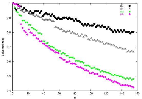
Figure 8: The variation in peak induced emf measured with each oscillation is shown for initial displacements (${\rm\Theta_{m}}$) (a) $\rm 5^{o}$, (b) $\rm 30^{o}$, (c) $\rm 55^{o}$ and (d) $\rm 65^{o}$.

Our prelimary measurements are in good correspondence with commonly known notions and hence we proceed to investigate further the nature of damping in our pendula. It should be noted that the amount of damping and it’s nature are strongly pendula dependent and all results reported here are specific to our experiment and can not be taken as general. We have recorded the maxima in induced emfs for 80 oscillations for various initial displacements. Since for each oscillations, we get two positive maxima in induced emf, figure 8 shows the variation in maxima reading of induced emf for 160 peaks.

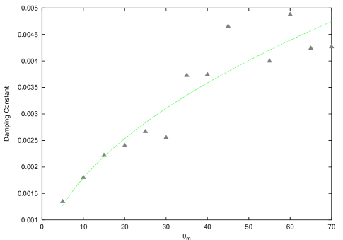
Figure 9: The variation decay constant (b of general equation ${\rm ae^{-bn}}$) of the exponentially decaying region. The continuous line is the parabolic fit for the data points (${\rm 0.00056\sqrt{\Theta_{m}}}$).

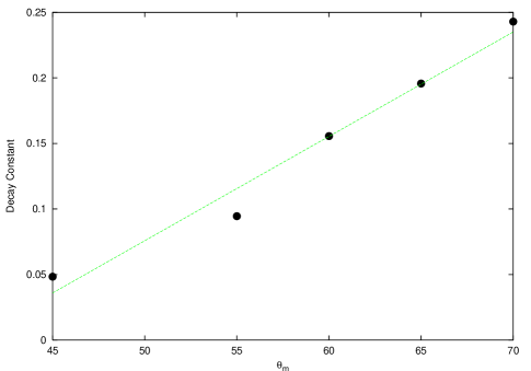
Figure 10: The variation decay in ’b’, a measure of decay in the early oscillations when pendulum was set in motion with displacements ${\rm>45^{o}}$.

A general expression ${\rm ae^{-bn}}$ was fitted to the data of ${\rm\xi_{max}}$ w.r.t n using a standard and freely available curve fitting software called ”Curxpt v3.0”. Good fits were obtained for oscillations set by initial displacements upto ${\rm 40^{o}}$. The exponential fall in emf is indicative of the rate of loss of energy from the oscillating system. It indicates the loss to follow the relation

$${dE\over dt}\propto-E$$

or

$${dE\over dt}=-bE$$

This indicates that the velocity is low and hence the damping/resistive force acting on the pendulum is proportional to the velocityr9 . Figure 9 shows the variation of the decay constant ’b’ (of ${\rm ae^{-bn}}$) with respect to the maximum displacement (${\rm\Theta_{m}}$) given to the pendulum. The graph indicates that as ${\rm\Theta_{m}}$ increases, the velocity with which the pendulum moves increases with which the damping constant increases.

For displacement angles beyond ${\rm 45^{o}}$ (${\rm\Theta_{m}\geq 45^{o}}$), eventhough visual examination of the curves in fig 8 suggests an exponential damping, the data points do not fit to an exponential fall relation. A detailed examination suggests a more complex process is taking place with initial damping being sharper. Infact the initial 25-30 data points fit to ${\rm a/n^{b}}$. The data beyond this fit to the exponential fall equation. The ${\rm a/n^{b}}$ fit corresponds to the damping force being proportional to higher powers of velocity (${\rm v^{\gamma}}$, where ${\rm\gamma>1}$) and in turn the rate of energy loss also being proportional to higher terms of energy. That is, the rate of energy loss for our pendulum set into oscillations with a displacement angle ${\rm>45^{o}}$ is given as

$${dE\over dt}=-\alpha E^{1+b\over b}$$

Figure 10 plots ’b’ versus ${\rm\Theta_{m}}$. The power term (b) is being treated as a measure of damping and is consistent with the results of fig 9, i.e. as initial displacement increases the damping becomes large with a proportionality to the pendulum’s velocity.

The resistive force being proportional to higher powers of velcoity has been reported earlier alsor3 ; r4 ; r13 ; r14 ; r15 ; r16 . A system is reported to have a constant friction (${\rm\gamma=0}$) or a linear dependence of velocity (${\rm\gamma=1}$) or a quadratic depenence of velocity (${\rm\gamma=2}$). Corresponding to which the pendulum’s amplitude decays linearly, exponentially and inverse power decay respectively with time. It hence maybe concluded that for our pendulum sent into motion by initial displacements ${\rm\Theta\geq 45^{o}}$, the damping force is proportional to ${\rm v^{\gamma}}$ where ${\rm\gamma>1}$.

V Conclusion

A simple experiment of setting a suspended bar magnet into oscillations, is a rich source of information. Not only does it give exposure to Faraday’s induction law and a basic understanding of induced emf’s dependence on angle of oscillation, it enables us to study the damping effects on the pendulum. This method is better than previously used methods since the measuring technique does not introduce additional contributions to damping. When the oscillation imparted to the pendulum is very large, the damping effect is also strong with the damping force being proportional to ${\rm v^{\gamma}}$, where ${\rm\gamma>1}$ and ’v’ is the pendulum’s velocity. This brings down the oscillation amplitude of the pendulum and it’s velocity. As the velocity becomes low, the resistive force acting on the pendulum changes it’s nature and becomes proportional to ’v’. Considering the rich information obtained from the experiment and the simplicity of the experiment, it allows the method to be easily implemented as a routine experiment in undergraduate laboratories.

Appendix

Table 1. Program used to collect data.

Address	Mnemonics	Hex Code	Address	Mnemonics	Hex Code
C400	LXI SP	31	C40A	01H	01
C401	00H	00	C40B	JZ	CA
C402	C3H	C3	C40C	07H	07
C403	MVI A	3E	C40D	C4H	C4
C404	00H	00	C40E	IN	DB
C405	OUT	D3	C40F	09H	09
C406	08H	08	C410	PUSH PSW	F5
C407	IN	DB	C411	JMP	C3
C408	OBH	OB	C412	07H	07
C409	ANI	E6	C413	C4H	C4

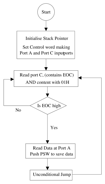
Figure 11: Flowchart.

References

- (1) Gregory M. Quist, ”The PET and pendulum: An application of microcomputers to undergraduate laboratory”, Am. J. Phys., 51, 145-148 (1983).
- (2) M. F. Mclnerney, ”Computer-aided experiments with the damped harmonic oscillator”, Am. J. Phys., 53, 991-996 (1985).
- (3) A. R. Ricchiuto and A. Tozzi, ”Motion of a harmonic oscillator with sliding and viscous friction”, Am. J. Phys., 50, 176-179 (1982).
- (4) Patrick T. Squire, ”Pendulum Damping”, Am. J. Phys., 54, 984-991 (1986).
- (5) Neha Agarwal, Nitin Verma and P. Arun, ”Simple Pendulum revisited”, European. J. Phys., 26, 517-523 (2005).
- (6) Avinash Singh, Y. N. Mohapatra and Satyendra Kumar, ”Electromagnetic induction and damping: Quantitative experiments using a PC interface”, Am. J. Phys., 70, 424-427 (2002).
- (7) L.F.C. Zonetti, A.S.S. Camargo, J. Sartori, D.V de Sousa and L.A.O. Nunes, ”A demonstration of dry and viscous damping of an oscillating pendulum”, Eur. J. Phys., 20, 85-88 (1999).
- (8) John C. Simbach and Joseph Priest, ”Another look at a damped physical pendulum”, Am. J. Phys., 73, 1079-1080 (2005).
- (9) Xiao-jun Wang, Chris Schmitt and Marvin Payne, ”Oscillation with three damping effects”, Eur. J. Phys., 23, 155-164 (2002).
- (10) Ramakant A. Gayakwad, ”Opamps and Linear Integrated Circuits”, Prentice-Hall India, Delhi (1999).
- (11) Ramesh S. Gaonkar, ”Microprocessor Architecture, Programming and applications with the 8085/8080A”, Wiley Eastern Ltd. Delhi (1986).
- (12) Avinash Singh, arXiv:physics/0206086.
- (13) B. J. Miller, ”More Realistic Treatment of the Simple Pendulum without Difficult Mathematics”, Am. J. Phys., 42, 298-303 (1974).
- (14) F. S. Crawford, ”Damping of a simple pendulum”, Am. J. Phys. 43, 276-277 (1975).
- (15) N. F. Pederson and O. H. Soerensen, ”The compound pendulum in intermediate laboratories and demonstrations”, Am. J. Phys. 45, 994-998 (1977).
- (16) R. A. Nelson and M. C. Olsson, ”The pendulum: Rich physics from a simple system”, Am. J. Phys. 54, 112-121 (1986).