The application of the modified form of Båth’s law to the North Anatolian Fault Zone

Abstract

Earthquakes and aftershock sequences follow several empirical scaling laws: One of these laws is Båth’s law for the magnitude of the largest aftershock. In this work, Modified Form of Båth’s Law and its application to KOERI data have been studied. Båth’s law states that the differences in magnitudes between mainshocks and their largest detected aftershocks are approximately constant, independent of the magnitudes of mainshocks and it is about $1.2$. In the modified form of Båth’s law for a given mainshock we get the inferred largest aftershock of this mainshock by using an extrapolation of the Gutenberg-Richter frequency-magnitude statistics of the aftershock sequence. To test the applicability of this modified law, $6$ large earthquakes that occurred in Turkey between $1950$ and $2004$ with magnitudes equal to or greater than $6.9$ have been considered. These earthquakes take place on the North Anatolian Fault Zone. Additionally, in this study the partitioning of energy during a mainshock-aftershock sequence was also calculated in two different ways. It is shown that most of the energy is released in the mainshock. The constancy of the differences in magnitudes between mainshocks and their largest aftershocks is an indication of scale-invariant behavior of aftershock sequences.

1 INTRODUCTION

An earthquake is a sudden and sometimes catastrophic movement of a part of the Earth’s surface [1]. It is caused by the release of stress accumulated along geologic faults or by volcanic activity, hence the earthquakes are the Earth’s natural means of releasing stress. When the Earth’s plates move against each other, stress is put on the lithosphere. When this stress is strong enough, the lithosphere breaks or shifts. As the plates move they put forces on themselves and each other. When the force is large enough, the crust is forced to break. When the break occurs, the stress is released as energy which moves through the Earth in the form of waves, which we feel and call an earthquake.

Aftershocks are earthquakes in the same region of the mainshock[1]. Smaller earthquakes often occur in the immediate area of the main earthquake until the entire surface has reached equilibrium of stress. There are several scaling laws that describe the statistical properties of aftershock sequences [2, 3, 4]. Gutenberg-Richter frequency-magnitude scaling law is widely known by seismologists and scientists. On the Richter scale, the magnitude (M) of an earthquake is proportional to the log of the maximum amplitude of the earth’s motion. What this means is that if the Earth moves one millimeter in a magnitude $2.0$ earthquake, it will move ten millimeters in a magnitude $3.0$ earthquake, $100$ millimeters in a magnitude $4.0$ earthquake and ten meters in a magnitude $6.0$ earthquake. So, the amplitude of the waves increases by powers of ten in relation to the Richter magnitude numbers. Therefore, if we hear about a magnitude $8.0$ earthquake and a magnitude $4$ earthquake, we know that the ground is moving $10,000$ times more in the magnitude $8.0$ earthquake than in the magnitude $4.0$ earthquake. Numbers for the Richter scale range from $0$ to $9.0$, though no real upper limit exists. The difference in energies is even greater. For each factor of ten in amplitude, the energy grows by a factor of $32$. When seismologists started measuring the magnitudes of earthquakes, they found that there were a lot more small earthquakes than large ones. Seismologists have found that the number of earthquakes is proportional to $10^{-bM}$. They call this law “The Gutenberg-Richter Law” [3, 4, 5].

In seismological studies, the Omori law, proposed by Omori in $1894$, is one of the few basic empirical laws [6]. This law describes the decay of aftershock activity with time. Omori Law and its modified forms have been used widely as a fundamental tool for studying aftershocks [7]. Omori published his work on the aftershocks of earthquakes, in which he stated that aftershock frequency decreases by roughly the reciprocal of time after the main shock. An extension of the modified Omori’s law is the epidemic type of aftershock sequences (ETAS) model [7]. It is a stochastic version of the modified Omori law. In the ETAS model, the rate of aftershock occurrence is an effect of combined rates of all secondary aftershock subsequences produced by each aftershock [8, 9].

The third scaling law relating the aftershocks is Båth’s law. The empirical Båth’s law states that the difference in magnitude between a mainshock and its largest aftershock is constant, regardless of the mainshock magnitude and it is about $1.2$ [3, 4, 7, 10]. That is

$$\Delta m=m_{ms}-m_{as}^{max}$$ (1)

with $m_{ms}$ the magnitude of the mainshock, $m_{as}^{max}$ the magnitude of the largest detected aftershock, and $\Delta m$ approximately a constant.

In this article we study the modified form of Båth’s law [3, 4]. To study the aftershock sequence in the North Anatolian Fault Zone (NAFZ) we get the largest aftershock from an extrapolation of the G-R frequency-magnitude scaling of all measured aftershocks. We test the applicability of Båth’s law for $6$ large earthquakes on the North Anatolian Fault Zone (NAFZ). The emprical form of Båth’s law states that the difference magnitude between a mainshock and its largest aftershock is constant, independent of the magnitudes of mainshocks. We also analyze the partitioning of energy during a mainshock-aftershock sequence and its relation to the modified Båth’s law.

2 BÅTH’S LAW AND ITS MODIFIED FORM

Båth’s law states that the differences in magnitudes between mainshocks and their largest aftershocks are approximately constant, independent of the magnitudes of mainshocks. In modified form of Båth’s law for a given mainshock we get the inferred largest aftershock of this mainshock by using an extrapolation of the Gutenberg-Richter frequency-magnitude statistics of the aftershock sequence. The size distribution of earthquakes has been found to show a power law behavior. Gutenberg and Richter, introduced the common description of the frequency of earthquakes: [5]

$$log_{10}N(\geq m)=a-bm$$ (2)

where $N(\geq m)$ is the cumulative number of earthquakes with magnitudes greater than m occurring in a specified area and time window. On this equation a and b are constants. This relation is valid for earthquakes with magnitudes above some lower cutoff $m_{c}$. Earlier studies [3, 4, 11] gave an estimate for this “b” value between $0.8$ and $1.2$. The constant “a” shows the regional level of seismicity and gives the logarithm of the number of earthquakes with magnitudes greater than zero [3, 4]. In our analysis a-value is in the range $3.8<a<6.5$. Aftershocks related with a mainshock also satisfy G-R scaling (2) to a good approximation [3]. In this case $N(\geq m)$ is the cumulative number of aftershocks of a given mainshock with magnitudes greater than m. We offer to extrapolate G-R scaling (2) for aftershocks. Our aim is to obtain an upper cutoff magnitude in a given aftershock sequence. We find the magnitude of this inferred “largest” aftershock $m^{*}$ by formally taking $N(\geq m^{*})=1$ for a given aftershock sequence.

$$a=bm^{*}$$ (3)

This extrapolated $m^{*}$ value will have a mean value and a standard deviation from the mean value. We apply the Båth’s law to the inferred values of $m^{*}$ and then, we can write

$$\Delta m^{*}=m_{ms}-m^{*}$$ (4)

where $m_{ms}$ is the magnitude of the mainshock and $\Delta m^{*}$ is approximately a constant. Substitution of equations (3) and (4) into equation (2) gives

$$log_{10}[N(\geq m)]=b(m_{ms}-\Delta m^{*}-m)$$ (5)

with b, $m_{ms}$, and $\Delta m^{*}$ specified, the frequency-magnitude distribution of aftershocks can be determined using equation (5). In extrapolating the G-R scaling (2) the slope of this scaling or b-value plays an important role in estimating the largest inferred magnitude $m^{*}$.

3 APPLICATION OF THE MODIFIED FORM OF BÅTH’S LAW TO THE NORTH ANATOLIAN FAULT ZONE (NAFZ)

We applied modified form of Båth’s law by considering $6$ large earthquakes on the NAFZ. These earthquakes occurred between $1950$ and $2004$. The data were provided by Bogazici University Kandilli Observatory and Earthquake Research Institute (KOERI)[12]. The $6$ earthquakes considered had magnitudes $m_{ms}\geq 6.9$. The important point is that they were sufficiently separated in space and time so that no aftershock sequences overlapped with other mainshocks. Earthquakes form a hierarchical structure in space and time. Therefore, in some cases it is possible to discriminate foreshocks, mainshocks, and aftershocks. But, generally this classification is not well defined and can be ambiguous. One of our main problems in the study of aftershocks is to identify what is and what is not an aftershock [13]. To specify aftershocks we defined space and time windows for each sequence. In each case we consider a square area centered on the mainshock epicenter. The linear size of the box is taken to be of the order of the linear extent of the aftershock zone L, which scales with the magnitude of the mainshock as

$$L=0.02\times 10^{0.5m_{ms}}km$$ (6)

This equation was given by Yan Y. Kagan [14]. Previously, Shcherbakov and Turcotte used the same scaling arguments for $10$ earthquakes in California [3, 4]. Time intervals of $92$, $183$, $365$, $730$, and $1095$ days are taken except Çanakkale-Yenice, Muş-Varto, and Adapazarı-Mudurnu earthquakes. It should also be noted that for all $6$ earthquakes we took $m_{L}$, Richter magnitudes.

For Kocaeli-Gölcük earthquake the mainshock is $m_{ms}=7.4$ and the largest detected aftershock had a magnitude $m_{as}^{max}=5.8$. From equation (1) the difference in magnitude between the mainshock and largest aftershock is $\Delta m=1.6$. We have correlated the aftershock frequency magnitude data given in Figure 1 with G-R scaling (2) and find $b=0.91\pm 0.05$ and $a=4.97\pm 0.20$. From equation (3) the inferred magnitude of the largest aftershock is $m^{*}=5.46\pm 0.37$. From equation (4) the difference in magnitude between the mainshock and the inferred largest aftershock is $\Delta m^{*}=1.94\pm 0.37$. We applied the same procedure to the all $6$ earthquakes and found a, b, $m^{*}$, and $\Delta m^{*}$ parameters.

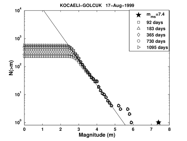
Figure 1: Frequency-magnitude distribution of Kocaeli-Gölcük earthquake

For these $6$ earthquakes, the a, b, $m_{ms}$, $m_{as}^{max}$, $\Delta m$, $m^{*}$, and $\Delta m^{*}$ values are given in Table 1.

Table 1: Summaries of the data and results that show b and a parameters

Earthquake	Date (mm/dd/yy)	b	a
Çanakkale-Yenice	03/18/53	$0.82\pm 0.07$	$4.69\pm 0.33$
Bolu-Abant	05/26/57	$0.61\pm 0.05$	$3.81\pm 0.24$
Muş-Varto	08/19/66	$0.95\pm 0.09$	$5.20\pm 0.37$
Adapazarı-Mudurnu	07/22/67	$1.22\pm 0.10$	$6.62\pm 0.45$
Kocaeli-Gölcük	08/17/99	$0.91\pm 0.05$	$4.97\pm 0.20$
Düzce	11/12/99	$0.80\pm 0.03$	$4.85\pm 0.13$

Table 2: Summaries of the data and results that show $m_{ms}$, $m_{as}^{max}$, $\Delta m$, $m^{*}$, $\Delta m^{*}$ parameters

Earthquake	$m_{ms}$	$m_{as}^{max}$	$\Delta m$	$m^{*}$	$\Delta m^{*}$
Çanakkale-Yenice	7.2	5.4	1.8	$5.72\pm 0.63$	$1.48\pm 0.63$
Bolu-Abant	7.1	5.9	1.2	$6.25\pm 0.65$	$0.85\pm 0.65$
Muş-Varto	6.9	5.3	1.6	$5.47\pm 0.65$	$1.43\pm 0.65$
Adapazarı-Mudurnu	7.2	5.4	1.8	$5.43\pm 0.58$	$1.77\pm 0.58$
Kocaeli-Gölcük	7.4	5.8	1.6	$5.46\pm 0.37$	$1.94\pm 0.37$
Düzce	7.2	5.4	1.8	$6.06\pm 0.28$	$1.14\pm 0.28$

According to our results, the mean of the differences between mainshock and largest detected aftershock magnitudes is $\overline{\Delta m}=1.63\pm 0.23$. The mean of the inferred values of $\Delta m^{*}$ obtained from the best fit of equation (5) is $\overline{\Delta m^{*}}=1.42\pm 0.18$. In addition for these earthquakes the mean of b values is $\overline{b}=0.81\pm 0.02$.

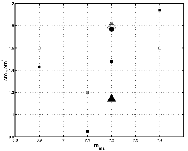
Figure 2: Dispersion of the magnitude differences $\Delta m$ and $\Delta m^{*}$ on the mainshock magnitude $m_{ms}$. White symbols correspond to $\Delta m$ values and black symbols correspond to $\Delta m^{*}$ values.

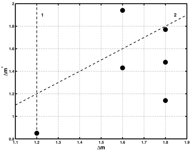
Figure 3: The relation between $\Delta m$ and $\Delta m^{*}$. Line $1$ shows the harmony of our data with the Båth’s Law. Line $2$ corresponds to $y=x$ line and shows the harmony of our data with the Modified Form of Båth’s Law.

4 Radiated Energy During an Earthquake

Seismologists have more recently developed a standard magnitude scale that is called the moment magnitude, and it comes from the seismic moment. To understand the seismic moment, we need to go back to the definition of torque. A torque is an agent that changes the angular momentum of a system. It is defined as the force times the distance from the center of rotation. Earthquakes are caused by internal torques, from the interactions of different blocks of the earth on opposite sides of faults. It can be shown that the moment of an earthquake is simply expressed by

$$M_{0}=\mu Ad$$ (7)

where $M_{0}$=Moment, $\mu$=Rock Rigidity, A=Fault Area, and d=Slip Distance. Both the magnitude and the seismic moment are related to the amount of energy that is radiated by an earthquake. Radiated energy is a particularly important aspect of earthquake behavior, because it causes all the damage and loss of life, and additionally, it is the greatest source of observational data. So, the seismic radiated energy is an important physical parameter to study on earthquakes. The relationships between the radiated energy, stress drop, and earthquake size provides information about the physics of the rupture process. Richter and Gutenberg, developed a relationship between magnitude and energy. Their relationship is:

$$log_{10}[E(m)]=\frac{3}{2}m+11.8$$ (8)

It should be noted that in this relation E(m) is not the total “intrinsic” energy of the earthquake. It is only the radiated energy from the earthquake and a small fraction of the total energy transferred during the earthquake process. We can write this equation in this form [3, 15].

$$log_{10}[E(m)]=\frac{3}{2}m+log_{10}E_{0}$$ (9)

with $E_{0}=6.3\times 10^{4}J$. Our aim is to determine the ratio of the total seismic energy radiated in the aftershock sequence to the seismic energy radiated in the mainshock. This relation can be used directly to relate the radiated energy from the mainshock $E_{ms}$ to the moment magnitude of the mainshock $m_{ms}$

$$E_{ms}=E_{0}10^{(3/2)m_{ms}}$$ (10)

4.1 The First Calculation Method To Find The Energy Ratio Between Mainshock and Aftershock Sequences

The total radiated energy in the aftershock sequence $E_{as}$ is obtained by integrating over the distributions of aftershocks [3]. This can be written

$$E_{as}=\int_{-\infty}^{m_{as}^{max}}E(m)(-\frac{dN}{dm})dm$$ (11)

Taking the derivative of equation (2) with respect to the aftershock magnitude m we have

$$dN=-b(ln10)10^{a-bm}dm$$ (12)

Putting equation (12) into equation (11) gives

$$E_{as}=b(ln10)10^{a}\int_{-\infty}^{m_{as}^{max}}E(m)10^{-bm}dm$$ (13)

In addition, if we turn back to equation (10) and put it to equation (13) we get

$$E_{as}=b(ln10)10^{a}E_{0}\int_{-\infty}^{m_{as}^{max}}10^{(3/2-b)m}dm$$ (14)

Then we take this integral and we find

$$E_{as}=\frac{2b}{(3-2b)}E_{0}10^{a}10^{(3/2-b)m_{as}^{max}}$$ (15)

To find the ratio of the total radiated energy in aftershocks $E_{as}$ to the radiated energy in the mainshock $E_{ms}$, we divide equation (15) to equation (10). Then we get the result

$$\frac{E_{as}}{E_{ms}}=\frac{2b}{(3-2b)}10^{a}10^{-bm_{as}^{max}}10^{-3/2(m_{ms}-m_{as}^{max})}$$ (16)

We know that $\Delta m=m_{ms}-m_{as}^{max}$ so equation (16) takes this form:

$$\frac{E_{as}}{E_{ms}}=\frac{2b}{(3-2b)}10^{a}10^{-bm_{as}^{max}}10^{-3/2(\Delta m)}$$ (17)

From the equation (17), the fraction of the total energy associated with aftershocks is given by

$$\frac{E_{as}}{E_{ms}+E_{as}}=\frac{1}{1+(\frac{3-2b}{2b})10^{3/2\Delta m}10^{-(a-bm_{as}^{max})}}$$ (18)

For the $6$ earthquakes considered in the previous section we had put the b, a, $\Delta m$ and $m_{as}^{max}$ values to equation (18) individually. Our aim is to find $\frac{E_{as}}{E_{ms}+E_{as}}$ values for $6$ earthquakes.

Table 3: Summaries of the data and results for energy values that were taken from the first energy calculation method

Earthquake	a	b	$m_{as}^{max}$	$\Delta m$	$\frac{E_{as}}{E_{ms}+E_{as}}$
Çanakkale-Yenice	$4.69\pm 0.33$	$0.82\pm 0.07$	5.4	1.8	0.004
Bolu-Abant	$3.81\pm 0.24$	$0.61\pm 0.05$	5.9	1.2	0.017
Muş-Varto	$5.20\pm 0.37$	$0.95\pm 0.09$	5.3	1.6	0.010
Adapazarı-Mudurnu	$6.62\pm 0.45$	$1.22\pm 0.10$	5.4	1.8	0.009
Kocaeli-Gölcük	$4.97\pm 0.20$	$0.91\pm 0.05$	5.8	1.6	0.002
Düzce	$4.85\pm 0.13$	$0.80\pm 0.03$	5.4	1.8	0.008

According to our results, we find the mean energy $\frac{E_{as}}{E_{ms}+E_{as}}=0.008$ with a standard deviation $\sigma_{\overline{E}}=0.005$. Consequently, we find that for these earthquakes on average about $99.2$ per cent of the available elastic energy is released during the mainshock and about $0.8$ per cent of energy is released during the aftershocks.

4.2 The Second Calculation Method To Find The Energy Ratio Between Mainshock and Aftershock Sequences

Additionally, from the study of Shcherbakov and Turcotte in $2004$ [3, 4], we may derive the same energy ratio in terms of b and $\Delta m^{*}$ values.

The total radiated energy in the aftershock sequence $E_{as}$ is obtained by integrating over the distributions of aftershocks [3]. This can be written

$$E_{as}=\int_{-\infty}^{m^{*}}E(m)(-\frac{dN}{dm})dm$$ (19)

Taking the derivative of equation (5)with respect to the aftershock magnitude m we have

$$dN=-b(ln10)10^{b(m_{ms}-\Delta m^{*}-m)}dm$$ (20)

Putting equation (20) into equation (19) gives

$$E_{as}=b(ln10)10^{b(m_{ms}-\Delta m^{*})}\int_{-\infty}^{m^{*}}E(m)10^{-bm}dm$$ (21)

In addition, if we turn back to equation (10) and put it to equation (21) we get

$$E_{as}=b(ln10)10^{b(m_{ms}-\Delta m^{*})}E_{0}\int_{-\infty}^{m^{*}}10^{(3/2-b)m}dm$$ (22)

Then we take this integral and we find

$$E_{as}=\frac{2b}{(3-2b)}E_{0}10^{(3/2-b)m^{*}}10^{b(m_{ms}-\Delta m^{*})}$$ (23)

Using equation (4) we find

$$E_{as}=\frac{2b}{(3-2b)}E_{0}10^{3/2(m_{ms}-\Delta m^{*})}$$ (24)

To find the ratio of the total radiated energy in aftershocks $E_{as}$ to the radiated energy in the mainshock $E_{ms}$, we divide equation (24) to equation (10). Then we get the result

$$\frac{E_{as}}{E_{ms}}=\frac{2b}{(3-2b)}10^{-3/2\Delta m^{*}}$$ (25)

If we further assume that all earthquakes have the same seismic efficiency (ratio of radiated energy to the total drop in stored elastic energy), then this ratio is also the ratio of the drop in stored elastic energy due to the aftershocks to the drop in stored elastic energy due to the mainshock. From equation (25) the fraction of the total energy associated with aftershocks is given by

$$\frac{E_{as}}{E_{ms}+E_{as}}=\frac{1}{1+\frac{3-2b}{2b}10^{3/2\Delta m^{*}}}$$ (26)

For the $6$ earthquakes considered in the previous section we had put the b and $m^{*}$ values to equation (26) individually. Our aim is to find $\frac{E_{as}}{E_{ms}+E_{as}}$ values for $6$ earthquakes considered. The obtained results are summarized in Table (4).

Table 4: Summaries of the data and results for energy values that were taken from the second energy calculation method

Earthquake	b	$\Delta m^{*}$	$\frac{E_{as}}{E_{ms}+E_{as}}$
Çanakkale-Yenice	$0.82\pm 0.07$	$1.48\pm 0.63$	0.007
Bolu-Abant	$0.61\pm 0.05$	$0.85\pm 0.65$	0.035
Muş-Varto	$0.95\pm 0.09$	$1.43\pm 0.65$	0.012
Adapazarı-Mudurnu	$1.22\pm 0.10$	$1.77\pm 0.57$	0.010
Kocaeli-Gölcük	$0.91\pm 0.05$	$1.94\pm 0.37$	0.002
Düzce	$0.80\pm 0.03$	$1.14\pm 0.28$	0.022

According to our results, we find the mean energy $\frac{E_{as}}{E_{ms}+E_{as}}=0.015$ with a standard deviation $\sigma_{\overline{E}}=0.012$. Consequently, we find that the ratio of radiated energy in aftershocks to the radiated energy in the mainshock is constant. This is consistent with the generally accepted condition of self-similarity for earthquakes. For these earthquakes on average about $98.5$ per cent of the available elastic energy goes into the mainshock and about $1.5$ per cent into the aftershocks.

5 Discussion

Earthquakes occur in clusters. After one earthquake happens, we usually see others at nearby or identical location. Clustering of earthquakes usually occurs near the location of the mainshock. The stress on the mainshock’s fault changes drastically during the mainshock and that fault produces most of the aftershocks. This causes a change in the regional stress, the size of which decreases rapidly with distance from the mainshock. Sometimes the change in stress caused by the mainshock is great enough to trigger aftershocks on other, nearby faults. It is accepted that aftershocks are caused by stress transfer during an earthquake. When an earthquake occurs there are adjacent regions where the stress is increased. The relaxation of these stresses causes aftershocks [3, 16, 17, 18, 19, 20, 21].

Several scaling laws are also found to be universally valid for aftershocks [2, 3, 4]. These are:

1. Gutenberg-Richter frequency-magnitude scaling

2. The modified Omori’s law for the temporal decay of aftershocks

3. Båth’s law for the magnitude of the largest aftershock

In this work we used both Båth’s law and G-R scaling. Our aim is to find an upper cutoff magnitude $m^{*}$ for a given aftershock sequence. Using relation (3), we get related a and b values in the G-R scaling. Båth’s law states that, to a good approximation, the difference in magnitude between mainshock and its largest aftershock is a constant independent of the mainshock magnitude. A modified form of Båth’s law was proposed by Shcherbakov and Turcotte in $2004$ [3, 4]. They considered $10$ large earthquakes that occurred in California between $1987$ and $2003$ with magnitudes equal to or greater than $m_{ms}\geq 5.5$. According to their theory the mean difference in magnitudes between these mainshocks and their largest detected aftershocks is $1.16\pm 0.46$. This result is consistent with Båth’s Law. They found the mean difference in magnitudes between the mainshocks and their largest inferred aftershocks is $1.11\pm 0.29$. They also calculated the partitioning of energy during a mainshock-aftershock sequence and found that about $96$ per cent of the energy dissipated in a sequence is associated with the mainshock and the rest ($4$ per cent) is due to aftershocks. Their results are given in Table 5. We applied the Modified Form of Båth’s Law to our $6$ large earthquakes that occurred on the North Anatolian Fault Zone (NAFZ) in Turkey. We followed the same calculation process.

Table 5: Comparision the results

Parameters	Turcotte and Shcherbakov	Kurnaz and Yalcin
$\overline{\Delta m}$	$1.16\pm 0.46$	$1.63\pm 0.23$
$\overline{\Delta m^{*}}$	$1.11\pm 0.29$	$1.42\pm 0.18$
$\frac{E_{as}}{E_{ms}+E_{as}}$	$0.038$	$0.015$

According to Table 5, for the North Anatolian Fault Zone (NAFZ), a large fraction of the accumulated energy is released in the mainshock and only a relatively small fraction of the accumulated energy is released in the aftershock sequence. The results of Turcotte and Shcherbakov are for the ten earthquakes in California on the San Andreas Fault Zone. Although SAFZ (in California) and NAFZ (in Turkey) have the same seismic properties, the released energy during the mainshocks in the NAFZ is much greater than the released energy during the mainshocks in the SAFZ.

Figure 7 shows the dispersion of the magnitude differences $\Delta m$ and $\Delta m^{*}$ on the mainshock magnitude $m_{ms}$. In this figure, white symbols correspond to $\Delta m$ values and black symbols correspond to $\Delta m^{*}$ values. Square, circle and triangle were used to prevent the coincides of the data on the figure; because for six earthquakes, three of them have the same mainshock magnitude $m_{ms}=7.2$.

Additionally, Figure 8 gives us the relation between $\Delta m$ and $\Delta m^{*}$. In this figure, line $1$ shows the harmony of our data with the Båth’s Law. According to Figure 8, our data do not show harmony with the Båth’s Law. Båth’s Law states that the difference in magnitude between a mainshock and its largest detected aftershock is constant, regardless of the mainshock magnitude and it is about $1.2$ [3, 4, 7, 10]. But in Figure 8, only one earthquake has $\Delta m$ values equal to $1.2$. The other five earthquakes have $\Delta m$ values greater than $1.2$. Consequently, only $17$ per cent of our data show harmony with the Båth’s Law. The rest part ( $83$ per cent) of our data do not show harmony with the Båth’s Law.

The constancy of the differences in magnitudes between mainshocks and their largest aftershocks is an indication of scale-invariant behavior of aftershock sequences.

In Figure 8, line $2$ shows the harmony of our data with the Modified Form of Båth’s Law. This line corresponds to $y=x$ line. If the Modified Form of Båth’s Law gave us perfect results, $\Delta m$ and $\Delta m^{*}$ values would be close to each other along this line. Hence, they would be the near of line $2$. But in Figure 8, only one earthquake takes place on the upper side of this line. The remaining five earthquakes take place on the lower side of this line. Consequently, our data do not show harmony with the Modified Form of Båth’s Law.

The other important conclusion is that we know most of the energy is released during the mainshock. Therefore, after the mainshock the community and government may begin their work to rescue people from the debris without wasting any time.

References

References

- [1] H. Kanamori, Emily E. Brodsky, Reports on Progress in Physics 67, pp1429-1496 (2004).
- [2] C. Kisslinger, Advances in Geophysics 38, pp1-36 (1996).
- [3] R. Shcherbakov, Donald L. Turcotte, Bulletin of the Seismological Society of America 94, pp1968-1975 (2004).
- [4] R. Shcherbakov, Donald L. Turcotte, John B. Rundle, Pure and Applied Geophysics 162, pp1051-1076 (2005).
- [5] B. Gutenberg, C. F. Richter Seismicity of the Earth and Associated Phenomena (Princeton Univ. Press, Princeton, New Jersey, 1954).
- [6] F. Omori, Journal of College of Science of the Imperial University of Tokyo 7, 111-200 (1894).
- [7] A. Helmstetter, D. Sornette, Geophysical Research Letters 30, 10.1029/2003GL018186 (2003).
- [8] Y. Y. Kagan, L. Knopoff, Journal of Geophysical Research 86, 2853-2862 (1981).
- [9] Y. Ogata, Journal of the American Statistical Association 83, 9-27 (1988).
- [10] M. Bath, Tectonophysics 2, 483-514 (1965).
- [11] C. Frolich, S. D. Davis, Journal of Geophysical Research 98, 631-644 (1993).
- [12] Bogazici University Kandilli Observatory and Earthquake Research Institute, http://www.koeri.boun.edu.tr, 2006.
- [13] G. M. Molchan, O. E. Dmitrieva, Geophysical Journal International 109, 501-516 (1992).
- [14] Y. Y. Kagan, Bulletin of Seismological Society of America 92, 641-655 (2002).
- [15] T. Utsu, Relationship between magnitude scales (International Handbook of Earthquake and Engineering Seismology, W. H. K., 2002).
- [16] K. Rybicki, Physics of the Earth and Planetary Interiors 7, 409-422 (1973).
- [17] S. Das, C. H. Scholz, Bulletin of Seismological Society of America 71, 1669-1675 (1981).
- [18] C. Mendoza, S. H. Hartzell, Bulletin of Seismological Society of America 78, 1438-1449 (1988).
- [19] G. C. P. King, R. S. Stein, J. Lin, Bulletin of Seismological Society of America 84, 935-953 (1994).
- [20] A. Marcellini, Journal of Geophysical Research 100, 6463-6468 (1995).
- [21] J. L. Hardebeck, J. J. Nazareth, E. Hauksson, Journal of Geophysical Research 103, 24,427-24,437 (1998).