Growing distributed networks with arbitrary degree distributions

Abstract

We consider distributed networks, such as peer-to-peer networks, whose structure can be manipulated by adjusting the rules by which vertices enter and leave the network. We focus in particular on degree distributions and show that, with some mild constraints, it is possible by a suitable choice of rules to arrange for the network to have any degree distribution we desire. We also describe a mechanism based on biased random walks by which appropriate rules could be implemented in practice. As an example application, we describe and simulate the construction of a peer-to-peer network optimized to minimize search times and bandwidth requirements.

I Introduction

Complex networks, such as the Internet, the worldwide web, and social and biological networks, have attracted a remarkable amount of attention from the physics community in recent years Newman03d ; Boccaletti06 ; DM03b ; NBW06 . Most studies of these systems have concentrated on determining their structure or the effects that structure has on the behavior of the system. For instance, a considerable amount of effort has been devoted to studies of the degree distributions of networks, their measurement and the formulation of theories to explain how they come to take the observed forms, and models of the effect of particular degree distributions on dynamical processes on networks, network resilience, percolation properties, and many other phenomena. Such studies are appropriate for “naturally occurring” networks, whose structure grows or is created according to some set of rules not under our direct control. The Internet, the web, and social networks fall into this category even though they are man-made, since their growth is distributed and not under the control of any single authority.

Not all networks fall in this class however. There are some networks whose structure is centrally controlled, such as telephone networks, some transportation networks, or distribution networks like power grids. For these networks it is interesting to ask how, if one can design the network to have any structure one pleases, one could choose that structure to optimize some desired property of the network. For instance, Paul et al. PTHS04 have considered how the structure of a network should be chosen to optimize the network’s robustness to deletion of its vertices.

In this paper we study a class of networks that falls between these two types. There are some networks that grow in a collaborative, distributed fashion, so that we cannot control the network’s structure directly. But we can control some of the rules by which the network forms and this in turn allows us a limited degree of influence over the structure. The archetypal example of such a system is a distributed database such as a peer-to-peer filesharing network, which is a virtual network of linked computers that share data among themselves. The network is formed by a dynamical process under which individual computers continually join or leave the network, and the rules of joining and leaving can be manipulated to some extent by changing the behavior of the software governing computers’ behaviors. It is well established that the structure of peer-to-peer networks can have a strong effect on their performance ALPH01 ; SBR04 but to a large extent that structure has in the past been regarded as an experimentally determined quantity Hong01 . Here we consider ways in which the structure can be manipulated by changing the behavior of individual nodes so as to optimize network performance.

II Growing networks with desired properties

In this paper we focus primarily on creating networks with desired degree distributions: the degree distribution typically has a strong effect on the behavior of the network and is relatively straightforward to treat mathematically. There are two basic problems we need to address if we want to create a network with a specific degree distribution solely by manipulating the rules by which vertices enter and leave the network. First, we need to find rules that will achieve the desired result, and second, we need to find a practical mechanism that implements those rules and operates in reasonable time. We deal with these questions in order.

Our approach to growing a network with a desired degree distribution is based on the idea of the “attachment kernel” introduced by Krapivsky and Redner KR01 . We assume that vertices join our network at intervals and that when they do so they form connections—edges—to some number of other vertices in the network. By designing the software appropriately, we can in a peer-to-peer network choose the number of edges a newly joining vertex makes and also, as we will shortly show, some crucial aspects of which other vertices those edges connect to.

Let us define $p_{k}$ to be the degree distribution of our network at some time, i.e., the fraction of vertices having degree $k$, which satisfies the normalization condition

$$\sum_{k=0}^{\infty}p_{k}=1.$$ (1)

And let us define the attachment kernel $\pi_{k}$ to be the probability that an edge from a newly appearing vertex connects to a particular preexisting vertex of degree $k$, divided by the number $n$ of vertices in the network. It is this attachment kernel that we will manipulate to produce a desired degree distribution. The extra factor of $n$ in the definition is not strictly necessary, but it is convenient: since the total number of vertices of degree $k$ is $np_{k}$, it means that the probability of a new edge connecting to any vertex of degree $k$ is just $\pi_{k}p_{k}$, and hence $\pi_{k}$ satisfies the normalization condition

$$\sum_{k=0}^{\infty}\pi_{k}p_{k}=1.$$ (2)

In a peer-to-peer network users may exit the network whenever they want and we as designers have little control over this aspect of the network dynamics. We will assume in the calculations that follow that vertices simply vanish at random. We will also assume that, on the typical time-scales over which people enter and leave the network, the total size $n$ of the network does not change substantially, so that the rates at which vertices enter and leave are roughly equal. For simplicity let us say that exactly one vertex enters the network and one leaves per unit time (although the results presented here are in fact still valid even if only the probabilities per unit time of addition and deletion of vertices are equal and not the rates).

Now let us chose the initial degrees of vertices when they join the network, i.e., the number of connections that they form upon entering, at random from some distribution $r_{k}$. Building on our previous results in MGN06 , we observe that the evolution of the degree distribution of our network can be described by a rate equation as follows. The number of vertices with degree $k$ at a particular time is $np_{k}$. One unit of time later we have added one vertex and taken away one vertex, so that the number with degree $k$ becomes

$$np_{k}^{\prime} =np_{k}+c\pi_{k-1}p_{k-1}-c\pi_{k}p_{k}$$

$$\quad{}+(k+1)p_{k+1}-kp_{k}-p_{k}+r_{k},$$ (3)

with the convention that $p_{-1}=0$, and $c=\sum_{k=0}^{\infty}kr_{k}$, which is the average degree of vertices added to the network. The terms $c\pi_{k-1}p_{k-1}$ and $-c\pi_{k}p_{k}$ in Eq. (II) represent the flow of vertices with degree $k-1$ to $k$ and $k$ to $k+1$, as they gain extra edges with the addition of new vertices. The terms $(k+1)p_{k+1}$ and $-kp_{k}$ represent the flow of vertices with degree $k+1$ and $k$ to $k$ and $k-1$, as they lose edges with the removal of neighboring vertices. The term $-p_{k}$ represents the probability of removal of a vertex of degree $k$ and the term $r_{k}$ represents the addition of a new vertex with degree $k$ to the network.

Assuming $p_{k}$ has an asymptotic form in the limit of large time, that form is given by setting $p_{k}^{\prime}=p_{k}$ thus:

$$c\pi_{k-1}p_{k-1}-c\pi_{k}p_{k}+(k+1)p_{k+1} -kp_{k}$$

$${}-p_{k}+r_{k}=0.$$ (4)

Following previous convention NSW01 , let us define a generating function $G_{0}(z)$ for the degree distribution thus:

$$G_{0}(z)=\sum_{k=0}^{\infty}p_{k}z^{k},$$ (5)

as well as generating functions for the degrees of vertices added and for the attachment kernel thus:

$$F(z) = \sum_{k=0}^{\infty}r_{k}z^{k},$$ (6)

$$H(z) = \sum_{k=0}^{\infty}\pi_{k}p_{k}z^{k}.$$ (7)

Multiplying both sides of (II) by $z^{k}$ and summing over $k$, we then find that the generating functions satisfy the differential equation

$$(1-z){\mathrm{d}G_{0}\over\mathrm{d}z}-G_{0}(z)-c(1-z)H(z)+F(z)=0.$$ (8)

We are interested in creating a network with a given degree distribution, i.e., with a given $G_{0}(z)$. Rearranging (8), we find that the choice of attachment kernel $\pi_{k}$ that achieves this is such that

$$H(z)={1\over c}\biggl{[}{\mathrm{d}G_{0}\over\mathrm{d}z}+{F(z)-G_{0}(z)\over 1-z}\biggr{]}.$$ (9)

Taking the limit $z\to 1$, noting that normalization requires that all the generating functions tend to 1 at $z=1$, and applying L’Hopital’s rule, we find

$$1=\frac{1}{c}\left[\langle k\rangle+\langle k\rangle-c\right],$$ (10)

where we have made use of the fact that the average degree in the network is $\langle k\rangle=G_{0}^{\prime}(1)$ and $c=H^{\prime}(1)$. Rearranging, we then find that $c=\langle k\rangle$. In other words, solutions to Eq. (8) require that the average degree $c$ of vertices added to the network be equal to the average degree of vertices in the network as a whole. Making use of this result, we can write Eq. (9) in the form

$$H(z)=G_{1}(z)+{F(z)-G_{0}(z)\over c(1-z)},$$ (11)

where $G_{1}(z)=G_{0}^{\prime}(z)/G_{0}^{\prime}(1)=\sum_{k}q_{k}z^{k}$ is the generating function for the so-called excess degree distribution

$$q_{k}={(k+1)p_{k+1}\over\langle k\rangle},$$ (12)

which appears in many other network-related calculations—see, for instance, Ref. NSW01 .

Now it is straightforward to derive the desired attachment kernel. Noting that

$${1\over 1-z}=\sum_{k=0}^{\infty}z^{k},$$ (13)

we can simply read off the coefficient of $z^{k}$ on either side of Eq. (11), to give

$$\pi_{k}p_{k}=q_{k}+{1\over c}\sum_{m=0}^{k}(r_{m}-p_{m}),$$ (14)

or equivalently

$$\pi_{k}={1\over cp_{k}}\bigl{[}(k+1)p_{k+1}+P_{k+1}-R_{k+1}\bigr{]},$$ (15)

where $P_{k}$ is the cumulative distribution of vertex degrees and $R_{k}$ is the cumulative distribution of added degrees:

$$P_{k}=\sum_{m=k}^{\infty}p_{m},\qquad R_{k}=\sum_{m=k}^{\infty}r_{m}.$$ (16)

Since we are at liberty to choose both $r_{k}$ and $\pi_{k}$, we have many options for satisfying Eq. (15); given (almost) any choice of the distribution $r_{k}$ of the degrees of added vertices, we can find the corresponding $\pi_{k}$ that will give the desired final degree distribution of the network. One simple choice would be to make the degree distribution of the added vertices the same as the desired degree distribution, so that $R_{k}=P_{k}$. Then

$$\pi_{k}={q_{k}\over p_{k}}={(k+1)p_{k+1}\over cp_{k}}.$$ (17)

In other words, if we have some desired degree distribution $p_{k}$ for our network, one way to achieve it is to add vertices with exactly that degree distribution and then arrange the attachment process so that the degree distribution remains preserved thereafter, even as vertices and edges are added to and removed from the network. Equation (17) tells us the choice of attachment kernel that will achieve this. Equation (17) will work for essentially any choice of degree distribution $p_{k}$, except choices for which $p_{k}=0$ and $p_{k+1}>0$ for some $k$. In the latter case Eq. (17) will diverge for some value(s) of $k$.

II.1 Example: power-law degree distribution

As an example, consider the creation of a network with a power-law degree distribution. Adamic et al. ALPH01 have shown that search processes on peer-to-peer networks with power-law degree distributions are particularly efficient, so there are reasons why one might want to generate such a network.

Let us choose

$$p_{k}=\begin{cases}\enspace Ck^{-\gamma}&\text{for $k\geq 1$,}\\ \enspace p_{0}&\text{for $k=0$,}\end{cases}$$ (18)

where $\gamma$ and $p_{0}$ are constants and the normalizing factor $C$ is given by

$$C={1-p_{0}\over\zeta(\gamma)},$$ (19)

where $\zeta(\gamma)$ is the Riemann zeta-function. Then the mean degree is

$$\langle k\rangle=c=(1-p_{0}){\zeta(\gamma-1)\over\zeta(\gamma)},$$ (20)

and Eq. (17) tells us that the correct choice of attachment kernel in this case is

$$\pi_{k}={1\over 1-p_{0}}\,{\zeta(\gamma)\over\zeta(\gamma-1)}\,{k^{\gamma}\over(k+1)^{\gamma-1}},$$ (21)

for $k\geq 1$ and

$$\pi_{0}={1\over p_{0}\zeta(\gamma-1)}.$$ (22)

It is interesting to note that as $k$ becomes large, this attachment kernel goes as $\pi_{k}\sim k$, the so-called (linear) preferential attachment form in which vertices connect to others in simple proportion to their current degree. In growing networks this form is known to give rise, asymptotically, to a power-law degree distribution. It is important to understand, however, that in the present case the network is not growing and hence, despite the apparent similarity, this is not the same result. Indeed, it is known that for non-growing networks, purely linear preferential attachment does not produce power-law degree distributions SR04b ; CFV04 , but instead generates stretched exponential distributions MGN06 . Thus it is somewhat surprising to observe that one can, nonetheless, create a power-law degree distribution in a non-growing network using an attachment kernel that seems, superficially, quite close to the linear form.

Sarshar and Roychowdhury SR04b showed previously that it is possible to generate a non-growing power-law network by using linear preferential attachment and then compensating for the expected loss of power-law behavior by rewiring the connections of some vertices after their addition to the network. Our results indicate that, although this process will certainly work, it is not necessary: a slight modification to the preferential attachment process will achieve the same goal and frees us from the need to rewire any edges.

Note also that (21) is not the only solution of Eq. (15) that will generate a power-law distribution. If we choose a different (e.g., non-power-law) distribution for the vertices added to the network, we can still generate an overall power-law distribution by choosing the attachment kernel to satisfy Eq. (15). Suppose, for instance, that, rather than adding vertices with a power-law degree distribution, we prefer to give them a Poisson distribution with mean $c$:

$$r_{k}=\mathrm{e}^{-c}\,{c^{k}\over k!}.$$ (23)

In this case $R_{k}=1-\Gamma(k,c)/\Gamma(k)$, where $\Gamma(k)$ is the standard gamma function and $\Gamma(k,c)$ is the incomplete gamma function. Then the power law is correctly generated by the choice

$$\pi_{k} ={1\over 1-p_{0}}\,{\zeta(\gamma)\over\zeta(\gamma-1)}\,k^{\gamma}\biggl{[}(k+1)^{-\gamma+1}+\zeta(\gamma,k+1)$$

$$\qquad-{\zeta(\gamma)\over 1-p_{0}}\biggl{(}1-{\Gamma(k+1,c)\over\Gamma(k+1)}\biggr{)}\biggr{]},$$ (24)

for $k\geq 1$, where $\zeta(\gamma,x)$ is the generalized zeta function $\zeta(\gamma,x)=\sum_{k=0}^{\infty}(k+x)^{-\gamma}$. For $k=0$,

$$\pi_{0}={1\over p_{0}\zeta(\gamma-1)}\biggl{[}1+{\mathrm{e}^{-c}-p_{0}\over 1-p_{0}}\,\zeta(\gamma)\biggr{]}.$$ (25)

III A practical implementation

In theory, we should be able use the ideas of the previous section to grow a network with a desired degree distribution. This does not, however, yet mean we can do so in practice. To make our scheme a practical reality, we still need to devise a realistic way to place edges between vertices with the desired attachment kernel $\pi_{k}$. If each vertex entering the network knew the identities and degrees of all other vertices, this would be easy: we would simply select a degree $k$ at random in proportion to $\pi_{k}p_{k}$, and then attach our new edge to a vertex chosen uniformly at random from those having that degree.

In the real world, however, and particularly in peer-to-peer networks, no vertex “knows” the identity of all others. Typically, computers only know the identities (such as IP addresses) of their immediate network neighbors. To get around this problem, we propose the following scheme, which makes use of biased random walks.

A random walk, in this context, is a succession of steps along edges in our network where at each vertex $i$ we choose to step next to a vertex chosen at random from the set of neighbors of $i$. In the context of a peer-to-peer computer network, for example, such a walk can be implemented by message passing between peers. The “walker” is a message or data packet that is passed from computer to neighboring computer, with each computer making random choices about which neighbor to pass to next.

Starting a walk from any vertex in the network, we can sample vertices by allowing the walk to take some fixed number of steps and then choosing the vertex that it lands upon on its final step. We will consider random walks in which the choice of which step to make at each vertex is deliberately biased to create a desired probability distribution for the sample as follows.

Consider a walk in which a walker at vertex $j$ chooses uniformly at random one of the $k_{j}$ neighbors of that vertex. Let us call this neighbor $i$. Then the walk takes a step to vertex $i$ with some acceptance probability $P_{ij}$. The total probability $T_{ij}$ of a transition from $j$ to $i$ given that we are currently at $j$ is

$$T_{ij}={A_{ij}\over k_{j}}P_{ij},$$ (26)

where $k_{j}$ is the degree of vertex $j$ and $A_{ij}$ is an element of the adjacency matrix:

$$A_{ij}=\begin{cases}\enspace 1&\text{if there is an edge joining vertices $i,j$,}\\ \enspace 0&\text{otherwise.}\end{cases}$$ (27)

If the step is not accepted, then the random walker remains at vertex $j$ for the current step.

This random walk constitutes an ordinary Markov process, which converges to a distribution $p_{i}$ over vertices provided the network is connected (i.e., consists of a single component) and provided $T_{ij}$ satisfies the detailed balance condition

$$T_{ij}p_{j}=T_{ji}p_{i}.$$ (28)

In the present case we wish to select vertices in proportion to the attachment kernel $\pi_{k}$. Setting $p_{i}=\pi_{k_{i}}$, this implies that $T_{ij}$ should satisfy

$${T_{ij}\over T_{ji}}={p_{i}\over p_{j}}={\pi_{k_{i}}\over\pi_{k_{j}}}.$$ (29)

Or, making use of Eqs. (17) and (26) for the case where $r_{k}=p_{k}$, we find

$${P_{ij}\over P_{ji}}={(k_{i}+1)p_{k_{i}+1}\over k_{i}p_{k_{i}}}\,{k_{j}p_{k_{j}}\over(k_{j}+1)p_{k_{j}+1}}={q_{k_{i}}q_{k_{j}-1}\over q_{k_{j}}q_{k_{i}-1}},$$ (30)

where $q_{k}$ is again the excess degree distribution, Eq. (12).

In practice, we can satisfy this equation by making the standard Metropolis-Hastings choice for the acceptance probability:

$$P_{ij}=\begin{cases}\enspace q_{k_{i}}q_{k_{j}-1}/q_{k_{j}}q_{k_{i}-1}&\text{if $q_{k_{i}}/q_{k_{i}-1}<q_{k_{j}}/q_{k_{j}-1}$,}\\ \enspace 1&\text{otherwise.}\end{cases}$$ (31)

Thus the calculation of the acceptance probability requires only that each vertex know the degrees of its neighboring vertices, which can be established by a brief exchange of data when the need arises.

As an example, suppose we wish to generate a network with a Poisson degree distribution

$$p_{k}=\mathrm{e}^{-\mu}\,{\mu^{k}\over k!},$$ (32)

where $\mu$ is the mean of the Poisson distribution. Then we find that the appropriate choice of acceptance ratio is

$$P_{ij}=\begin{cases}\enspace k_{j}/k_{i}&\text{if $k_{i}>k_{j}$,}\\ \enspace 1&\text{otherwise.}\end{cases}$$ (33)

(As discussed above, we must also make sure to choose the mean degree $c$ of vertices added to the network to be equal to $\mu$.)

Our proposed method for creating a network is thus as follows. Each newly joining vertex $i$ first chooses a degree $k$ for itself, which is drawn from the desired distribution $p_{k}$. It must also locate one single other vertex $j$ in the network. It might do this for instance using a list of known previous members of the network or a standardized list of permanent network members. Vertex $j$ is probably not selected randomly from the network, so it is not chosen as a neighbor of $i$. Instead, we use it as the starting point for a set of $k$ biased random walkers of the type described above. Each walker consists of a message, which starts at $j$ and propagates through the network by being passed from computer to neighboring computer. The message contains (at a minimum) the address of the computer at vertex $i$ as well as a counter that is updated by each computer to record the number of steps the walker has taken. (Bear in mind that steps on which the walker doesn’t move, because the proposed move was rejected, are still counted as steps.) The computer that the walker reaches on its $t$th step, where $t$ is a fixed but generous constant chosen to allow enough time for mixing of the walk, establishes a new network edge between itself and vertex $i$ and the walker is then deleted. When all $k$ walkers have terminated in this way, vertex $i$ has $k$ new neighbors in the network, chosen in proportion to the correct attachment kernel $\pi_{k}$ for the desired distribution. After a suitable interval of time, this process will result in a network that has the chosen degree distribution $p_{k}$, but is otherwise random.

As a test of this method, we have performed simulations of the growth of a network with a Poisson degree distribution as in Eq. (33). Starting from a random graph of the desired size $n$, we randomly add and remove vertices according to the prescription given above. Figure 1 shows the resulting degree distribution for the case $\mu=10$, along with the expected Poisson distribution. As the figure shows, the agreement between the two is excellent.

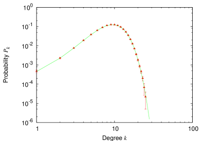
Figure 1: The degree distribution for a network of $n=50\,000$ vertices generated using the biased random walk mechanism described in the text with $\mu=10$. The points represent the results of our simulations and the solid line is the target distribution, Eq. (32).

IV Example application

As an example of the application of these ideas we consider peer-to-peer networks. Bandwidth restrictions and search times place substantial constraints on the performance of peer-to-peer networks, and the methods of the previous sections can be used to nudge networks towards a structure that improves their performance in these respects. More sophisticated applications are certainly possible, but the one presented here offers an indication of the kinds of possibilities open to us.

IV.1 Definition of the problem

Consider a distributed database consisting of a set of computers each of which holds some data items. Copies of the same item can exist on more than one computer, which would make searching easier, but we will not assume this to be the case. Computers are connected together in a “virtual network,” meaning that each computer is designated as a “neighbor” of some number of other computers. These connections between computers are purely notional: every computer can communicate with every other directly over the Internet or other physical network. The virtual network is used only to limit the amount of information that computers have to keep about their peers.

Each computer maintains a directory of the data items held by its network neighbors, but not by any other computers in the network. Searches for items are performed by passing a request for a particular item from computer to computer until it reaches one in whose directory that item appears, meaning that one of that computer’s neighbors holds the item. The identity of the computer holding the item is then transmitted back to the origin of the search and the origin and target computers communicate directly thereafter to negotiate the transfer of the item. This basic model is essentially the same as that used by other authors ALPH01 as well as by many actual peer-to-peer networks in the real world. Note that it achieves efficiency by the use of relatively large directories at each vertex of the network, which inevitably use up memory resources on the computers. However, with standard hash-coding techniques and for databases of the typical sizes encountered in practical situations (thousands or millions of items) the amounts of memory involved are quite modest by modern standards.

IV.2 Search time and bandwidth

The two metrics of search performance that we consider in this example are search time and bandwidth, both of which should be low for a good search algorithm. We define the search time to be the number of steps taken by a propagating search query before the desired target item is found. We define the bandwidth for a vertex as the average number of queries that pass through that vertex per unit time. Bandwidth is a measure of the actual communications bandwidth that vertices must expend to keep the network as a whole running smoothly, but it is also a rough measure of the CPU time they must devote to searches. Since these are limited resources it is crucial that we not allow the bandwidth to grow too quickly as vertices are added to the network, otherwise the size of the network will be constrained, a severe disadvantage for networks that can in some cases swell to encompass a significant fraction of all the computers on the planet. (In some early peer-to-peer networks, issues such as this did indeed place impractical limits on network size Ritter00 ; RFI02 .)

Assuming that the average behavior of a user of the database remains essentially the same as the network gets larger, the number of queries launched per unit time should increase linearly with the size of the network, which in turn suggests that the bandwidth per vertex might also increase with network size, which would be a bad thing. As we will show, however, it is possible to avoid this by designing the topology of the network appropriately.

IV.3 Search strategies and search time

In order to treat the search problem quantitatively, we need to define a search strategy or algorithm. Here we consider a very simple—even brainless—strategy, again employing the idea of a random walk. This random walk search is certainly not the most efficient strategy possible, but it has two significant advantages for our purposes. First, it is simple enough to allow us to carry out analytic calculations of its performance. Second, as we will show, even this basic strategy can be made to work very well. Our results constitute an existence proof that good performance is achievable: searches are necessarily possible that are at least as good as those analyzed here.

The definition of our random walk search is simple: the vertex $i$ originating a search sends a query for the item it wishes to find to one of its neighbors $j$, chosen uniformly at random. If that item exists in the neighbor’s directory the identity of the computer holding the item is transmitted to the originating vertex and the search ends. If not, then $j$ passes the query to one of its neighbors chosen at random, and so forth. (One obvious improvement to the algorithm already suggests itself: that $j$ not pass the query back to $i$ again. As we have said, however, our goal is simplicity and we will allow such “backtracking” in the interests of simplifying the analysis.)

We can study the behavior of this random walk search by a method similar to the one we employed for the analysis of the biased random walks of Section III. Let $p_{i}$ be the probability that our random walker is at vertex $i$ at a particular time. Then the probability $p_{i}^{\prime}$ of its being at $i$ one step later, assuming the target item has not been found, is

$$p_{i}^{\prime}=\sum_{j}{A_{ij}\over k_{j}}p_{j},$$ (34)

where $k_{j}$ is the degree of vertex $j$ and $A_{ij}$ is an element of the adjacency matrix, Eq. (27). Under the same conditions as before the probability distribution over vertices then tends to the fixed point of (34), which is at

$$p_{i}={k_{i}\over 2m},$$ (35)

where $m$ is the total number of edges in the network. That is, the random walk visits vertices with probability proportional to their degrees. (An alternative statement of the same result is that the random walk visits edges uniformly.)

When our random walker arrives at a previously unvisited vertex of degree $k_{i}$, it “learns” from that vertex’s directory about the items held by all immediate neighbors of the vertex, of which there are $k_{i}-1$ excluding the vertex we arrived from (whose items by definition we already know about). Thus at every step the walker gathers more information about the network. The average number of vertices it learns about upon making a single step is $\sum_{i}p_{i}(k_{i}-1)$, with $p_{i}$ given by (35), and hence the total number it learns about after $\tau$ steps is

$${\tau\over 2m}\sum_{i}k_{i}(k_{i}-1)=\tau\biggl{[}{\langle k^{2}\rangle\over\langle k\rangle}-1\biggr{]},$$ (36)

where $\langle k\rangle$ and $\langle k^{2}\rangle$ represent the mean and mean-square degrees in the network and we have made use of $2m=n\langle k\rangle$. (There is in theory a correction to this result because the random walker is allowed to backtrack and visit vertices visited previously. For a well-mixed walk, however, this correction is of order $1/\langle k\rangle$, which, as we will see, is negligible for the networks we will be considering.)

How long will it take our walker to find the desired target item? That depends on how many instances of the target exist in the network. In many cases of practical interest, copies of items exist on a fixed fraction of the vertices in the network, which makes for quite an easy search. We will not however assume this to be the case here. Instead we will consider the much harder problem in which copies of the target item exist on only a fixed number of vertices, where that number could potentially be just 1. In this case, the walker will need to learn about the contents of $\mathrm{O}(n)$ vertices in order to find the target and hence the average time to find the target is given by

$$\tau\biggl{[}{\langle k^{2}\rangle\over\langle k\rangle}-1\biggr{]}=An,$$ (37)

for some constant $A$, or equivalently,

$$\tau=A{n\over\langle k^{2}\rangle/\langle k\rangle-1}.$$ (38)

Consider, for instance, a network with a power-law degree distribution of the form, $p_{k}=Ck^{-\gamma}$, where $\gamma$ is a positive exponent and $C$ is a normalizing constant chosen such that $\sum_{k=0}^{\infty}p_{k}=1$. Real-world networks usually exhibit power-law behavior only over a certain range of degree. Taking the minimum of this range to be $k=1$ and denoting the maximum by $k_{\mathrm{max}}$, we have

$${\langle k^{2}\rangle\over\langle k\rangle}\sim-\frac{k_{\mathrm{max}}^{3-\gamma}-1}{k_{\mathrm{max}}^{2-\gamma}-1}.$$ (39)

Typical values of the exponent $\gamma$ fall in the range $2<\gamma<3$, so that $k_{\mathrm{max}}^{2-\gamma}$ is small for large $k_{\mathrm{max}}$ and can be ignored. On the other hand, $k_{\mathrm{max}}^{3-\gamma}$ becomes large in the same limit and hence $\langle k^{2}\rangle/\langle k\rangle\sim k_{\mathrm{max}}^{3-\gamma}$ and

$$\tau\sim nk_{\mathrm{max}}^{\gamma-3}.$$ (40)

The scaling of the search time with system size $n$ thus depends, in this case, on the scaling of the maximum degree $k_{\mathrm{max}}$.

As an example, Aiello et al. ACL00 studied power-law degree distributions with a cut-off of the form $k_{\mathrm{max}}\sim n^{1/\gamma}$, which gives

$$\tau\sim n^{2-3/\gamma}.$$ (41)

A similar result was obtained previously by Adamic et al. ALPH01 using different methods.

IV.4 Bandwidth

Bandwidth is the mean number of queries reaching a given vertex per unit time. Equation (35) tells us that the probability that a particular current query reaches vertex $i$ at a particular time is $k_{i}/2m$, and assuming as discussed above that the number of queries initiated per unit time is proportional to the total number of vertices, the bandwidth for vertex $i$ is

$$Bn{k_{i}\over 2m}=B{k_{i}\over\langle k\rangle},$$ (42)

where $B$ is another constant.

This implies that high-degree vertices will be overloaded by comparison with low-degree ones so that, despite their good performance in terms of search times, networks with power-law or other highly right-skewed degree distributions may be undesirable in terms of bandwidth, with bottlenecks forming around the vertices of highest degree that could harm the performance of the entire network. If we wish to distribute load more evenly among the computers in our network, a network with a tightly peaked degree distribution is desirable.

IV.5 Choice of network

A simple and attractive choice for our network is the Poisson distributed network of Section III. For a Poisson degree distribution with mean $\mu$ we have $\langle k\rangle=\mu$ and $\langle k^{2}\rangle=\mu^{2}+\mu$. Then, using Eq. (38), the average search time is

$$\tau=A{n\over\mu}.$$ (43)

As we have seen, a network of this type can be realized in practice with a biased-random-walker attachment mechanism of the kind described in Section III.

Now if we allow $\mu$ to grow as some power of the size of the entire network, $\mu\sim n^{\alpha}$ with $0\leq\alpha\leq 1$, then $\tau\sim n^{1-\alpha}$. For smaller values of $\alpha$, searches will take longer, but vertices’ degrees are lower on average meaning that each vertex will have to devote less memory resources to maintaining its directory. Conversely, for larger $\alpha$, searches will be completed more quickly at the expense of greater memory usage. In the limiting case $\alpha=1$, searches are completed in constant time, independent of the network size, despite the simple-minded nature of the random walk search algorithm.

The price we pay for this good performance is that the network becomes dense, having a number of edges scaling as $n^{1+\alpha}$. It is important to bear in mind, however, that this is a virtual network, in which the edges are a purely notional construct whose creation and maintenance carries essentially zero cost. There is a cost associated with the directories maintained by vertices, which for $\alpha=1$ will contain information on the items held by a fixed fraction of all the vertices in the network. For instance, each vertex might be required to maintain a directory of 1% of all items in the network. Because of the nature of modern computer technology, however, we don’t expect this to create a significant problem. User time (for performing searches) and CPU time and bandwidth are scarce resources that must be carefully conserved, but memory space on hard disks is cheap, and the tens or even hundreds of megabytes needed to maintain a directory is considered in most cases to be a small investment. By making the choice $\alpha=1$ we can trade cheap memory resources for essentially optimal behavior in terms of search time and this is normally a good deal for the user.

We note also that the search process is naturally parallelizable: there is nothing to stop the vertex originating a search from sending out several independent random walkers and the expected time to complete the search will be reduced by a factor of the number of walkers. Alternatively, we could reduce the degrees of all vertices in the network by a constant factor and increase the number of walkers by the same factor, which would keep the average search time constant while reducing the sizes of the directories substantially, at the cost of increasing the average bandwidth load on each vertex.

As a test of our proposed search scheme, we have performed simulations of the procedure on Poisson networks generated using the random-walker method of Section III. Figure 2 shows as a function of network size the average time $\tau$ taken by a random walker to find an item placed at a single randomly chosen vertex in the network. As we can see, the value of $\tau$ does indeed tend to a constant (about 100 steps in this case) as network size becomes large.

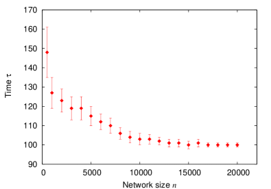
Figure 2: The time $\tau$ for the random walk search to find an item deposited at a random vertex, as a function of the number of vertices $n$.

We should also point out that for small values of $\mu$ vertices with degree zero could cause a problem. A vertex that loses all of its edges because its neighbors have all left the network can no longer be reached by our random walkers, and hence no vertices can attach to them and our attachment scheme breaks down. However, in the case considered here, where $\mu$ becomes large, the number of such vertices is exponentially small, and hence they can be neglected without substantial deleterious effects. Any vertex that does find itself entirely disconnected from the network can simply rejoin by the standard mechanism.

IV.6 Item frequency distribution

In most cases, the search problem posed above is not a realistic representation of typical search problems encountered in peer-to-peer networks. In real networks, copies of items often occur in many places in the network. Let $s$ be the number of times a particular item occurs in the network and let $p_{s}$ be the probability distribution of $s$ over the network, i.e., $p_{s}$ is the fraction of items that exist in $s$ copies.

If the item we are searching for exists in $s$ copies, then Eq. (43) becomes

$$\tau_{s}=A{n\over\mu s},$$ (44)

since the chance of finding a copy of the desired item is multiplied by $s$ on each step of the random walk. On the other hand, it is likely that the frequency of searches for items is not uniformly distributed: more popular items, that is those with higher $s$, are likely to be searched for more often than less popular ones. For the purposes of illustration, let us make the simple assumption that the frequency of searches for a particular item is proportional to the item’s popularity. Then the average time taken by a search is

$$\langle\tau\rangle={\sum_{s=1}^{\infty}sp_{s}\tau_{s}\over\sum_{s=1}^{\infty}sp_{s}}=A{n\over\mu\langle s\rangle},$$ (45)

where we have made use of $\sum_{s}p_{s}=1$ and $\sum_{s}sp_{s}=\langle s\rangle$.

One possibility is that the total number of copies of items in the network increases in proportion to the number of vertices, but that the number of distinct items remains roughly the same, so that the average number of copies of a particular item increases as $\langle s\rangle\sim n$. In this case, $\langle\tau\rangle$ becomes independent of $n$ even when $\mu$ is constant, since we have to search only a constant number of vertices, not a constant fraction, to find a desired item. Perhaps a more realistic possibility is that the number of distinct items increases with network size, but does so slower than $n$, in which case one can achieve constant search times with a mean degree $\mu$ that also increases slower than $n$, so that directory sizes measured as a fraction of the network size dwindle.

An alternative scenario is one of items with a power-law frequency distribution $p_{s}\sim s^{-\delta}$. This case describes, for example, most forms of mass art or culture including books and recordings, emails and other messages circulating on the Internet, and many others Newman05b . The mean time to perform a search in the network then depends on the value of the exponent $\delta$. In many cases we have $\delta>2$, which means that $\langle s\rangle$ is finite and well-behaved as the database becomes large, and hence $\langle\tau\rangle$, Eq. (45), differs from Eq. (43) by only a constant factor. (That factor may be quite large, making a significant practical difference to the waiting time for searches to complete, but the scaling with system size is unchanged.) If $\delta<2$, however, then $\langle s\rangle$ becomes ill-defined, having a formally divergent value, so that $\langle\tau\rangle\to 0$ as system size becomes large. Physically, this represents the case in which most searches are for the most commonly occurring items, and those items occur so commonly that most searches terminate very quickly.

While this extra speed is a desirable feature of the search process, it’s worth noting that average search time may not be the most important metric of performance for users of the network. In many situations, worst-case search time is a better measure of the ability of the search algorithm to meet users’ demands. Assuming that the most infrequently occurring items in the network occur only once, or only a fixed number of times, the worst-case performance will still be given by Eq. (43).

IV.7 Estimating network size

One further detail remains to be considered. If we want to make the mean degree $\mu$ of vertices added to the network proportional to the size $n$ of the entire network, or to some power of $n$, we need to know $n$, which presents a challenge since, as we have said, we do not expect any vertex to know the identity of all or even most of the other the vertices. This problem can be solved using a breadth-first search, which can be implemented once again by message passing across the network. One vertex $i$ chosen at random (or more realistically every vertex, at random but stochastically constant intervals proportional to system size) sends messages to some number $d$ of randomly chosen neighbors. The message contains the address of vertex $i$, a unique identifier string, and a counter whose initial value is zero. Each receiving vertex increases the counter by 1, passes the message on to one of its neighbors, and also sends messages with the same address, identifier, and with counter zero to $d-1$ other neighbors. Any vertex receiving a message with an identifier it has seen previously sends the value of the counter contained in that message back to vertex $i$, but does not forward the message to any further vertices. If vertex $i$ adds together all of the counter values it receives, the total will equal the number of vertices (other than itself) in the entire network. This number can then be broadcast to every other vertex in the network using a similar breadth-first search (or perhaps as a part of the next such search instigated by vertex $i$.)

The advantage of this process is that it has a total bandwidth cost (total number of messages sent) equal to $dn$. For constant $d$ therefore, the cost per vertex is a constant and hence the process will scale to arbitrarily large networks without consuming bandwidth. The (worst-case) time taken by the process depends on the longest geodesic path between any two vertices in the network, which is $\mathrm{O}(\log n)$. Although not as good as $\mathrm{O}(1)$, this still allows the network to scale to exponentially large sizes before the time needed to measure network size becomes an issue, and it seems likely that directory size (which scales linearly with or as a power of $n$ depending on the precise algorithm) will become a limiting factor long before this happens.

V Conclusions

In this paper, we have considered the problem of designing networks indirectly by manipulating the rules by which they evolve. For certain types of networks, such as peer-to-peer networks, the limited control that this manipulation gives us over network structure, such as the ability to impose an arbitrary degree distribution of our choosing on the network, may be sufficient to generate significant improvements in network performance. Using generating function methods, we have shown that it is possible to impose a (nearly) arbitrary degree distribution on a network by appropriate choice of the “attachment kernel” that governs how newly added vertices connect to the network. Furthermore, we have described a scheme based on biased random walks whereby arbitrary attachment kernels can be implemented in practice.

We have also considered what particular choices of degree distribution offer the best performance in idealized networks under simple assumptions about search strategies and bandwidth constraints. We have given general formulas for search times and bandwidth usage per vertex and studied in detail one particularly simple case of a Poisson network that can be realized in straightforward fashion using our biased random walker scheme, allows us to perform decentralized searches in constant time, and makes only constant bandwidth demands per vertex, even in the limit where the database becomes arbitrarily large. No part of the scheme requires any centralized knowledge of the network, making the network a true peer-to-peer network, in the sense of having client nodes only and no servers.

One important issue that we have neglected in our discussion is that of “supernodes” in the network. Because the speed of previous search strategies has been recognized as a serious problem for peer-to-peer networks, designers of some networks have chosen to designate a subset of network vertices (typically those with above-average bandwidth and CPU resources) as supernodes. These supernodes are themselves connected together into a network over which all search activity takes place. Other client vertices then query this network when they want a search performed. Since the size of the supernode network is considerably less than the size of the network as a whole, this tactic increases the speed of searches, albeit only by a constant factor, at the expense of heavier load on the supernode machines. It would be elementary to generalize our approach to incorporate supernodes. One would simply give each supernode a directory of the data items stored by the client vertices of its supernode neighbors. Then searches would take place exactly as before, but on the supernode network alone, and client vertices would query the supernode network to perform searches. In all other respects the mechanisms would remain the same.

- (1) M. E. J. Newman, The structure and function of complex networks. SIAM Review 45, 167–256 (2003).
- (2) S. Boccaletti, V. Latora, Y. Moreno, M. Chavez, and D.-U. Hwang, Complex networks: Structure and dynamics. Physics Reports 424, 175–308 (2006).
- (3) S. N. Dorogovtsev and J. F. F. Mendes, Evolution of Networks: From Biological Nets to the Internet and WWW. Oxford University Press, Oxford (2003).
- (4) M. E. J. Newman, A.-L. Barabási, and D. J. Watts, The Structure and Dynamics of Networks. Princeton University Press, Princeton (2006).
- (5) G. Paul, T. Tanizawa, S. Havlin, and H. E. Stanley, Optimization of robustness of complex networks. Eur. Phys. J. B 38, 187–191 (2004).
- (6) L. A. Adamic, R. M. Lukose, A. R. Puniyani, and B. A. Huberman, Search in power-law networks. Phys. Rev. E 64, 046135 (2001).
- (7) N. Sarshar, P. O. Boykin, and V. P. Rowchowdhury, Scalable percolation search in power law networks. In Proceedings of the 4th International Conference on Peer-to-Peer Computing, pp. 2–9, IEEE Computer Society, New York (2004).
- (8) T. Hong, Performance. In A. Oram (ed.), Peer-to-Peer: Harnessing the Benefits of a Disruptive Technology, pp. 203–241, O’Reilly and Associates, Sebastopol, CA (2001).
- (9) P. L. Krapivsky and S. Redner, Organization of growing random networks. Phys. Rev. E 63, 066123 (2001).
- (10) C. Moore, G. Ghoshal, and M. E. J. Newman, Exact solutions for models of evolving networks with addition and deletion of nodes. Phys. Rev. E 74, 036121 (2006).
- (11) M. E. J. Newman, S. H. Strogatz, and D. J. Watts, Random graphs with arbitrary degree distributions and their applications. Phys. Rev. E 64, 026118 (2001).
- (12) N. Sarshar and V. Roychowdhury, Scale-free and stable structures in complex ad hoc networks. Phys. Rev. E 69, 026101 (2004).
- (13) C. Cooper, A. Frieze, and J. Vera, Random deletion in a scale-free random graph process. Internet Mathematics 1, 463–483 (2004).
- (14) J. P. Ritter, Why Gnutella can’t scale. No, really (2000), URL http://www.darkridge.com/~jpr5/doc/gnutella.html.
- (15) M. Ripeanu, I. Foster, and A. Iamnitchi, Mapping the Gnutella network: Properties of large-scale peer-to-peer systems and implications for system design. IEEE Internet Computing 6, 50–57 (2002).
- (16) W. Aiello, F. Chung, and L. Lu, A random graph model for massive graphs. In Proceedings of the 32nd Annual ACM Symposium on Theory of Computing, pp. 171–180, Association of Computing Machinery, New York (2000).
- (17) M. E. J. Newman, Power laws, Pareto distributions and Zipf’s law. Contemporary Physics 46, 323–351 (2005).