Fractal Analysis of River Flow Fluctuations

Abstract

We use some fractal analysis methods to study river flow fluctuations. The result of the Multifractal Detrended Fluctuation Analysis (MF-DFA) shows that there are two crossover timescales at $s_{1\times}\sim 12$ and $s_{2\times}\sim 130$ months in the fluctuation function. We discuss how the existence of the crossover timescales are related to a sinusoidal trend. The first crossover is due to the seasonal trend and the value of second ones is approximately equal to the well known cycle of sun activity. Using Fourier detrended fluctuation analysis, the sinusoidal trend is eliminated. The value of Hurst exponent of the runoff water of rivers without the sinusoidal trend shows a long range correlation behavior. For the Daugava river the value of Hurst exponent is $0.52\pm 0.01$ and also we find that these fluctuations have multifractal nature. Comparing the MF-DFA results for the remaining data set of Daugava river to those for shuffled and surrogate series, we conclude that its multifractal nature is almost entirely due to the broadness of probability density function.

Keywords: Time series, Fractal analysis, River flow, Long-range correlation, Hurst exponent

]

I Introduction

Interpretation and estimation of climate change has been one of the main research areas in science [1, 2, 3]. The climate system often exhibits irregular and complex behavior. Although the climate system is driven by the well-defined seasonal periodicity, it is also a subject to unpredictable perturbations which can lead to extreme climate events. Indeed the climate is a dynamical system influenced by immense factors, such as solar radiation or the topography of the surface of the solid earth, etc. All factors that control the trajectory of climate have enormously large phase space, thus we have to analysis it with stochastic tools. Several recent statistical studies have shown that a remarkably wide variety of natural systems display fluctuations that may be characterized by long-range power-law correlations. Such correlations hint toward fractal geometry of the underlying dynamical system. Existence and determination of power-law correlations would help to quantify the underlying process dynamics [4, 5].

The analysis of river flows has a long history, nevertheless some important issues have been lost. Here, we study one component of the climate system, the river flux, by using the novel approach in the fractal analysis like Detrended Fluctuation Analysis, Fourier-Detrended Fluctuation Analysis and Scaled Windowed Variance Analysis Methods. The statistical and fractal analysis of river flows should be an important issue in the geophysics and hydrological systems to recognize the influence of environmental conditions and to detect relative effects. A set of most important results which can be given by using statistical tools is as follows: a concept of scale self-similarity for the topography of Earth’s surface [6], the hydraulic-geometric similarity of river system and floods forced by the heavy rain [7, 8], etc. Already more than half a century ago the engineer Hurst found that runoff records from various rivers exhibit ’long-range statistical dependencies’[9]. Later, such long-term correlated fluctuation behavior has also been reported for many other geophysical records including precipitation data [6, 10, 11]. These original approaches exclusively focused on the absolute values or the variances of the full distribution of the fluctuations, which can be regarded as the first and second moments of detrended fluctuation analysis [6, 9, 10, 12]. In the last decade it has been realized that a multifractal description is required for a full characterization of the runoff records [13, 14]. This multifractal description of the records can be regarded as a ’fingerprint’ for each station or river, which, among other things, can serve as an efficient non-trivial test bed for the state-of-the-art precipitation-runoff models.

River flow can be characterized by several general features. As a result of the periodicity in precipitation, river flow has also strong seasonal periodicity. The seasonal cycle of river flow is asymmetric; i.e., river flow increases rapidly (usually during late winter and spring) and decreases gradually (toward the end of the autumn). The fluctuations in river flow are large for large river flow and small for small river flow [5]. It is important to note that unlike other climate components, river flow may has a direct impact of human activity, like damming, use of river water for agriculture, etc., a fact which makes the river flow data more difficult to study. The fluctuations in river flow are of special interest since they are directly linked to floods and droughts. There are several interesting characteristics of river flow fluctuations: (i) the river flow fluctuations have power law tails in the probability distribution [15, 16], (ii) the river flow fluctuations are long-range correlated [9, 17, 18], and (iii) river flow fluctuations are multifractal [13, 14, 19]. The scaling laws may improve the statistical prediction of extreme changes in river flow [20]. Recently connection between volatility and nonlinearity has originally been established by [21, 22], the degree of non-linearity has been checked using the volatility series, also a simple model of river fluctuations has been determined [4, 5]. More recently the annual runoff for the Ukrainian and Moldavia’s rivers and reveal scale invariance for distribution of this variable have been investigated by using statistical parameters such as arithmetic average, coefficients of variation, skewness, and auto-correlation [23]. In all of the previous researches, the contribution sinusoidal trends on the creation of crossover in the results of fractal analysis and the multifractal nature have been lost. The effect of nonstationarity on the detrended fluctuation analysis has been investigated [24]. In addition, the effects of periodic trends on the fractal scaling properties of a time series have been investigated moreover in some paper a relation between amplitude and the period of the periodic trends and the existence of crossover in the Detrended Fluctuations scaling function have been demonstrated [24]. So the main purpose of this paper are the investigation of the effects of seasonal trend on the multifractal analysis of flow fluctuations and determination of the source of multifractality in data . For completeness of this investigation and to get the deep insight of the contribution of sun activity in the statistical properties of river flow, we compare the recent fractal analysis results of sunspots [25] with current analysis. The Sunspot number was collected by the Sunspot Index Data Center (SIDC) [26]. Due to the stochastic nature of river flow, it is probable that the sun activity may affects on the duct of river, so to demonstrate the presence of any correlations we compare results of river flow and sun activity extracted by various fractal analysis. It was well-known that the statistical properties of every rivers depend on very important reasons which affect on flow fluctuations, so one can not expect that the sun activity has a same reasonable effect on different rivers.

In addition we would like to characterize the complex behavior of the monthly runoff for the Daugava river fluctuations through the computation of the signal parameters - scaling exponents - which quantifies the correlation exponents and multifractality of the signal. We investigate the correlation behavior of duct river time series which is governed by power-law.

The original Daugava river data source is Latvian Environmental Geological and Meteorological Agency database. They describe water flow through hydroelectric power station near Ķegums, Latvia. Dimension of the data is m³/s. Other data which are used here are from National Water Information System: Web Interface [27]. As shown in the upper panel of Figure 1, the duct water of Daugava river series has a sinusoidal trend, with a dominant frequency. These trends should involve the seasonal and other physical reasons in natural phenomenon. Because of the complexity nature of river flow series, and due to the finiteness of the available data sample, we should apply some methods which are insensitive to non-stationarities like trends. To eliminate the effect of sinusoidal trend, we apply the Fourier Detrended Fluctuation Analysis (F-DFA) [28, 29]. After elimination of the trend we use the Multifractal Detrended Fluctuation Analysis (MF-DFA) to analysis the data set. The MF-DFA methods are the modified version of detrended fluctuation analysis (DFA) to detect multifractal properties of time series. The detrended fluctuation analysis (DFA) method introduced by Peng et al. [30] has became a widely-used technique for the determination of (multi-) fractal scaling properties and the detection of long-range correlations in noisy, nonstationary time series [24, 30, 31, 32, 33]. It has successfully been applied to diverse fields such as DNA sequences [30, 34], heart rate dynamics [35, 36, 37], neuron spiking [38], human gait [39], long-time weather records [40], cloud structure [41], geology [42], ethnology [43], economical time series [44, 45], solid state physics [46], sunspot time series [25] and cosmic microwave background radiation [47].

This paper is organized as follows: In Section II we describe the MF-DFA, F-DFA and Scale Windowed Variance (SWV) methods in detail and show that the scaling exponents determined via the MF-DFA method are identical to those obtained by the standard multifractal formalism based on partition functions. We eliminate the sinusoidal trend via the F-DFA technique in Section III and investigate the multifractal nature of the remaining fluctuation, we use certain fractal analysis approaches such as, the Multifractal Detrended Fluctuation Analysis (MF-DFA), and Scaled Windowed Variance (SWV) to analysis the data set, The DFA result of sun activity and river flows are compared together. In Section IV, we examine the source of multifractality in duct water of Daugava river data by comparison the MF-DFA results for remaining data set to those obtained via the MF-DFA for shuffled and surrogate series. Section V closes with a discussion of the present results.

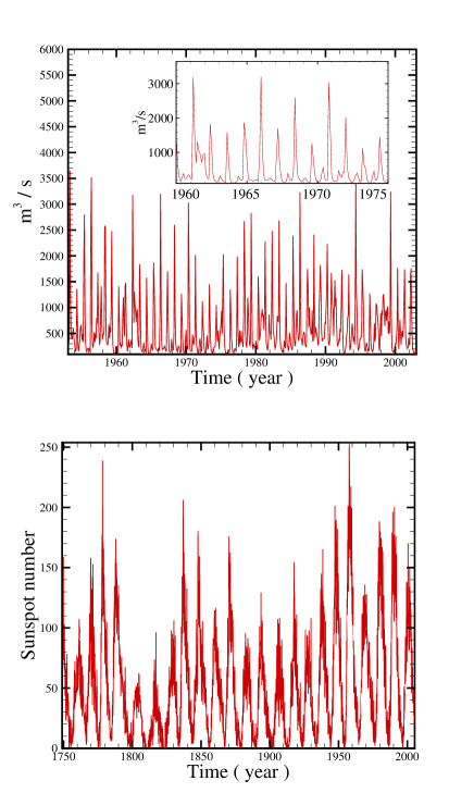
FIG. 1.: Observed flux series of Daugava river (upper panel) and Sunspot number (lower panel) as a function of time.

II Fractal Analysis Methods

In this section we introduce three methods to investigate the fractal properties of stochastic processes.

A Multifractal Detrended Fluctuation Analysis

The simplest type of the multifractal analysis is based upon the standard partition function multifractal formalism, which has been developed for the multifractal characterization of normalized, stationary measurements [48, 49, 50, 51]. Unfortunately, this standard formalism does not give correct results for nonstationary time series that are affected by trends or that cannot be normalized. Thus, in the early 1990s an improved multifractal formalism has been developed, the wavelet transform modulus maxima (WTMM) method [52], which is based on the wavelet analysis and involves tracing the maxima lines in the continuous wavelet transform over all scales. The other method, the multifractal detrended fluctuation analysis (MF-DFA), is based on the identification of scaling of the $q$th-order moments depending on the signal length and is generalization of the standard DFA using only the second moment $q=2$.

The MF-DFA does not require the modulus maxima procedure in contrast WTMM method, and hence does not require more effort in programming and computing than the conventional DFA. On the other hand, often experimental data are affected by non-stationarities like trends, which have to be well distinguished from the intrinsic fluctuations of the system in order to find the correct scaling behavior of the fluctuations. In addition very often we do not know the reasons for underlying trends in collected data and even worse we do not know the scales of the underlying trends, also, usually the available record data is small. For the reliable detection of correlations, it is essential to distinguish trends from the fluctuations intrinsic in the data. Hurst rescaled-range analysis [10] and other non-detrending methods work well if the records are long and do not involve trends. But if trends are present in the data, they might give wrong results. Detrended fluctuation analysis (DFA) is a well-established method for determining the scaling behavior of noisy data in the presence of trends without knowing their origin and shape [30, 36, 53, 54, 55]. Also DFA scaling results are not immune to different trends and to different artifacts such as spikes, missing segments of data etc. [33, 56, 57].

In spite of many abilities of this method, in some cases is encountered with problem and gives wrong results. DFA method can only determine positive Hurst exponent, $H$, and gives an inaccurate results for strongly anti-correlated record data when $H$ is close to zero. To avoid this situation, in such case one should use the integrated data. This signal is so-called double profiled data set. The corresponding Hurst exponent using this way is $H=\bar{H}-1$, here $\bar{H}$ is derived from DFA method for the double profiled signals [25, 58]. According to the recent exploration in ref. [32], a deviation in the DFA results occurs in very short records and in the small regime of data in each window mentioned in the forthcoming subsection. The modified version of MF-DFA will be used for these cases [32]. In this paper also we will introduce this method and apply to infer correct exponent for river flow fluctuations.

B Description of the MF-DFA

The modified multifractal DFA (MF-DFA) procedure consists of five steps[58] . The first three steps are essentially identical to the conventional DFA procedure (see e. g. [24, 30, 31, 32, 33]). Suppose that $x_{k}$ is a series of length $N$, and that this series is of compact support, i.e. $x_{k}=0$ for an insignificant fraction of the values only.

$\bullet$ Step 1: Determine the “profile”

$$Y(i)\equiv\sum_{k=1}^{i}\left[x_{k}-\langle x\rangle\right],\qquad i=1,\ldots,N.$$ (1)

Subtraction of the mean $\langle x\rangle$ is not compulsory, since it would be eliminated by the later detrending in the third step.

$\bullet$ Step 2: Divide the profile $Y(i)$ into $N_{s}\equiv{\rm int}(N/s)$ non-overlapping segments of equal lengths $s$. Since the length $N$ of the series is often not a multiple of the considered time scale $s$, a short part at the end of the profile may remain. In order not to disregard this part of the series, the same procedure is repeated starting from the opposite end. Thereby, $2N_{s}$ segments are obtained altogether.

$\bullet$ Step 3: Calculate the local trend for each of the $2N_{s}$ segments by a least-square fit of the series. Then determine the variance

$$F^{2}(s,\nu)\equiv{1\over s}\sum_{i=1}^{s}\left\{Y[(\nu-1)s+i]-y_{\nu}(i)\right\}^{2},$$ (2)

for each segment $\nu$, $\nu=1,\ldots,N_{s}$ and

$$F^{2}(s,\nu)\equiv{1\over s}\sum_{i=1}^{s}\left\{Y[N-(\nu-N_{s})s+i]-y_{\nu}(i)\right\}^{2},$$ (3)

for $\nu=N_{s}+1,\ldots,2N_{s}$. Here, $y_{\nu}(i)$ is the fitting polynomial in segment $\nu$. Linear, quadratic, cubic, or higher order polynomials can be used in the fitting procedure (conventionally called DFA1, DFA2, DFA3, $\ldots$) [30, 37]. Since the detrending of the time series is done by the subtraction of the polynomial fits from the profile, different order DFA differ in their capability of eliminating trends in the series. In (MF-)DFA$m$ [$m$th order (MF-)DFA] trends of order $m$ in the profile (or, equivalently, of order $m-1$ in the original series) are eliminated. Thus a comparison of the results for different orders of DFA allows one to estimate the type of the polynomial trend in the time series [24, 32].

$\bullet$ Step 4: Average over all segments to obtain the $q$-th order fluctuation function, defined as:

$$F_{q}(s)\equiv\left\{{1\over 2N_{s}}\sum_{\nu=1}^{2N_{s}}\left[F^{2}(s,\nu)\right]^{q/2}\right\}^{1/q},$$ (4)

where, in general, the index variable $q$ can take any real value except zero. For $q=2$, the standard DFA procedure is retrieved. Generally we are interested in how the generalized $q$ dependent fluctuation functions $F_{q}(s)$ depend on the time scale $s$ for different values of $q$. Hence, we must repeat steps 2, 3 and 4 for several time scales $s$. It is apparent that $F_{q}(s)$ will increase with increasing $s$. Of course, $F_{q}(s)$ depends on the DFA order $m$. By construction, $F_{q}(s)$ is only defined for $s\geq m+2$.

$\bullet$ Step 5: Determine the scaling behavior of the fluctuation functions by analyzing log-log plots of $F_{q}(s)$ versus $s$ for each value of $q$. If the series $x_{i}$ are long-range power-law correlated, $F_{q}(s)$ increases, for large values of $s$, as a power-law,

$$F_{q}(s)\sim s^{h(q)}.$$ (5)

In general, the exponent $h(q)$ may depend on $q$. For stationary time series such as fGn (fractional Gaussian noise), $Y(i)$ in Eq. 1, will be a fBm (fractional Brownian motion) signal, so, $0<h(q=2)<1.0$ (see the appendix for more details). The exponent $h(2)$ is identical to the well-known Hurst exponent $H$ [30, 31, 48]. Also for a nonstationary signal, such as fBm noise, $Y(i)$ in Eq. 1, will be a sum of fBm signal, so the corresponding scaling exponent of $F_{q}(s)$ is identified by $h(q=2)>1.0$ [30, 59]. In this case the relation between the exponents $h(2)$ and $H$ will be $H=h(q=2)-1$ (see appendix of [25]). The exponent $h(q)$ is known as generalized Hurst exponent. The auto-correlation function can be characterized by a power law $C(s)\equiv\langle n_{k}n_{k+s}\rangle\sim s^{-\gamma}$ with exponent $\gamma=2-2H$. Its power spectra can be characterized by $S(\omega)\sim\omega^{-\beta}$ with frequency $\omega$ and $\beta=2H-1$. In the nonstationary case, correlation function is (see appendix for more details):

$$C(i,j)=\langle n_{i}n_{j}\rangle\sim i^{2H}+j^{2H}-|i-j|^{2H}$$ (6)

and corresponding power spectrum scaling is $\beta=2H+1$ [25, 30, 59].

For monofractal time series, $h(q)$ is independent of $q$, since the scaling behavior of the variances $F^{2}(s,\nu)$ is identical for all segments $\nu$, and the averaging procedure in Eq. (4) will just give this identical scaling behavior for all values of $q$. If we consider positive values of $q$, the segments $\nu$ with large variance $F^{2}(s,\nu)$ (i. e. large deviations from the corresponding fit) will dominate the average $F_{q}(s)$. Thus, for positive values of $q$, $h(q)$ describes the scaling behavior of the segments with large fluctuations. For negative values of $q$, the segments $\nu$ with small variance $F^{2}(s,\nu)$ will dominate the average $F_{q}(s)$. Hence, for negative values of $q$, $h(q)$ describes the scaling behavior of the segments with small fluctuations [60].

1 Relation to standard multifractal analysis

For a stationary, normalized series the multifractal scaling exponents $h(q)$ defined in Eq. (5) are directly related to the scaling exponents $\tau(q)$ defined by the standard partition function-based multifractal formalism as shown below [58]. Suppose that the series $x_{k}$ of length $N$ is a stationary, normalized sequence. Then the detrending procedure in step 3 of the MF-DFA method is not required, since no trend has to be eliminated. Thus, the DFA can be replaced by the standard Fluctuation Analysis (FA), which is identical to the DFA except for a simplified definition of the variance for each segment $\nu$, $\nu=1,\ldots,N_{s}$. Step 3 now becomes [see Eq. (2)]:

$$F_{\rm FA}^{2}(s,\nu)\equiv[Y(\nu s)-Y((\nu-1)s)]^{2}.$$ (7)

Inserting this simplified definition into Eq. (4) and using Eq. (5), we obtain

$$\left\{{1\over 2N_{s}}\sum_{\nu=1}^{2N_{s}}|Y(\nu s)-Y((\nu-1)s)|^{q}\right\}^{1/q}\sim s^{h(q)}.$$ (8)

For simplicity we can assume that the length $N$ of the series is an integer multiple of the scale $s$, obtaining $N_{s}=N/s$ and therefore

$$\sum_{\nu=1}^{N/s}|Y(\nu s)-Y((\nu-1)s)|^{q}\sim s^{qh(q)-1}.$$ (9)

This corresponds to the multifractal formalism used e. g. in [49, 51]. In fact, a hierarchy of exponents $H_{q}$ similar to our $h(q)$ has been introduced based on Eq. (9) in [49]. In order to relate also to the standard textbook box counting formalism [48, 50], we employ the definition of the profile in Eq. (1). It is evident that the term $Y(\nu s)-Y((\nu-1)s)$ in Eq. (9) is identical to the sum of the numbers $x_{k}$ within each segment $\nu$ of size $s$. This sum is known as the box probability $p_{s}(\nu)$ in the standard multifractal formalism for normalized series $x_{k}$,

$$p_{s}(\nu)\equiv\sum_{k=(\nu-1)s+1}^{\nu s}x_{k}=Y(\nu s)-Y((\nu-1)s).$$ (10)

The scaling exponent $\tau(q)$ is usually defined via the partition function $Z_{q}(s)$,

$$Z_{q}(s)\equiv\sum_{\nu=1}^{N/s}|p_{s}(\nu)|^{q}\sim s^{\tau(q)},$$ (11)

where $q$ is a real parameter as in the MF-DFA method, discussed above. Using Eq. (10) we see that Eq. (11) is identical to Eq. (9), and obtain analytically the relation between the two sets of multifractal scaling exponents,

$$\tau(q)=qh(q)-1.$$ (12)

Thus, we observe that $h(q)$ defined in Eq. (5) for the MF-DFA is directly related to the classical multifractal scaling exponents $\tau(q)$. Note that $h(q)$ is different from the generalized multifractal dimensions

$$D(q)\equiv{\tau(q)\over q-1}={qh(q)-1\over q-1},$$ (13)

that are used instead of $\tau(q)$ in some papers. While $h(q)$ is independent of $q$ for a monofractal time series, $D(q)$ depends on $q$ in this case. Another way to characterize a multifractal series is the singularity spectrum $f(\alpha)$, that is related to $\tau(q)$ via a Legendre transform [48, 50],

$$\alpha=\tau^{\prime}(q)\quad{\rm and}\quad f(\alpha)=q\alpha-\tau(q).$$ (14)

Here, $\alpha$ is the singularity strength or Hölder exponent, while $f(\alpha)$ denotes the dimension of the subset of the series that is characterized by $\alpha$. Using Eq. (12), we can directly relate $\alpha$ and $f(\alpha)$ to $h(q)$,

$$\alpha=h(q)+qh^{\prime}(q)\quad{\rm and}\quad f(\alpha)=q[\alpha-h(q)]+1.$$ (15)

A Hölder exponent denotes monofractality, while in the multifractal case, the different parts of the structure are characterized by different values of $\alpha$, leading to the existence of the spectrum $f(\alpha)$.

C Fourier-Detrended Fluctuation Analysis

Many signals in the nature do not distinguished as monofractal scaling behavior. In some cases, there exist one or more crossover (time) scales $s_{\times}$ segregating regimes with different scaling exponents e.g long range correlation for $s\ll s_{\times}$ and an other type of correlation or uncorrelated behavior for $s\gg s_{\times}$ [24, 32]. In other cases investigation of the scaling behavior is more complicated. In the presence of different behavior of various moments in the MF-DFA method, different scaling exponents are required for different parts of the series [33]. Therefore one needs a multitude of scaling exponents (multifractality) for a full description of the scaling behavior. A crossover usually can arise from a change in the correlation properties of the signal at different time or space scales, or can often arise from trends in the data. To remove the crossover due to a trend such as sinusoidal trends, Fourier-Detrended Fluctuation Analysis (F-DFA) is applied. The F-DFA is a modified approach for the analysis of low frequency trends added to a noise in time series [28, 29, 61, 62].

In order to investigate how we can remove trends having a low frequency periodic behavior, we transform data record to Fourier space, then we truncate the first few coefficient of the Fourier expansion and inverse Fourier transform the series. After removing the sinusoidal trends we can obtain the fluctuation exponent by using the direct calculation of the MF-DFA. If truncation numbers are sufficient, The crossover due to a sinusoidal trend in the log-log plot of $F_{q}(s)$ versus $s$ disappears.

D Scaled Windowed Variance Analysis

The Scaled Windowed Variance analysis was developed by Cannon et al. (1997)[59]. The profile of data, $Y(i)$, is divided into $N_{s}\equiv{\rm int}(N/s)$ non-overlapping segments of equal lengths $s$. Then the standard deviation is calculated within each interval using the following relation

$${\rm SWV}(s)=\left(\frac{1}{s}\sum_{i=1}^{s}[Y(i)-\langle Y(s)\rangle]^{2}\right)^{1/2}.$$ (16)

The average standard deviation of all windows of length $s$ is computed. This computation is repeated over all possible interval lengths. The scaled windowed variance is related to $s$ by a power law

$${\rm SWV}\sim s^{H}.$$ (17)

III Analysis of data

As mentioned in section II, a spurious of correlations may be detected if time series is nonstationarity, so direct calculation of correlation behavior, spectral density exponent, fractal dimensions etc., don’t give the reliable results. It can be checked that the runoff for Daugava river is or not nonstationary. One can verified the non-stationarity property experimentally by measuring the stability of the average and variance in a moving window for example with scale $s$. Figure 2 shows the standard deviation of Daugava flow signal versus scale $s$, is saturated. Let us determine that whether the data set has a sinusoidal trend or not. According to the MF-DFA1 method, Generalized Hurst exponents $h(q)$ in Eq. (5) can be found by analyzing log-log plots of $F_{q}(s)$ versus $s$ for each $q$. Our investigation shows that there are at least two crossover time scales $s_{\times}$ in the log-log plots of $F_{q}(s)$ versus $s$ for every $q$’s. These two crossovers divide $F_{q}(s)$ into three regions, as shown in Figure 3 ( for instance we took $q=2$). Figure 4 shows these crossover also exist in the fluctuation function for various moments. The existence of these regions is due to the competition between noise and sinusoidal trend [24]. For $s<s_{1\times}$, the noise has the dominating effect . For $s_{1\times}<s<s_{2\times}$ the sinusoidal (such as seasonal) trend dominates [24]. The values of $s_{1\times}$ and $s_{2\times}$ are approximately equal to $12$ and $130$ months, respectively. The first crossover is clearly related to seasonal trend and the second ones is approximately equal to the well known cycle of sun activity. This shows that in addition of seasonal effect on the river flow, the sun activity strictly affects on the feature and fractal properties of river flow fluctuations. As shown in Figure 3, by comparing curves from some rivers and Sunspot we can see a certain symmetry in the form of curves. Points of inflection are placed closely, but angle of bendings are opposite (e.g. for Daugava river). This symmetry indicates a connection between the activity of sun and flow of water in the rivers. In both cases sinusoidal tendency have been found in the average part of the curves. Apparently the sun activity governs the rivers.

As mentioned before, for very small scales $s<s_{1\times}$ the effect of the sinusoidal trend is not pronounced, indicating that in this scale region the signal can be considered as noise fluctuating around a constant which is filtered out by the MF-DFA1 procedure. In this region the generalized DFA1 exponent for used rivers in this paper are listed in Figure 5 , where confirms that the process is a stationary process with long-range correlation behavior.

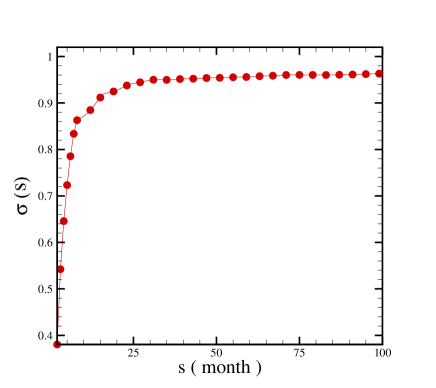
FIG. 2.: Behavior of standard deviation of duct of water as a function of time scale. It shows that this time series is stationary.

To cancel the sinusoidal trend in MF-DFA1, we apply F-DFA method on the present data. We truncate some of the first coefficients of the Fourier expansion of the river flow fluctuations. According to Figure 6, for eliminating the crossover scales, we need to remove approximately the first $200$ terms of the Fourier expansion. Then, by inverse Fourier Transformation, the noise without sinusoidal trend is extracted (see Figure 6) [28, 29, 61, 62].

The MF-DFA1 results of the remanning new signal just for Daugava river are shown in Figure 7. All exponent in this figure are driven at as maximum scale as possible in the log-log plots of $F_{q}(s)$ as function of $s$ (see Appendix for more details). The duct water of Daugava river series is a multifractal process as indicated by the strong $q$ dependence of generalized Hurst exponents and $\tau(q)$[58]. The $q$- dependence of the classical multifractal scaling exponent $\tau(q)$ has different behaviors for $q<0$ and $q>0$. For positive and negative values of $q$, the slopes of $\tau(q)$ are $0.45\pm 0.02$ and $1.17\pm 0.02$, respectively. According to the value of Hurst exponent, $H=0.52\pm 0.01$, we find that this series has approximately random behavior. This result is equal to value of Hurst exponent in small scale of MF-DFA1 of noise with sinusoidal trend. The values of derived quantities from MF-DFA1 method, are given in Table I. Using the SWV we also analysis the truncated series, Our result shows that the value of Hurst exponent is $H=0.50\pm 0.01$, which is in agreement with the previous result.

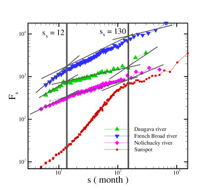
FIG. 3.: Crossover behavior of log-log plot $F(s)$ versus $s$ for some river flows and Sunspot series for $q=2.0$. For rivers there are at least two crossover time scales in plot of $F(s)$, at scales $s_{1\times}$ and $s_{2\times}$.

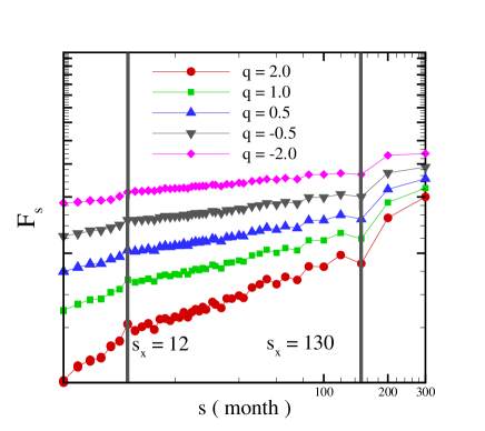
FIG. 4.: Crossover behavior of log-log plot $F(s)$ versus $s$ for Daugava river flow for various moments indicated on the figure. For river there are at least two crossover time scales in plot of $F(s)$, at scales $s_{1\times}$ and $s_{2\times}$. Vertical axis has arbitrary unite.

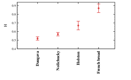
FIG. 5.: The values of Hurst exponent for some famous rivers.

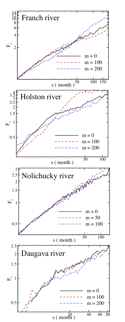
FIG. 6.: The MF-DFA1 functions $F_{2}(s)$ versus the time scale $s$ in log-log plot. Original time series $m=0$, truncation of $m=50$, $m=100$ and $m=200$ first terms.

Usually, in the MF-DFA method, deviation from a straight line in the log-log plot of Eq. (5) occurs for small scales $s$. This deviation limits the capability of DFA to determine the correct correlation behavior for very short scales and in the regime of small $s$. The modified MF-DFA is defined as follows [32]:

$$F^{\rm mod}_{q}(s) = \frac{F_{q}(s)}{K_{q}(s)},$$ (18)

$$= F_{q}(s){\langle[F_{q}^{\rm shuf}(s^{\prime})]^{2}\rangle^{1/2}\,s^{1/2}\over\langle[F_{q}^{\rm shuf}(s)]^{2}\rangle^{1/2}\,s^{\prime 1/2}}\quad{\rm(for}\,s^{\prime}\gg 1),$$ (19)

where $\langle[F_{q}^{\rm shuf}(s)]^{2}\rangle^{1/2}$ denotes the usual MF-DFA fluctuation function [defined in Eq. (4)] averaged over several configurations of shuffled data taken from the original time series, and $s^{\prime}\approx N/40$. The values of the Hurst exponent obtained by modified MF-DFA1 methods for duct water of Daugava river series is $0.54\pm 0.02$. The relative deviation of the Hurst exponent which is obtained by modified MF-DFA1 in comparison to MF-DFA1 for original data is approximately $3.84\%$. Now the value of Hurst exponent ensure us that the runoff fluctuations are long-range correlation, so by ignoring the seasonal trend, these processes have almost memory. This means that the status of runoff water statistically has long memory.

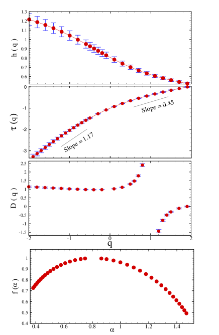
FIG. 7.: The $q$ dependence of the generalized Hurst exponent $h(q)$, the corresponding $\tau(q)$, generalized multifractal dimension $D(q)$ and singularity spectrum $f(\alpha)$ are shown in the upper to lower panel respectively for duct water of Daugava river series without sinusoidal trend.

IV Comparison of the multifractality for original, shuffled and surrogate series

As discussed in the section III the remanning data set after the elimination of sinusoidal trend has the multifractal nature. In this section we are interested in to determine the source of multifractality. In general, two different types of multifractality in time series can be distinguished: (i) Multifractality due to a fatness of probability density function (PDF) of the time series. In this case the multifractality cannot be removed by shuffling the series. (ii) Multifractality due to different correlations in small and large scale fluctuations. In this case the data may have a PDF with finite moments, e. g. a Gaussian distribution. Thus the corresponding shuffled time series will exhibit mono-fractal scaling, since all long-range correlations are destroyed by the shuffling procedure. If both kinds of multifractality are present, the shuffled series will show weaker multifractality than the original series. The easiest way to clarify the type of multifractality, is by analyzing the corresponding shuffled and surrogate time series. The shuffling of time series destroys the long range correlation, Therefore if the multifractality only belongs to the long range correlation, we should find $h_{\rm shuf}(q)=0.5$. The multifractality nature due to the fatness of the PDF signals is not affected by the shuffling procedure. On the other hand, to determine the multifractality due to the broadness of PDF, the phase of discrete fourier transform (DFT) coefficients of the duct water of Daugava river time series are replaced with a set of pseudo independent distributed uniform $(-\pi,\pi)$ quantities in the surrogate method. The correlations in the surrogate series do not change, but the probability function changes to the Gaussian distribution. If multifractality in the time series is due to a broad PDF, $h(q)$ obtained by the surrogate method will be independent of $q$. If both kinds of multifractality are present in the duct water of Daugava river time series, the shuffled and surrogate series will show weaker multifractality than the original one.

To check the nature of multifractality, we compare the fluctuation function $F_{q}(s)$, for the original series ( after cancelation of sinusoidal trend) with the result of the corresponding shuffled, $F_{q}^{\rm shuf}(s)$ and surrogate series $F_{q}^{\rm sur}(s)$. Differences between these two fluctuation functions with the original one, directly indicate the presence of long range correlations or broadness of probability density function in the original series. These differences can be observed in a plot of the ratio $F_{q}(s)/F_{q}^{\rm shuf}(s)$ and $F_{q}(s)/F_{q}^{\rm sur}(s)$ versus $s$ [58]. Since the anomalous scaling due to a broad probability density affects $F_{q}(s)$ and $F_{q}^{\rm shuf}(s)$ in the same way, only multifractality due to correlations will be observed in $F_{q}(s)/F_{q}^{\rm shuf}(s)$. The scaling behavior of these ratios are

$$F_{q}(s)/F_{q}^{\rm shuf}(s)\sim s^{h(q)-h_{\rm shuf}(q)}=s^{h_{\rm cor}(q)},$$ (21)

$$F_{q}(s)/F_{q}^{\rm sur}(s)\sim s^{h(q)-h_{\rm sur}(q)}=s^{h_{\rm PDF}(q)}.$$ (22)

If only fatness of the PDF is responsible for the multifractality, one should find $h(q)=h_{\rm shuf}(q)$ and $h_{\rm cor}(q)=0$. On the other hand, deviations from $h_{\rm cor}(q)=0$ indicates the presence of correlations, and $q$ dependence of $h_{\rm cor}(q)$ indicates that multifractality is due to the long rage correlation. If only correlation multifractality is present, one finds $h_{\rm shuf}(q)=0.5$. If both distribution and correlation multifractality are present, both, $h_{\rm shuf}(q)$ and $h_{\rm sur}(q)$ will depend on $q$. The $q$ dependence of the exponent $h(q)$ for original, surrogate and shuffled time series are shown in Figure 8. The MF-DFA1 results of the surrogate and shuffled signal are shown in Figures 9 and 10, respectively. The $q$ dependence of $h_{\rm cor}$ and $h_{\rm PDF}$ shows that the multifractality nature of the duct water of Daugava river time series is due to both broadness of the PDF and long range correlation. The absolute value of $h_{\rm cor}(q)$ is greater than $h_{\rm PDF}(q)$, so the multifractality due to the fatness is weaker than the multifractality due to the correlation. The deviation of $h_{\rm sur}(q)$ and $h_{\rm shuf}(q)$ from $h(q)$ can be determined by using $\chi^{2}$ test as follows:

$$\chi^{2}_{\diamond}=\sum_{i=1}^{N}\frac{[h(q_{i})-h_{\diamond}(q_{i})]^{2}}{\sigma(q_{i})^{2}+\sigma_{\diamond}(q_{i})^{2}},$$ (23)

the symbol $"\diamond"$ can be replaced by $"\rm sur"$ and $"\rm shuf"$, to determine the confidence level of $h_{\rm sur}$ and $h_{\rm shuf}$ to generalized Hurst exponents of original series, respectively. The value of reduced chi-square $\chi^{2}_{\nu\diamond}=\frac{\chi^{2}_{\diamond}}{\cal{N}}$ ($\cal{N}$ is the number of degree of freedom) for shuffled and surrogate time series are $6.98$, $29.97$, respectively. On the other hand the width of singularity spectrum, $f(\alpha)$, i.e. $\Delta\alpha=\alpha(q_{{\rm min}})-\alpha(q_{{\rm max}})$ for original, surrogate and shuffled time series are approximately, $1.086$, $0.390$ and $1.210$ respectively. These values also show that the multifractality due to the broadness of the probability density function is dominant[63].

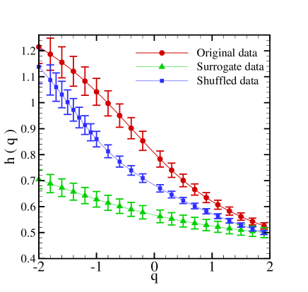
FIG. 8.: Generalized Hurst exponent, $h(q)$ as a function of $q$ for original, surrogate and shuffled data.

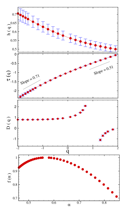
FIG. 9.: The $q$ dependence of the generalized Hurst exponent $h(q)$, the corresponding $\tau(q)$, generalized multifractal dimension $D(q)$ and singularity spectrum $f(\alpha)$ are shown in the upper to lower panel respectively for surrogate duct water of Daugava river series without sinusoidal trend.

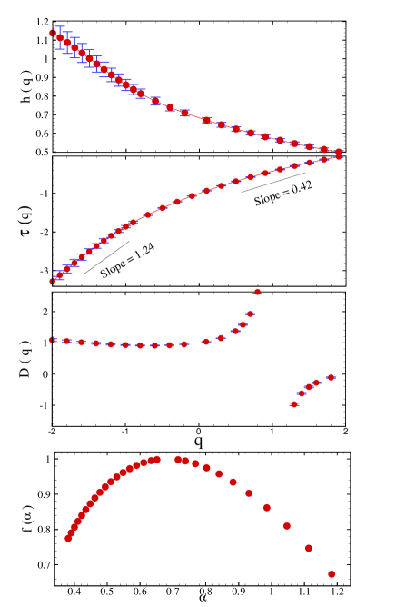
FIG. 10.: The $q$ dependence of the generalized Hurst exponent $h(q)$, the corresponding $\tau(q)$, generalized multifractal dimension $D(q)$ and singularity spectrum $f(\alpha)$ are shown in the upper to lower panel respectively for shuffled duct water of Daugava river series without sinusoidal trend.

The values of the generalized Hurst exponent $h(q=2.0)$, multifractal scaling $\tau(q=2)$ and other related scaling exponents are indicated in Table I for the original, shuffled of duct water of Daugava river series obtained with MF-DFA1 method are reported in Table I. The values of the Hurst exponent obtained by MF-DFA1 and modified MF-DFA1 methods for original, surrogate and shuffled duct water of Daugava river series are given in Table II.

V Conclusion

The MF-DFA method allows us to determine the multifractal characterization of the nonstationary and stationary time series. We apply the recent method to investigate the existence of crossover on the result of MF-DFA of river flow fluctuations. The concept of MF-DFA of runoff water of rivers can be used to gain deeper insight in to the processes occurring in climate and hydrological systems. We have shown that the MF-DFA1 result of the monthly river flows (e.g. duct water of Daugava river series) has two crossover time scale $(s_{\times})$. Our results show that there exists a tendency between some runoff river and sun activity. Indeed due to the presence of both seasonal trend and the effect of sun’s period on some river flows, we see at least two crossover in the DFA result of rivers, nevertheless, it is not expected that the number of sunspots has superior effect on runoff water fluctuations. So this effect has different intensity on the rivers. These crossover time scale are due to the sinusoidal trend. To minimizing the effect of this trend, we have applied F-DFA on the river flow time series. Applying the MF-DFA1 method on truncated data, demonstrated that the monthly duct water of Daugava river series is a stationary time series with approximately random behavior. For other rivers we found long-range correlation in their statistical behaviors. The $q$ dependence of $h(q)$ and $\tau(q)$, indicated that the monthly duct water of Daugava river series has multifractal behavior. By comparing the generalized Hurst exponent of the original time series with the shuffled and surrogate one’s, we have found that multifractality due to the broadness of the probability density function has more contribution than the correlation. The value of the Hurst exponent shows that the flow of water without seasonal trend is the same as random process.

Acknowledgements We would like to thank Mr. Rahimi Tabar and Mr. Jafari for reading the manuscript and useful comments. This paper is dedicated to Mrs. Somayeh Abdollahi and my son S. Danial Movahed.

TABLE I.: The values of the Hurst $(H)$, power spectrum scaling $(\beta)$, auto-correlation scaling $(\gamma)$ exponents and multifractal scaling for original, surrogate and shuffled of monthly duct water of Daugava river series obtained by MF-DFA1.

Data	$H$	$\beta$	$\gamma$	$\tau$
Original	$0.52\pm 0.02$	$0.04\pm 0.02$	$0.96\pm 0.02$	$0.04\pm 0.02$
Surrogate	$0.51\pm 0.02$	$0.02\pm 0.02$	$0.98\pm 0.02$	$0.02\pm 0.02$
Shuffled	$0.50\pm 0.01$	$0.00$	$1.00\pm 0.02$	$0.00$

TABLE II.: The value of the Hurst exponent using MF-DFA1 and modified MF-DFA1 for the original, shuffled and surrogate of monthly duct water of Daugava river series.

Method	Original data	Surrogate	Shuffled
MF-DFA1	$0.52\pm 0.01$	$0.51\pm 0.01$	$0.50\pm 0.01$
Modified	$0.54\pm 0.02$	$0.46\pm 0.02$	$0.51\pm 0.02$

VI APPENDIX

In this appendix we derive the relation between the exponent $h(2)$ (DFA1 exponent) and Hurst exponent of a fGn signal in one dimension. We show that for such stationary signal the average sample variance (Eq. 4) for $q=2$, is proportional to $s^{h(q)}$, where $h(q=2)=H$. It is shown that the averaged sample variance $F^{2}(s)$ behaves as:

$$F^{2}(s) \equiv \frac{1}{N_{s}}\sum_{\nu=1}^{N_{s}}\left[F^{2}(s;\nu)\right],$$ (24)

$$= \left\langle\left[F^{2}(s;\nu)\right]\right\rangle_{\nu},$$ (25)

$$\equiv {\mathcal{C}_{H}}s^{2H},$$ (26)

where $F^{2}(s;\nu)$ is defined as:

$$F^{2}(s;\nu)=\frac{1}{s}\sum_{i=1}^{s}\left[Y_{\nu}(i)-y_{\nu}(i)\right]^{2},$$ (27)

and ${\mathcal{C}_{H}}$ is a function of Hurst exponent $H$. To prove the statement we note that the data $x(k)$ is a fractional Gaussian noise (fGn), the partial sums $Y(i)$ (Eq. 1) will be a fBm signal:

$$Y(i)=\sum_{k=1}^{i}x(k)-\langle x\rangle.$$ (28)

In the DFA1, the fitting function will have the expression $(y_{\nu}(i)=a_{\nu}+b_{\nu}i)$. The slope $b_{\nu}$ and intercept $a_{\nu}$ of a least-squares line $Y(i)$ for every windows $(\nu)$ are given by:

$$b_{\nu} = \frac{\sum_{i=1}^{s}Y(i)i-\frac{1}{s}\sum_{i=1}^{s}Y(i)\sum_{i=1}^{s}i}{\sum_{i=1}^{s}i^{2}-\frac{1}{s}\left[\sum_{i=1}^{s}i\right]^{2}},$$ (30)

$$\simeq\frac{\sum_{i=1}^{s}Y(i)i-\frac{s}{2}\sum_{i=1}^{s}Y(i,j)}{s^{3}/12},$$

$$a_{\nu} = \frac{1}{s}\sum_{i=1}^{s}Y(i)-\frac{b_{\nu}}{s}\sum_{i=1}^{s}i,$$ (32)

$$\simeq\frac{1}{s}\sum_{i=1}^{s}Y(i)-\frac{b_{\nu}s}{2},$$

respectively.

Using the Eqs. 4 and 32, the Eq. 27 can be written as follows:

$$\left\langle\left[F^{2}(s;\nu)\right]\right\rangle=\left\langle\frac{1}{s}\sum_{i=1}^{s}[Y(i)-a-bi]^{2}\right\rangle,$$ (33)

$$\simeq \left\langle\frac{1}{s}\sum_{i=1}^{s}Y(i)^{2}\right\rangle+\left\langle a^{2}\right\rangle+\frac{s^{2}}{3}\left\langle b^{2}\right\rangle+s\left\langle ab\right\rangle$$ (35)

$$-2\left\langle\frac{a}{s}\sum_{i=1}^{s}Y(i)\right\rangle-2\left\langle\frac{b}{s}\sum_{i=1}^{s}iY(i)\right\rangle,$$

where we have discard the subscript $\nu$ for simplicity. The fBm signals is produced by using the fGn noise as follows:

$$Y(i)=i^{H}x,$$ (36)

and

$$Y(i)-Y(k) = |i-k|^{H}x,$$ (37)

so,

$$\langle[Y(i)-Y(k)]^{2}\rangle=\sigma^{2}|i-k|^{2H},$$ (38)

where $\sigma^{2}=\left\langle x(i)^{2}\right\rangle$. The variance of fBm signal is: $\left\langle Y(i)^{2}\right\rangle=\sigma^{2}i^{2H}$[30]. Expanding the left hand side of Eq. 38, it can be easily shown that the correlation function of $Y(i)$, has the following form:

$$\left\langle Y(i)Y(k)\right\rangle = \frac{\sigma^{2}}{2}[i^{2H}+k^{2H}-|i-k|^{2H}].$$ (39)

Finally using the Eqs. 32 and 39, it can be easily shown that the Eq. 35 can be written as follows:

$$\left\langle\left[F^{2}(s;\nu)\right]\right\rangle_{\nu}={\mathcal{C}_{H}}(s)^{2H}.$$ (40)

To determine the ${\mathcal{C}_{H}}$, we have to calculate some terms such as:

$$\sum_{i,j=1}^{s}\langle iY(i)Y(j)\rangle=\frac{\sigma^{2}}{2}\sum_{i,j=1}^{s}\left(i^{2H+1}+ij^{2H}-i|i-j|^{2H}\right),$$ (41)

$$=\frac{\sigma^{2}}{2}\sum_{i,j=1}^{s}\left(i^{2H+1}+ij^{2H}\right)-\frac{\sigma^{2}}{2}\sum_{i=1}^{s}\sum_{j=1}^{i}i(i-j)^{2H}$$ (42)

$$\qquad-\frac{\sigma^{2}}{2}\sum_{i=1}^{s}\sum_{j=i}^{s}i(j-i)^{2H},$$ (43)

$$\sim\frac{\sigma^{2}}{2}\left(\frac{s^{2H+3}}{2H+2}+\frac{s^{2H+3}}{2(2H+1)}\right)$$ (44)

$$-\frac{\sigma^{2}}{2}\sum_{i=1}^{s}i^{2H+2}\left(\int_{0}^{1}(1-x)^{2H}dx-\int_{0}^{1}x(1-x)^{2H}dx\right),$$ (45)

$$=\frac{\sigma^{2}s^{2H+3}}{4}\left(\frac{2}{H+1}-\frac{1}{2H+1}\right),$$ (46)

and

$$\sum_{i,j=1}^{s}\langle Y(i)Y(j)\rangle=\frac{\sigma^{2}}{2}\sum_{i,j=1}^{s}\left(i^{2H}+j^{2H}-|i-j|^{2H}\right),$$ (47)

$$=\frac{\sigma^{2}}{2}\sum_{i,j=1}^{s}\left(i^{2H}+j^{2H}\right)-\sigma^{2}\sum_{i=1}^{s}\sum_{j=1}^{i}(i-j)^{2H},$$ (48)

$$\sim\sigma^{2}\left(\frac{s^{2H+2}}{2H+1}-\sum_{i=1}^{s}i^{2H+1}\int_{0}^{1}(1-x)^{2H}\right),$$ (49)

$$\sim\sigma^{2}s^{2H+2}\left(\frac{1}{2H+1}-\frac{1}{(2H+2)(2H+1)}\right).$$ (50)

Finally ${\mathcal{C}_{H}}$ has the following form:

$${\mathcal{C}_{H}} = \frac{\sigma^{2}}{(2H+1)}-\frac{4\sigma^{2}}{2H+2}$$ (53)

$$+3\sigma^{2}\left(\frac{2}{H+1}-\frac{1}{2H+1}\right)$$

$$\qquad-\frac{3\sigma^{2}}{(H+1)}\left(1-\frac{1}{(H+1)(2H+1)}\right).$$

Therefore the standard DFA$1$ exponent for a stationary signal is related to its Hurst exponent as $h(q=2)=H$.

REFERENCES

- [1] E. Koscielny-Bunde, A. Bunde, S. Havlin, H.E. Roman, Y. Goldreich, H.-J. Schellnhuber, Phys. Rev. Lett. 81 729 732 (1998).
- [2] S.M. Barbosa, M.J. Fernandes and M.E. Silva, Physica A 371 (2006) 725 731.
- [3] K. Fraedrich, U. Luksch, R. Blender, Phys. Rev. E 70 (2004) 037301.
- [4] V. Livina, Y. Ashkenazy, P. Braun, R. Monetti, A. Bunde and S. Havlin, Physical Review E, 67 (2003) 042101.
- [5] V. Livina et al., Physica A, 330 (2003) 283-290.
- [6] B.B. Mandelbrot, J.R. Wallis, Water Resour. Res. 5 (1969) 321.
- [7] F. Schmitt, D. La Vall e, and D. Schertzer Phys. Rev. Lett. 68 (1992) 305 308.
- [8] P. Burlando, e R. Rosso, J. Hydrol., vol. 187/1-2 (1996) 45-64, Burlando, P., A. Montanari, e R. Rosso, Meccanica, 31 (1996) 87-101, Kluwer Ac. Publ., Dordrecht, The Netherlands.
- [9] H.E. Hurst, Transact. Am. Soc. Civil Eng. 116 770 (1951).
- [10] H.E. Hurst, R.P. Black and Y.M. Simaika, 1965 Long-term storage. An experimental study (Constable, London)
- [11] J. Feder, Fractals, Plenum Press, New York, 1988.
- [12] C. Matsoukas, S. Islam, I. Rodriguez-Iturbe, J. Geophys. Res. Atmos. 105 (2000) 29 165.
- [13] Y. Tessier, S. Lovejoy, P. Hubert, D. Schertzer, S. Pecknold, J. Geophys. Res. Atmos. 101 (1996) 26 427.
- [14] G. Pandey, S. Lovejoy, D. Schertzer, J. Hydrol. 208 (1998) 62.
- [15] R.U. Murdock, J.S. Gulliver, J. Water Res. Pl-Asce. 119 (1993) 473.
- [16] C.N. Kroll, R.M. Vogel, J. Hydrol. Eng. 7 (2003) 137.
- [17] J.D. Pelletier, D.L. Turcotte, J. Hydrol. 203 (1997) (1 4) 198.
- [18] E. Koscielny-Bunde, J.W. Kantelhardt, P. Braun, A. Bunde, S. Havlin, Water Resour. Res. 2003, arXiv:physics/0305078.
- [19] J.W. Kantelhardt, D. Rybski, S.A. Zschiegner, P. Braun, E. Koscielny-Bunde, V. Livina, S. Havlin, A. Bunde, Physica A 330 (2003) doi:10.1016/j.physa.2003.08.019 [these proceedings].
- [20] A. Bunde, et al., Physica A 330 (2003) doi:10.1016/j.physa.2003.08.004 [these proceedings].
- [21] Y. Ashkenazy et al., Phys. Rev. L., 86(9) (2001) 1900-1903.
- [22] Y. Ashkenazy et al., Physica A, 323 (2003) 19-41.
- [23] N.Loboda, Geophysical Research Abstracts, 8(2006) 00797.
- [24] Hu K, Ivanov P Ch, Chen Z, Carpena P and Stanley H E, Phys. Rev. E 64 (2001) 011114.
- [25] M. Sadegh Movahed, G. R. Jafari, F. Ghasemi, S. Rahvar and M. Rahimi Tabar, J. Stat. Mech. (2006) P02003.
- [26] http://www.oma.be/KSB-ORB/SIDC/index.html
- [27] http://waterdata.usgs.gov
- [28] R. Nagarajan and R.G. Kavasseri, arXive:cond-mat/0411543.
- [29] C. V. Chianca, A. Ticona and T.J.P Penna, Physica A, 357 (2005) 447-454.
- [30] C. K. Peng, S.V. Buldyrev, S. Havlin, M. Simons, H. E. Stanley and A.L. Goldberger, Phys. Rev. E 49 (1994) 1685; S.M. Ossadnik, S.B. Buldyrev, A.L. Goldberger, S. Havlin, R.N. Mantegna, C.K. Peng, M. Simons and H.E. Stanley, Biophys. J. 67 (1994) 64.
- [31] M.S. Taqqu, V. Teverovsky and W. Willinger, Fractals 3 (1995) 785.
- [32] J.W. Kantelhardt, E. Koscielny-Bunde, H.A. Rego, S. Havlin and A. Bunde, Physica A 295 (2001) 441.
- [33] Z. Chen, P.Ch. Ivanov, K. Hu and H.E. Stanley, Phys. Rev. E, 65 (2002) 041107.
- [34] S.V. Buldyrev, A.L Goldberger, S. Havlin, R.N. Mantegna, M.E. Matsa, C.K. Peng, M. Simons and H.E. Stanley, Phys. Rev. E 51 (1995) 5084; S.V. Buldyrev, N.V. Dokholyan, A.L. Goldberger, S. Havlin, C.K. Peng, H.E. Stanley and G.M. Viswanathan, Physica A 249 (1998) 430.
- [35] P.Ch. Ivanov et. al., Europhys. Lett. 48 (1999) 594; Y. Ashkenazy et. al., Europhys. Lett. 53 (2001) 709; Y. Ashkenazy et. al., Phys. Rev. Lett. 86 (2001) 1900.
- [36] C.K. Peng, S. Havlin, H.E. Stanley and A.L. Goldberger, Chaos 5 (1995) 82.
- [37] A. Bunde, S. Havlin, J.W. Kantelhardt, T. Penzel, J.H. Peter and K. Voigt, Phys. Rev. Lett. 85 (2000) 3736.
- [38] S. Blesic, S. Milosevic, D. Stratimirovic and M. Ljubisavljevic, Physica A 268 (1999) 275; S. Bahar, J. W. Kantelhardt, A. Neiman, H.A. Rego, D.F. Russell, L. Wilkens, A. Bunde and F. Moss, Europhys. Lett. 56 (2001) 454.
- [39] J.M. Hausdorff, S.L. Mitchell, R. Firtion, C.K. Peng, M.E. Cudkowicz, J.Y. Wei and A.L. Goldberger, J. Appl. Physiology 82 (1997) 262.
- [40] E. Koscielny-Bunde, A. Bunde, S. Havlin, H.E. Roman, Y. Goldreich and H.J. Schellnhuber, Phys. Rev. Lett. 81 (1998) 729; K. Ivanova and M. Ausloos, Physica A 274 (1999) 349; P. Talkner and R.O. Weber, Phys. Rev. E 62 (2000) 150.
- [41] K. Ivanova, M. Ausloos, E. Clothiaux and T.P. Ackerman, Europhys. Lett. 52 (2000) 40.
- [42] B.D Malamud and D.L. Turcotte, J. Stat. Plan. Infer. 80 (1999) 173.
- [43] C.L. Alados and M.A. Huffman, Ethnology 106 (2000) 105.
- [44] R. N. Mantegna and H.E. Stanley, An Introduction to Econophysics (Cambridge University Press, Cambridge) (2000); Y. Liu, P. Gopikrishnan, P. Cizeau, M. Meyer, C.K. Peng and H. E. Stanley, Phys. Rev. E 60(1999) 1390; N. Vandewalle, M. Ausloos and P. Boveroux, Physica A 269 (1999) 170.
- [45] P.Ch. Ivanov et. al., Phys. Rev. E, 69(2004) 056107.
- [46] J.W. Kantelhardt, R. Berkovits, S. Havlin and A. Bunde, Physica A 266 (1999) 461; N. Vandewalle, M. Ausloos, M. Houssa, P.W. Mertens and M. Heyns, Appl. Phys. Lett. 74 (1999) 1579.
- [47] M. Sadegh Movahed, F. Ghasemi, Sohrab Rahvar, M. Reza Rahimi Tabar, arXiv:astro-ph/0602461.
- [48] J. Feder, Fractals (Plenum Press, New York) (1988).
- [49] A.L. Barabási and T. Vicsek, Phys. Rev. A 44 (1991) 2730.
- [50] H.O. Peitgen, H. Jürgens and D. Saupe, Chaos and Fractals (Springer-Verlag, New York), Appendix B (1992).
- [51] E. Bacry, J. Delour and J.F. Muzy, Phys. Rev. E 64 (2001) 026103.
- [52] J.F. Muzy, E. Bacry and A. Arneodo, Phys. Rev. Lett. 67 (1991) 3515.
- [53] U. Fano, Phys. Rev. 72 (1947) 26.
- [54] J.A. Barmes and D.W. Allan, Proc. IEEE 54 (1996) 176.
- [55] S.V. Buldyrev, A.L. Goldberger, S. Havlin, R.N. Mantegna, M.E. Matsa, C.K. Peng, M. Simons, H.E. Stanley, Phys. Rev. E 51 (1995) 5084.
- [56] Z. Chen et. al., Phys. Rev. E, 71 (2005) 011104.
- [57] Limei Xu, Plamen Ch. Ivanov, Kun Hu, Zhi Chen, Anna Carbone, and H. Eugene Stanley, Phys. Rev. E 71 (2005) 051101.
- [58] J. W. Kantelhardt, S. A. Zschiegner, Eva Koscielny-Bunde, S. Havlin, A. Bunde and H. E. Stanley, Physica A 316, 87-114 (2002). ‡‡‡Fixme: Removed the mistake in reference [58]
- [59] A. Eke, P. Herman, L. Kocsis and L.P Kozak, Physiol. Meas. 23 (2002) R1-R38.
- [60] For the maximum scale the fluctuation function is independent of , since the sum in Eq. (4) runs over only two identical segments (). For smaller scales the averaging procedure runs over several segments, and the average value will be dominated by the from the segments with small (large) fluctuations if (). Thus, for , with will be smaller than with , while both become equal for . Hence, if we assume an homogeneous scaling behavior of following Eq. (5), the slope in a log-log plot of with versus must be larger than the corresponding slope for with . Thus, for will usually be larger than for .
- [61] E. Koscielny-Bunde, H.E. Roman, A. Bunde, S. Havlin and H.J. Schellnhuber, Phil. Mag. B 77 (1998) 1331.
- [62] E. Koscielny-Bunde, A. Bunde, S. Havlin, H.E. Roman, Y. Goldreich and H.J. Schellnhuber, Phys. Rev. Lett. 81 (1998) 729.
- [63] P. Oświȩcimka, Jaroslaw Kwapien and S. Drozdz, Phys.Rev. E 74 (2006) 016103.