Application of the $J$-matrix Method to Faddeev-Merkuriev equation: beyond pseudostates.

Abstract

A version of the $J$-matrix method for solving numerically the three-body Faddeev-Merkuriev differential equations is proposed. This version allows to take into account the full spectrum of the two-body Coulomb subsystem. As a result, a discrete analog of the Lippmann-Schwinger equation is obtained which allows to interpret correctly the three-body wave function in two-body domains. The scheme is applied to calculations of the fully resolved absolute differential cross sections for the He$(e,2e)$He⁺ and He$(e,3e)$He⁺⁺ reactions at small energy and momentum transfers. The results are in good agreement with the experiment both in shape and in absolute value.

I Introduction

The few-body Coulomb problem is one of the most fundamental problems in physics and being yet to be exactly solved. In recent years, it has attracted numerous theoretical studies which involve different approaches and/or approximations. Among these is the $J$-matrix method widely used in the quantum scattering theory. It was first proposed in atomic physics JA and later on (independently) in nuclear physics FO ; SN ; RSJ . Within this approach the full Hamiltonian of the atomic system is split into two parts $H=H_{c}+V$. The operator $H_{c}$ determines the discrete basis of square-integrable functions which are used for expansion of the many-body wave function. In atomic physics, a Laguerre basis is the most widely used because it provides the three-diagonal representation of a radial part of the operator $H_{c}$, and this infinite trinomial recurrence can be solved analytically. At the same time, the short-range interaction $V$ is approached by its projection $V^{N}$ on a subspace of $N$ basic functions. Hence, the $J$-matrix method supplies the exact solution of the scattering problem on the model potential $V^{N}$. The $J$-matrix approach is proved to be an efficient and rather accurate numerical method. Formally and from the viewpoint of a numerical realization, the $J$-matrix method is similar to the R-matrix scattering theory (for an overview, see, for example, Rmtx ). It is also equivalent to the method of the so-called Coulomb-Sturm separable expansion (see, for instance, Papp and references therein).

The most important problem in a few-body Coulomb scattering theory is the description of the continuum-state wave function in terms of square-integrable functions. The method of pseudostates and its recent avatar, the convergent close-coupling method (CCC) BS , replace the continuous energy spectrum of a selected two-body subsystem by a finite number of positive energy lines. However, we present here a new scheme which allows to take into account both the summation and integration over respectively the bound and continuum states of the two-body subsystem.

The general idea guiding the $J$-matrix method was first formulated in KS for a system of three nuclear particles interacting with short-range potentials using an oscillator basis. Recently, on a base of the results of Papp et al. PHHKY it was extended for the case of long-range Coulomb potentials ZKP . We solve the Faddeev-Merkuriev differential equations which allow to formulate the boundary conditions for a component $\psi_{\alpha}$ of the full wave function $\Psi=\sum_{\alpha}\psi_{\alpha}$ in terms of the fixed number of Jacobi coordinates ${\bf x}_{\alpha},{\bf y}_{\alpha}$. We use the fact MFB that in the two-body domain $\Omega_{\alpha}$, where the mutual distance ${\bf x}_{\alpha}$ between particles $\beta$ and $\gamma$ is much smaller than the distance ${\bf y}_{\alpha}$ between their center-of-mass and particle $\alpha$, the total asymptotic Hamiltonian $H_{as}$ looks like a direct sum of uncoupled Hamiltonians $h_{x_{\alpha}}$ and $h_{y_{\alpha}}$. As a result, the full three-body Green’s function $G=(E-H+i0)$ is connected with the asymptotic operator $G_{\alpha}=(E-h_{x_{\alpha}}-h_{y_{\alpha}}+i0)$ in the domain $\Omega_{\alpha}$. In turn, the Green’s function $G_{\alpha}$ is presented as an overlapping integral of the operators $G_{x_{\alpha}}$ and $G_{y_{\alpha}}$.

Furthermore, following Ref. ZKP the component $\psi_{\alpha}$ is presented as a decomposition on the eigenfunctions of the two-body subsystem $(\beta\gamma)$ with the total charge $Z_{\alpha}$. Such a choice allows to factor out the long-range part of the interaction and, consequently, to describe correctly the asymptotic behavior of the function $\Psi$ only in the two-body domain $\Omega_{\alpha}$. In this way, we arrive at a discrete analog of the Lippmann-Schwinger equation for the component $\psi_{\alpha}$ in $\Omega_{\alpha}$. This is the general scheme of the method, and the details are presented below.

The present paper is organized as follows. A detailed theoretical formulation of the above general scheme is presented in Section II. In Section III, the efficiency of the presented numerical scheme is demonstrated in a light of comparison with experimental data. We calculate for a helium target the $(e,2e)$ triple differential cross section (TDCS) for single ionization accompanied with simultaneous excitation, and the $(e,3e)$ five-fold differential cross section (5DCS) for double ionization under fast electron impact. Previous calculations of the three-body wave function of the system $(e,e,$He${}^{++})$ were carried out within the method of pseudostates KBLDT ; KNP as well as using other methods, such as the so-called 3C JM ; AMC , approximate 6C JM ; 6C , and C4FS C4FS . Most of theoretical results exhibited a marked disagreement with the experimental data on absolute scale KBLDT ; KNP . In this work we show that the proposed method is able to describe the same experiments without any scaling factors.

II Theory

The Hamiltonian of a three-body system has the form

$$H=H_{0}+\sum\limits_{\alpha=1}^{3}V^{C}_{\alpha}(x_{\alpha}),$$ (1)

where $H_{0}$ is the kinetic energy operator

$$H_{0}=-\triangle_{x_{\alpha}}-\triangle_{y_{\alpha}},$$ (2)

and

$$V^{C}_{\alpha}(x_{\alpha})=\frac{Z_{\alpha}}{x_{\alpha}}.$$ (3)

The couple (${\bf x}_{\alpha}$, ${\bf y}_{\alpha}$) stands for the set of Jacobi coordinates MFB

$$\begin{array}[]{c}{\bf x}_{\alpha}=\tau_{\alpha}({\bf r}_{\beta}-{\bf r}_{\gamma}),\\[8.53581pt] {\bf y}_{\alpha}=\mu_{\alpha}\left({\bf r}_{\alpha}-\frac{m_{\beta}{\bf r}_{\beta}+m_{\gamma}{\bf r}_{\gamma}}{m_{\beta}+m_{\gamma}}\right)\ ,\\ \end{array}$$ (4)

where $m_{i}$ are the particle masses and

$$\tau_{\alpha}=\sqrt{2\frac{m_{\beta}m_{\gamma}}{m_{\beta}+m_{\gamma}}},\quad\mu_{\alpha}=\sqrt{2m_{\alpha}\left(1-\frac{m_{\alpha}}{m_{1}+m_{2}+m_{3}}\right)}.$$ (5)

The interaction $V_{\alpha}$ can be decomposed into the short- and long-range parts ($V_{\alpha}^{(s)}$ and $V_{\alpha}^{(l)}$, respectively) MFB

$$V_{\alpha}^{(s)}(x_{\alpha},\,y_{\alpha})=V_{\alpha}(x_{\alpha})\zeta_{\alpha}(x_{\alpha},\,y_{\alpha}),\qquad V_{\alpha}^{(l)}(x_{\alpha},\,y_{\alpha})=V_{\alpha}(x_{\alpha})[1-\zeta_{\alpha}(x_{\alpha},\,y_{\alpha})]$$ (6)

with the ”separation” function of the form KWH

$$\zeta(x_{\alpha},y_{\alpha})=2/\left\{1+\exp[(x_{\alpha}/x_{0})^{\nu}/(1+y_{\alpha}/y_{0})]\right\}$$ (7)

where $\nu>2$. Thus, the function $V_{\alpha}^{(s)}$ decreases rather rapidly in the ”true” three-body asymptotic domain $\Omega_{0}$ and coincides with the initial potential in the two-body asymptotic domain $\Omega_{\alpha}$ ($x_{\alpha}\ll y_{\alpha}$). In the general case of different particles, the total wave function is represented as the sum of three components $\psi_{\alpha}$ satisfying the set of equations MFB

$$\left[H_{0}+V_{\alpha}(x_{\alpha})+V_{\beta}^{(l)}(x_{\beta})+V_{\gamma}^{(l)}(x_{\gamma})-E\right]\psi_{\alpha}=-V_{\alpha}^{(s)}\left(\psi_{\beta}+\psi_{\gamma}\right).$$ (8)

For the system $(e,e,{He}^{++})$ particles 1 and 2 (electrons) are identical, and the solution reduces to the sum of two components $\psi_{1}$ and $\psi_{2}$ (see, for instance, KWH ). They are related to each other as follows: $\psi_{2}=gP_{12}\psi_{1}$ ($g=+1$ and $g=-1$ for, respectively, singlet and triplet spin states, $P_{12}$ is the permutation operator). Taking into account the spatial symmetry of the total wave function, Eq. (8) can be reduced to a single equation KWH

$$[H_{0}+V_{1}(x_{1})+V_{3}(x_{3})+V_{2}^{(l)}(x_{2})-E]\psi_{1}({\bf x}_{1},\,{\bf y}_{1})=-gV_{1}^{(s)}P_{12}\psi_{1}({\bf x}_{1},\,{\bf y}_{1})$$ (9)

for the component $\psi_{1}$.

The wave function $\Psi^{(-)}$ of the system $(e,e,$He${}^{++})$ with all three particles being free can be represented by the following decomposition

$$\Psi^{(-)}=\frac{2}{\pi}\frac{1}{p_{0}\,k_{0}}\,\frac{(1+gP_{12})}{\sqrt{2}}\,\sum\limits_{\begin{subarray}{c}L\,\ell_{0}\,\lambda_{0}\\ m_{0}\,\mu_{0}\end{subarray}}(\ell_{0}\,m_{0}\,\lambda_{0}\,\mu_{0}|L\,M){i}^{\ell_{0}+\lambda_{0}}\,e^{-{i}(\sigma_{\ell_{0}}+\sigma_{\lambda_{0}})}Y_{\ell_{0}\,m_{0}}^{*}(\widehat{k}_{0})Y_{\lambda_{0}\,\mu_{0}}^{*}(\widehat{p}_{0})\,\psi^{L\,M}_{\ell_{0}\,\lambda_{0}}.\\$$ (10)

The corresponding decomposition of the function $\Psi^{(-)}_{n_{0}\ell_{0}m}$ of the system $(e,$He⁺) with two bound particles is given by

$$\Psi^{(-)}_{n_{0}\,\ell_{0}\,m}=\sqrt{\frac{2}{\pi}}\frac{1}{p_{0}}\,\frac{(1+gP_{12})}{\sqrt{2}}\,\sum\limits_{\ L\,\lambda_{0}\,\mu_{0}}(\ell_{0}\,m\,\lambda_{0}\,\mu_{0}|L\,M)\,{i}^{\lambda_{0}}\,e^{-{i}\sigma_{\lambda_{0}}}\,Y_{\lambda_{0}\,\mu_{0}}^{*}(\widehat{p}_{0})\,\psi^{L\,M}_{\ell_{0}\,\lambda_{0}},$$ (11)

where the quantum numbers $(n_{0}\,\ell_{0}\,m)$ describe the state of the He⁺ ion.

The spatial part $\psi^{L\,M}_{\ell_{0}\,\lambda_{0}}$ of the component $\psi_{1}$ in (10) and (11) can be presented in the form of a bispherical expansion

$$\psi^{L\,M}_{\ell_{0}\,\lambda_{0}}({\bf x},\,{\bf y})=\sum\limits_{\ell\;\lambda}\frac{\psi^{L}_{\ell_{0}\,\lambda_{0},\;\ell\,\lambda}(x,\,y)}{xy}\mathcal{Y}_{\ell\,\lambda}^{LM}(\widehat{x},\,\widehat{y}),\quad{\bf x}\equiv{\bf x}_{1},\quad{\bf y}\equiv{\bf y}_{1},$$ (12)

$$\mathcal{Y}_{\ell\,\lambda}^{LM}(\widehat{x},\,\widehat{y})=\sum\limits_{m\,\mu}(\ell\,m\,\lambda\,\mu|L\,M)\,Y_{\ell\,m}(\widehat{x})\,Y_{\lambda\,\mu}(\widehat{y}).\$$ (13)

In turn, and in accord with KS , we look for the radial functions $\psi^{L}_{\ell_{0}\,\lambda_{0},\;\ell\,\lambda}(x,\,y)$ in the form of an expansion

$$\psi^{L}_{\ell_{0}\,\lambda_{0},\;\ell\,\lambda}(x,\,y)=\sum\limits_{\nu}\int dka_{\nu}^{\ell\,\lambda}(k)\varphi_{k,\ell}(x)\phi_{\nu}^{\lambda}(y)$$ (14)

in the eigenfunctions $\varphi_{k,\ell}(x)$ of the Hamiltonian

$$h_{x}=-\triangle_{x}+\frac{Z_{1}}{x}$$ (15)

describing the subsystem $(2,\,3)$. Note that here we pave the way for nondemocratic successive ejection of electrons from the atom.

In (14) and hereafter $\int dk$ means the summation over the discrete states and integration over the continuous states of the subsystem $(2,\,3)$, i.e.

$$\int dka_{\nu}^{\ell\,\lambda}(k)\varphi_{k,\ell}(x)=\sum\limits_{j}\varphi_{\ell}^{(j)}(x)\,a_{\nu}^{\ell\,\lambda}({i}\kappa_{j})+\frac{2}{\pi}\int\limits_{0}^{\infty}dk\,\varphi_{\ell}(k,\,x)\,a_{\nu}^{\ell\,\lambda}(k),$$ (16)

with $\varphi^{(j)}_{\ell}$ and $\varphi_{\ell}(k,\,x)$ being the corresponding eigenfunctions of the Hamiltonian (15) [see Eqs. (41) and (42) of Appendix]. The Laguerre basis functions $\phi_{\nu}^{\lambda}$ JA are used in (14)

$$\phi_{\nu}^{\lambda}(r)=\left[(\nu+1)_{(2\lambda+1)}\right]^{-1/2}(2ur)^{\lambda+1}e^{-ur}L_{\nu}^{2\lambda+1}(2ur),$$ (17)

with $u$ being the basis parameter which suitable choice affects the rate of convergence of the numerical results.

The functions $\varphi^{(j)}_{\ell}$ and $\varphi_{\ell}(k,\,x)$ can be also decomposed on the basis functions $\phi_{n}^{\ell}$ (17). We use the analytical expressions for the coefficients $\mathcal{S}_{n\,\ell}^{(j)}$ and $\mathcal{S}_{n\ell}(k)$ of such a decomposition [see Eqs. (44) and (45) of Appendix]. Thus, the function $\psi^{L\,M}_{\ell_{0}\,\lambda_{0}}$ reads

$$\psi^{L\,M}_{\ell_{0}\,\lambda_{0}}=\sum\limits_{\ell,\,\lambda,\,n,\,\nu}C_{n\,\nu}^{L\,(\ell\,\lambda)}(E)\,\left|n\,\ell\,\nu\,\lambda;\;LM\right>,$$ (18)

$$\left|n\,\ell\,\nu\,\lambda;\;LM\right>=\frac{\phi_{n}^{\ell}(x)\,\phi_{\nu}^{\lambda}(y)}{xy}\,\mathcal{Y}^{LM}_{\ell\,\lambda}(\widehat{x},\,\widehat{y}).$$ (19)

The coefficients $C_{n\,\nu}^{L\,(\ell\,\lambda)}$ are of the form

$$C_{n\,\nu}^{L\,(\ell\,\lambda)}(E)=\int dk\,\mathcal{S}_{n\ell}(k)\,a_{\nu}^{\ell\,\lambda}(k).$$ (20)

The set of algebraic equations for the coefficients $a_{\nu}^{\ell\,\lambda}(k)$ was obtained in the papers KS ; ZKP . As a result, Eq. (9) transforms to the form

$$\mathcal{J}_{\nu\,\nu^{\prime\prime}}^{\lambda}(p)\,a_{\nu^{\prime\prime}}^{\ell\,\lambda}(k)=-\sum\limits_{\begin{subarray}{c}n,\,n^{\prime},\,\nu^{\prime}\\ \ell^{\prime},\,\lambda^{\prime}\end{subarray}}\mathcal{S}_{n\,\ell}(k)\,V^{L(\ell\,\lambda)(\ell^{\prime}\,\lambda^{\prime})}_{n\,\nu,\;n^{\prime}\,\nu^{\prime}}\,C_{n^{\prime}\,\nu^{\prime}}^{L\,(\ell^{\prime}\,\lambda^{\prime})}(E),\quad k^{2}+p^{2}=E.$$ (21)

Here $\mathcal{J}_{\nu\,\nu^{\prime}}^{\lambda}$ are the elements of the $J$-matrix [see Eq. (48) of Appendix] corresponding to the operator $(h_{y}-p^{2})$ ($h_{y}=-\triangle_{y}+{Z_{11}}/{y}$). The potential ${Z_{11}}/{y}$ describes the Coulomb interaction of the particle 1 with the center-of-mass of the subsystem $(2,\,3)$, and values $V^{L(\ell\,\lambda)(\ell^{\prime}\,\lambda^{\prime})}_{n\,\nu,\;n^{\prime}\,\nu^{\prime}}$ denote the matrix elements of the operator

$$V({\bf x},{\bf y})=V_{3}(x_{3})+V_{2}^{(l)}(x_{2})-\frac{Z_{11}}{y}+gV_{1}^{(s)}P_{12},$$ (22)

i.e.

$$V^{L(\ell\,\lambda)(\ell^{\prime}\,\lambda^{\prime})}_{n\,\nu,\;n^{\prime}\,\nu^{\prime}}=\left<n\,\ell\,\nu\,\lambda;\;LM\right|V({\bf x},\,{\bf y})\left|n^{\prime}\,\ell^{\prime}\,\nu^{\prime}\,\lambda^{\prime};\;LM\right>.$$ (23)

Within the two-body domain where $x<<y\rightarrow\infty$, the potential $V({\bf x},{\bf y})$ is a short-range one. This circumstance allows to take into account only a finite number of terms in the r.h.s. of Eq. (21). This means that $V^{L(\ell\,\lambda)(\ell^{\prime}\,\lambda^{\prime})}_{n\,\nu,\;n^{\prime}\,\nu^{\prime}}=0$ if at least one of the indexes $\{n,\,\nu,\,n^{\prime},\,\nu^{\prime}\}$ extends to some rather large number $N$. Thus, if $\nu\geq N$ then the r.h.s. of eq. (21) turns to zero, and the coefficients $a_{\nu}^{\ell\,\lambda}$ satisfy the ”free” equation

$$\mathcal{J}_{\nu\,\nu-1}^{\lambda}(p)\,a_{\nu-1}^{\ell\,\lambda}(k)+\mathcal{J}_{\nu\,\nu}^{\lambda}(p)\,a_{\nu}^{\ell\,\lambda}(k)+\mathcal{J}_{\nu\,\nu+1}^{\lambda}(p)\,a_{\nu+1}^{\ell\,\lambda}(k)=0.$$ (24)

Now we use the expression Heller

$$\mathcal{G}_{\nu\,\nu^{\prime}}^{\lambda(\pm)}(p)=-\frac{1}{p}\,\mathcal{S}_{\nu_{<}\,\lambda}(p)\,\mathcal{C}_{\nu_{>}\,\lambda}^{(\pm)}(p),\quad\nu_{<}=\min\left\{\nu,\,\nu^{\prime}\right\},\;\nu_{>}=\max\left\{\nu,\,\nu^{\prime}\right\},\\$$ (25)

for the matrix elements $\left[\mathcal{G}^{\lambda(\pm)}(p)\right]$ of the radial Green’s function. The functions $\mathcal{C}_{\nu\,\lambda}^{(\pm)}(p)$ are determined by Eq. (53) of Appendix. Since the infinite matrix $\left[\mathcal{G}^{\lambda(\pm)}(p)\right]$ formally is the inverse matrix to the infinite $J$-matrix $\left[\mathcal{J}^{\lambda}(p)\right]$ Heller , i.e.

$$-\left[\mathcal{G}^{\lambda(\pm)}(p)\right]\,\left[\mathcal{J}^{\lambda}(p)\right]=1,$$ (26)

the set of equations (21) can be rewritten in the following form

$$\begin{array}[]{l}a_{\nu}^{\ell\,\lambda}(k)=\mathcal{S}_{\nu\,\lambda_{0}}(p_{0})\delta_{(\ell\,\lambda)\,(\ell_{0}\,\lambda_{0})}\delta(k-k_{0})+\\[8.53581pt] \qquad\qquad+\sum\limits_{\begin{subarray}{c}n^{\prime},\,\nu^{\prime},\,n^{\prime\prime},\,\nu^{\prime\prime}\\ \ell^{\prime\prime},\,\lambda^{\prime\prime}\end{subarray}}\mathcal{G}_{\nu\,\nu^{\prime}}^{\lambda(-)}(p)\mathcal{S}_{n^{\prime}\,\ell}(k)\,V^{L(\ell\,\lambda)(\ell^{\prime\prime}\,\lambda^{\prime\prime})}_{n^{\prime}\,\nu^{\prime},\;n^{\prime\prime}\,\nu^{\prime\prime}}\,C_{n^{\prime\prime}\,\nu^{\prime\prime}}^{L\,(\ell^{\prime\prime}\,\lambda^{\prime\prime})}(E),\quad\nu=0,\,1,\ldots.\\ \end{array}$$ (27)

Inserting (27) into (20) and taking into account the boundary conditions for the functions $\Psi^{(-)}$ (10) and $\Psi^{(-)}_{n_{0}\,\ell_{0}\,m}$ (11), we obtain the set of equations for the expansion coefficients $C_{n\,\nu}^{L\,(\ell\,\lambda)}$ in (18). In the case, where all particles are asymptotically free, it takes the form

$$\begin{array}[]{c}C_{n\,\nu}^{L\,(\ell\,\lambda)}(E)=\delta_{(\ell\,\lambda)\,(\ell_{0}\,\lambda_{0})}\,\mathcal{S}_{n\ell_{0}}(k_{0})\,\mathcal{S}_{\nu\lambda_{0}}(p_{0})+\\[14.22636pt] \qquad\qquad+\sum\limits_{\begin{subarray}{c}n^{\prime},\,\nu^{\prime},\,n^{\prime\prime},\,\nu^{\prime\prime}\\ \ell^{\prime\prime},\,\lambda^{\prime\prime}\end{subarray}}\left[\int dk\,\mathcal{S}_{n\ell}(k)\,\mathcal{S}_{n^{\prime}\,\ell}(k)\,\mathcal{G}^{\lambda(-)}_{\nu\,\nu^{\prime}}(p)\right]\,V^{L(\ell\,\lambda)(\ell^{\prime\prime}\,\lambda^{\prime\prime})}_{n^{\prime}\,\nu^{\prime},\;n^{\prime\prime}\,\nu^{\prime\prime}}\,C_{n^{\prime\prime}\,\nu^{\prime\prime}}^{L\,(\ell^{\prime\prime}\,\lambda^{\prime\prime})}(E)\\ \end{array}$$ (28)

In the case of two asymptotically bound particles the set of equations takes the form

$$\begin{array}[]{c}C_{n\,\nu}^{L\,(\ell\,\lambda)}(E)=\delta_{(\ell\,\lambda)\,(\ell_{0}\,\lambda_{0})}\,\mathcal{S}_{n\ell_{0}}^{(n_{0})}\,\mathcal{S}_{\nu\lambda_{0}}(p_{0})+\\[14.22636pt] \qquad\qquad+\sum\limits_{\begin{subarray}{c}n^{\prime},\,\nu^{\prime},\,n^{\prime\prime}\,\nu^{\prime\prime}\\ \ell^{\prime\prime},\,\lambda^{\prime\prime}\end{subarray}}\left[\int dk\,\mathcal{S}_{n\ell}(k)\,\mathcal{S}_{n^{\prime}\,\ell}(k)\,\mathcal{G}^{\lambda(-)}_{\nu\,\nu^{\prime}}(p)\right]\,V^{L(\ell\,\lambda)(\ell^{\prime\prime}\,\lambda^{\prime\prime})}_{n^{\prime}\,\nu^{\prime},\;n^{\prime\prime}\,\nu^{\prime\prime}}\,C_{n^{\prime\prime}\,\nu^{\prime\prime}}^{L\,(\ell^{\prime\prime}\,\lambda^{\prime\prime})}(E)\\ \end{array}$$ (29)

The set of equations (28) and (29) is in fact the discrete analog of an integral equation of the Lippmann-Schwinger type, which was obtained in PHHKY . It is easy to see that the integral in square brackets of (28) coincides with the matrix elements $G_{n\,n^{\prime};\;\nu\,\nu^{\prime}}^{\ell\,\lambda\,(-)}$ of the asymptotic three-body Green’s function $\widetilde{G}^{(-)}$ in the two-body domain. It has the form of a contour overlap integral of the two-body Green’s functions $G^{(-)}_{x}$ and $G^{(-)}_{y}$ MFB

$$\widetilde{G}^{(-)}(E)=\frac{1}{2\pi{i}}\oint\limits_{\mathcal{C}}d\mathcal{E}\,G_{x}^{(-)}(\mathcal{E})G_{y}^{(-)}(E-\mathcal{E}).$$ (30)

Here the contour $\mathcal{C}$ surrounds the spectrum of the operator $h_{x}$ in a anticlockwise direction.

The integrals in the r.h.s. of Eq. (28) can be calculated directly. Note that the integrand has the following poles at the points $k_{j}=\sqrt{E+\eta^{2}_{j}}$ ($\eta_{j}={-Z_{11}}/[{2(\lambda+j+1)}]$) which correspond to the discrete spectrum of the Hamiltonian $h_{y}$ and have a densening point at $k_{\infty}=\sqrt{E}$. The presence of the matrix element of the radial Green’s function $\mathcal{G}^{\lambda(-)}_{\nu\,\nu^{\prime}}(p)$ in the integrand means that the poles have to be rounded in a clockwise direction (Fig. 1).

Let us note that the poles can be allocated more uniformly along the contour of integration if one carries out the transformation of variable. For example, if one puts $q={-Z_{11}}/(2\sqrt{k^{2}-E})$ then the poles are disposed at the points $q_{j}=\lambda+1+j$. Thus, the integral under consideration can be performed as an infinite sum of integrals $I_{j}$ along segments $L_{j}$, in which the poles are localized, and integral $I_{e}$ with a smooth integrand, which is calculated along the segment $L_{e}$ disposing to the right of the segment $L_{0}$. Using the Sokhotsky formula we obtain

$$\begin{array}[]{c}I_{j}=\frac{2}{\pi}\,\hbox to0.0pt{$\displaystyle-$\hss}{\int\limits_{L_{j}}}dk\mathcal{S}_{n\ell}(k)\,\mathcal{S}_{n^{\prime}\,\ell}(k)\,\mathcal{G}^{\lambda(-)}_{\nu\,\nu^{\prime}}(p)-2{i}\,\mathcal{S}_{n\ell}(k_{j})\mathcal{S}_{n^{\prime}\,\ell}(k_{j})\mathop{Res}\limits_{k=k_{j}}\mathcal{G}^{\lambda(-)}_{\nu\,\nu^{\prime}}(p)=\\[8.53581pt] \qquad\qquad\qquad=\frac{2}{\pi}\,\hbox to0.0pt{$\displaystyle-$\hss}{\int\limits_{L_{j}}}dk\mathcal{S}_{n\ell}(k)\,\mathcal{S}_{n^{\prime}\,\ell}(k)\,\mathcal{G}^{\lambda(-)}_{\nu\,\nu^{\prime}}(p)+\frac{{i}}{k_{j}}\mathcal{S}_{n\ell}(k_{j})\mathcal{S}_{n^{\prime}\,\ell}(k_{j})\,\mathcal{S}_{\nu\,\lambda}^{(j)}\,\mathcal{S}_{\nu^{\prime}\,\lambda}^{(j)}.\\ \end{array}$$ (31)

For $E<0$ the matrix elements $G_{n\,n^{\prime};\;\nu\,\nu^{\prime}}^{\ell\,\lambda\,(-)}$ can be calculated without difficulties because the number of poles is finite and (usually) not numerous. For $E>0$ we must calculate an infinite number of integrals in (31). In this particular case we calculate the overlap integral (30) being written now for the matrix elements

$$G_{n\,n^{\prime};\;\nu\,\nu^{\prime}}^{\ell\,\lambda\,(-)}(E)=\frac{1}{2\pi{i}}\int\limits_{\mathcal{C}}d\mathcal{E}\,\mathcal{G}^{\ell\,(-)}_{n\,n^{\prime}}(\sqrt{\mathcal{E}_{0}+\mathcal{E}})\mathcal{G}^{\lambda(-)}_{\nu\,\nu^{\prime}}(\sqrt{\mathcal{E}_{0}-\mathcal{E}}),$$ (32)

with $\mathcal{E}_{0}=\frac{1}{2}E$, and use the method of Shakeshaft RS . The poles and cuts of the integrand in (32) are shown in Fig. 2 (here $\varepsilon$ is not infinitesimal for visualization) . To simplify calculations we rotate the contour $\mathcal{C}$ by a positive angle $\varphi$, and the new contour $\mathcal{C}^{\prime}=\mathcal{E}_{0}e^{i\varphi}t$ is depicted by the dotted line.

The integral (32) is calculated numerically along the contour $\mathcal{C}^{\prime}$. To explain details of integration we subdivide the path of integration conventionally into two parts: $\mathcal{C}^{\prime}_{1}\ (t<0)$ and $\mathcal{C}^{\prime}_{2}\ (t>0)$. We also introduce for brevity two variables: $p=\sqrt{\mathcal{E}_{0}-\mathcal{E}}$ and $k=\sqrt{\mathcal{E}_{0}+\mathcal{E}}$. Note that $\arg(p)>0$ for $t<0$, whereas $\mathcal{C}_{\nu\,\lambda}^{(-)}(p)$ and $\mathcal{G}_{\nu\,\nu^{\prime}}^{\lambda(-)}(p)$ are defined at $-\pi<\arg(p)<0$. To define $\mathcal{G}_{\nu\,\nu^{\prime}}^{\lambda(-)}(p)$ on $\mathcal{C}^{\prime}_{1}$ we use the analytic continuation Broad $\mathcal{C}_{\nu\,\lambda}^{(-)}(p)=\mathcal{C}_{\nu\,\lambda}^{(+)}(p)-2{i}\mathcal{S}_{\nu\,\lambda}(p)$, or

$$\mathcal{G}_{\nu\,\nu^{\prime}}^{\lambda(-)}(p)=\mathcal{G}_{\nu\,\nu^{\prime}}^{\lambda(+)}(p)+\frac{2{i}}{p}\mathcal{S}_{\nu\,\lambda}(p)\,\mathcal{S}_{\nu^{\prime}\,\lambda}(p).$$ (33)

At the same time, the contour $\mathcal{C}^{\prime}_{1}$ passes in the domain of definition of the function $\mathcal{G}^{\ell\,(-)}_{n\,n^{\prime}}(k)$.

Reasoning by analogy allows us to integrate along the contour $\mathcal{C}^{\prime}_{2}$. Finally we obtain in the limit $\varepsilon\to 0$

$$\begin{array}[]{c}G_{n\,n^{\prime};\;\nu\,\nu^{\prime}}^{\ell\,\lambda\,(-)}(E)=\frac{\displaystyle\mathcal{E}_{0}e^{{i}\varphi}}{\displaystyle 2\pi{i}}\left\{\int\limits_{-\infty}^{0}dt\,\mathcal{G}^{\ell\,(-)}_{n\,n^{\prime}}(k)\left[\mathcal{G}^{\lambda(+)}_{\nu\,\nu^{\prime}}(p)+\frac{2{i}}{p}\mathcal{S}_{\nu\,\lambda}(p)\,\mathcal{S}_{\nu^{\prime}\,\lambda}(p)\right]\right.+\\[8.53581pt] \qquad\qquad\qquad\qquad\qquad+\left.\int\limits_{0}^{\infty}dt\left[\mathcal{G}_{n,n^{\prime}}^{\ell(+)}(k)+\frac{2{i}}{k}\mathcal{S}_{n\,\ell}(k)\,\mathcal{S}_{n^{\prime}\,\ell}(k)\right]\mathcal{G}^{\lambda(-)}_{\nu\,\nu^{\prime}}(p)\right\}.\\ \end{array}$$ (34)

Calculating the second term in (33) we accept in accordance with Broad that

$$\left|\Gamma(\ell+1+{i}t)\right|^{2}\rightarrow\Gamma(\ell+1+{i}t)\Gamma(\ell+1-{i}t),$$ (35)

as well as calculating $\xi^{-2{i}t}$ we choose the minimal meaning of the argument $\xi$ at the range $-\pi<\arg(\xi)\leq\pi$.

III Results and discussion

To illustrate the efficiency of the presented numerical scheme, calculations of the triple differential cross section (TDCS) for $(e,2e)$ single ionization and five-fold differential cross section (5DCS) for $(e,3e)$ double-ionization reactions on the helium atom in a singlet state were performed. If a fast projectile electron of energy about several kiloelectronvolts transfers to the atom relatively small amounts of energy and momentum, the respective four-body problem can be sufficiently simplified by examining only the first Born approximation in the interaction of the projectile electron with the atom. The calculations were performed in the limit $m_{3}=\to\infty$; that is, ${\bf x}_{1}=\sqrt{2}{\bf r}_{2}$ and ${\bf y}_{1}=\sqrt{2}{\bf r}_{1}$ (atomic units are used $m_{e}=e=\hbar=1$).

The triple differential cross section (TDCS) of He$(e,2e)$He⁺ reaction when the residual He⁺ ion remains in an exited state is written in the form

$$\sigma^{(3)}_{n_{0}}\equiv\frac{d^{3}\sigma_{n_{0}}}{d\Omega_{s}dE_{1}\,d\Omega_{1}}=\sum\limits_{\ell_{0}\,m}\frac{4p_{s}k_{1}}{p_{i}Q^{4}}\left|\left<\Psi^{(-)}_{n_{0}\ell_{0}m}\right|\exp({i}{\bf Q}{\bf r}_{1})+\exp({i}{\bf Q}{\bf r}_{2})-2\left|\Psi_{0}\right>\right|^{2},$$ (36)

where $(E_{i},{\bf p}_{i})$, $(E_{s},{\bf p}_{s})$, and $(E_{1},{\bf k}_{1})$ are the energy and momentum of, respectively, the incident (fast), the scattered (fast), and the ejected (slow) electron; ${\bf Q}={\bf p}_{i}-{\bf p}_{s}$ is the transferred momentum.

The five-fold differential cross section (5DCS) of He$(e,3e)$He⁺⁺ reaction is given by

$$\sigma^{(5)}\equiv\frac{d^{5}\sigma}{d\Omega_{s}dE_{1}\,d\Omega_{1}dE_{2}\,d\Omega_{2}}=\frac{p_{s}k_{1}k_{2}}{2p_{i}Q^{4}}\left|\left<\Psi^{(-)}({\bf k}_{1},{\bf k}_{2})\right|\exp({i}{\bf Q}{\bf r}_{1})+\exp({i}{\bf Q}{\bf r}_{2})-2\left|\Psi_{0}\right>\right|^{2},$$ (37)

where $(E_{1},{\bf k}_{1})$ and $(E_{1},{\bf k}_{2})$ are the energies and momenta of both ejected slow electrons.

The final-state wave functions $\Psi^{(-)}$ (10) and $\Psi^{(-)}_{n_{0}\ell_{0}m}$ (11) are obtained using the method described in the previous Section. We have restricted ourselves to the maximum value of the total orbital angular momentum, $L_{max}=2$, and $\ell,\,\lambda\leq 3$. The number of basis functions (17) for each Jacobi coordinate $x$ and $y$ is taken as $N=21$. The basis parameter $u$ (17) affects the rate of convergence of the numerical results, and its optimum value turned out to be $u=0.3$. We also use the following parameters of the separation function (7): $\nu=2.5$; $x_{0}=0.9$; $y_{0}=6$.

The helium ground-state wave function $\Psi_{0}$ is obtained as a result of diagonalization of the matrix (1) which was calculated in the basis (19). The orthonormal functions

$$\varphi_{n}^{\ell}(r)=\left[\frac{(n+1)_{(2\ell+2)}}{2u}\right]^{-1/2}(2ur)^{\ell+1}e^{-ur}L_{n}^{2\ell+2}(2ur)$$ (38)

are used here instead of functions (17). Here we put $\ell_{max}=3$ and $n_{max}=\nu_{max}=15$. Choosing the basis parameter $u_{0}=1.193$ yields the value $E_{0}=-2.903256$ for the ground-state energy.

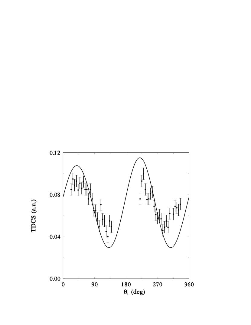
Figure 4: The same as in Fig. 3, except $E_{1}=10$ eV and $\theta_{s}=0.32^{o}$.

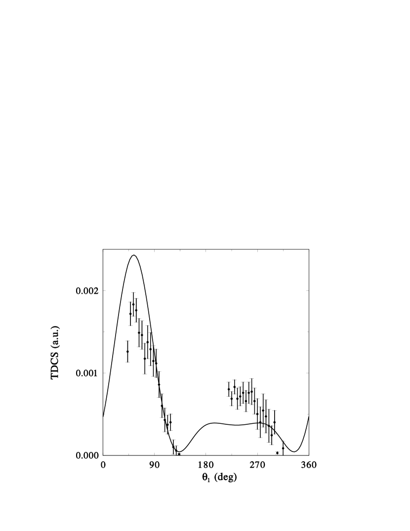
Figure 5: The same as in Fig. 3, except $E_{1}=75$ eV and $\theta_{s}=1^{o}$.

The angular distributions of the slow electron in the case of $(e,2e)$ ionization-excitation reaction are presented in Figs. 3 - 5, $\theta_{1}$ being its in-plane emission angle with respect to the vector ${\bf p}_{i}$. The displayed experimental data, which correspond to the general kinematic conditions $n_{0}=2$, $E_{s}=5500$ eV, and three particular cases $E_{1}=5$ eV and $\theta_{s}=0.35^{o}$ (Fig. 3), $E_{1}=10$ eV and $\theta_{s}=0.32^{o}$ (Fig.4), and $E_{1}=75$ eV and $\theta_{s}=1^{o}$ (Fig. 5), where $\theta_{s}$ is the scattering angle, are borrowed from DLD .

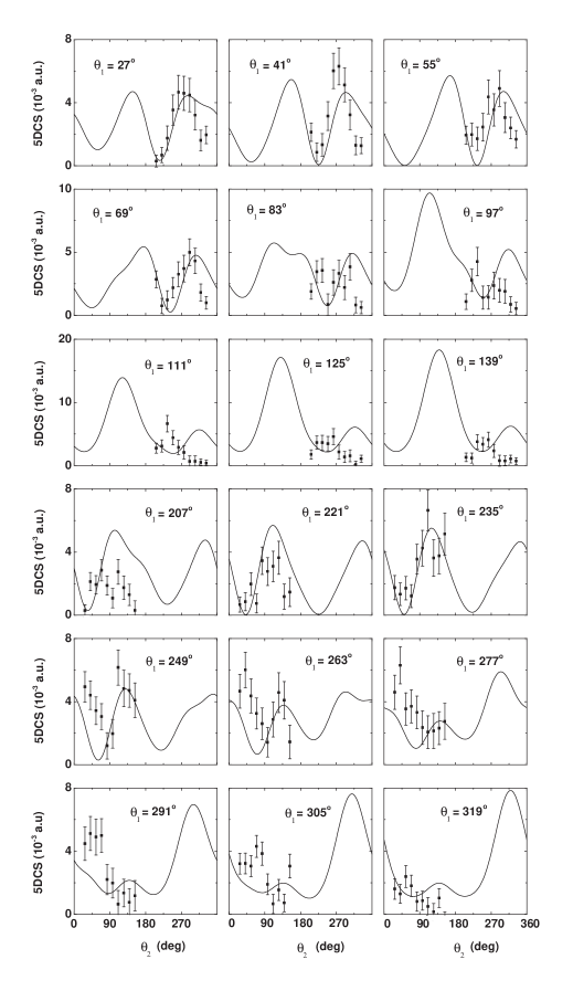
Figure 6: The fully resolved five-fold differential cross section 5DCS of the electron-impact double ionization reaction He$(e,3e){\rm He}^{++}$. The energy of the scattered electron is $E_{s}=5500$ eV, and the energies of the slow ejected electrons are $E_{1}=E_{2}=10$ eV. The scattering angle of the fast incident electron is fixed $\theta_{s}=0.45^{o}$, and the angles of the ejected electrons are $\theta_{1}$ and $\theta_{2}$, where one angle is fixed while the other angle varies relative to the incident electron direction. All electron velocities are disposed on the same plane. The absolute measurements are borrowed from C4FS .

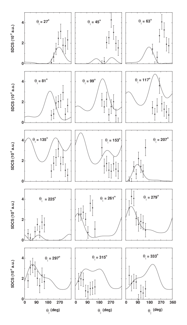
Figure 7: The same as in Fig. 6, except the ejection energies are lowered to $E_{1}=E_{2}=4$ eV.

The results for $\sigma^{(5)}$ are presented in Figs. 6 and 7. The in-plane angle $\theta_{1}$ of one of the two slow electrons is fixed, while the in-plane angle $\theta_{2}$ of the other slow electron varies. The energy of the scattered electron $E_{s}=5500$ eV and its in-plane angle $\theta_{s}=0.45^{o}$ is also fixed in all experiments. The energies of the slow electrons are $E_{1}=E_{2}=10$ eV (Fig. 6) and $E_{1}=E_{2}=4$ eV (Fig. 7). One can see that our results quite satisfactorily agree with the experimental distributions both in shape and in absolute value. This agreement in absolute scale favorably distinguishes our calculations from that obtained earlier in KBLDT ; KNP by the method of pseudostates. Considerable scaling factors were needed there to compare theory and experiment.

Let us discuss this success of our treatment in more detail. The exact final state wave function $|\Psi^{(-)}({\bf k}_{1},{\bf k}_{2})>$ must be normalized

$$<\Psi^{(-)}({\bf k}^{\prime}_{1},{\bf k}^{\prime}_{2})|\Psi^{(-)}({\bf k}_{1},{\bf k}_{2})>=\delta({\bf k}_{1}-{\bf k}^{\prime}_{1})\delta({\bf k}_{2}-{\bf k}^{\prime}_{2})+\delta({\bf k}_{1}-{\bf k}^{\prime}_{2})\delta({\bf k}_{2}-{\bf k}^{\prime}_{1})$$

The symmetrized sum of plane waves obviously possesses this property, as well as do Coulomb waves. Recent calculations with a 3C function JM ; AMC

$$\Psi^{(-)}_{3C}({\bf k}_{1},{\bf k}_{2};{\bf r}_{1},{\bf r}_{2})=\frac{(1+gP_{12})}{\sqrt{2}}\ e^{-i{\bf k}_{12}{\bf r}_{12}}\varphi_{1}^{-}({\bf k}_{1},{\bf r}_{1})\varphi_{2}^{-}({\bf k}_{2},{\bf r}_{2})\varphi_{12}^{-}({\bf k}_{12},{\bf r}_{12})$$ (39)

and some variational ground-state helium functions have demonstrated striking agreement with the experiment, although the published evidences that this function is normalized are unknown to us.

It is also obvious that the function $\Psi^{(-)}$ being decomposed into a finite sum of square-integrable functions can never be normalized to $\delta$ function. Our numerical scheme allows to conclude that the asymptotic bound of the function $\Psi^{(-)}$ is a product of two Coulomb functions in the discrete representation. Presumably, it is this property which provides much better normalization conditions for the continuum wave function than in the case of the pseudostates’ approach.

As a summary, we formulate two main conclusions

• The proposed numerical scheme and calculations demonstrate the importance of accounting for the whole two-body continuum spectrum. The method of pseudostates which replaces the continuum by a finite number of states with positive energies, seems to face with serious difficulties as to the magnitude of the calculated differential cross sections, especially when the resulting final-state wave function is applied to the calculation of $(e,3e)$ matrix elements KBLDT ; KNP .

• We observe a lack of coincidence between the theory and experiment in some kinematical cases. This, perhaps, testifies to a necessity of taking into account the correct behavior of the function $\Psi^{(-)}$ in a ”true”  three-body asymptotic region. The simple 3C model (39) partially accounts for such a behavior.

Finally we can conclude that the presented method based on the $J$-matrix approach allows to formulate the effective numerical scheme for applications in atomic physics.

*

Appendix A

The Hamiltonian

$$H_{\ell}=-\frac{d^{2}}{dr^{2}}+\ell(\ell+1)/r^{2}+{2Z}/r$$ (40)

has the following wave functions of the bound spectrum ($Z<0$)

$$\varphi^{(j)}_{\ell}(r)=(2\kappa_{j}\,r)^{\ell+1}e^{-\kappa_{j}\,r}\frac{\sqrt{-Z\,(j+1)_{2\ell+1}}}{(j+\ell+1)(2\ell+1)!}\;{{}_{1}F_{1}}(-j;\;2\ell+2;\;2\kappa_{j}\,r),$$ (41)

and continuous spectrum

$$\varphi_{\ell}(k,\,r)=\frac{1}{2}(2kr)^{\ell+1}\,e^{-\pi t/2}\,e^{{i}kr}\frac{\left|\Gamma(\ell+1+{i}t)\right|}{(2\ell+1)!}\,{{}_{1}F_{1}}(\ell+1+{i}t;\;2\ell+2;\;-2{i}kr).$$ (42)

They can be expanded in the Laguerre basis functions JA

$$\phi_{n}^{\ell}(r)=\left[(n+1)_{(2\ell+1)}\right]^{-1/2}(2ur)^{\ell+1}e^{-ur}L_{n}^{2\ell+1}(2ur)$$ (43)

and the expansion coefficients $\mathcal{S}_{n\,\ell}^{(j)}$ and $\mathcal{S}_{n\,\ell}(k)$ are given by JA ; Broad

$$\begin{array}[]{l}\mathcal{S}_{n\ell}^{(j)}=(-1)^{n}\,\left(\frac{4u\kappa_{j}}{(u+\kappa_{j})^{2}}\right)^{\ell+1}\,\left(\frac{u-\kappa_{j}}{u+\kappa_{j}}\right)^{n+j}\,\frac{\sqrt{-Z\,(j+1)_{2\ell+1}\,(n+1)_{2\ell+1}}}{(j+\ell+1)(2\ell+1)!}\,\times\\[8.53581pt] \qquad\quad\qquad\qquad\qquad\qquad\qquad\qquad\qquad\times{{}_{2}F_{1}}\left(-n,-j;\;2\ell+2;\;1-\left(\frac{u+\kappa_{j}}{u-\kappa_{j}}\right)^{2}\right)\\ \end{array}$$ (44)

and

$$\begin{array}[]{c}\mathcal{S}_{n\ell}(k)=\frac{1}{2}\,\sqrt{(n+1)_{2\ell+1}}\,(2\sin\zeta)^{\ell+1}\,e^{-\pi t/2}\,\xi^{-{i}t}\frac{\displaystyle\left|\Gamma(\ell+1+{i}t)\right|}{\displaystyle(2\ell+1)!}\,\times\\[8.53581pt] \qquad\qquad\qquad\qquad\qquad\times(-\xi)^{n}\,{{}_{2}F_{1}}\left(-n,\,\ell+1+{i}t;\;2\ell+2;\;1-\xi^{-2}\right).\\ \end{array}$$ (45)

Here $\kappa_{j}=-{Z}/{(j+\ell+1)}$, $t={Z}/{k}$, and $\xi=e^{{i}\zeta}=({{i}u-k})/({{i}u+k})$.

It is proved JA that the functions $\mathcal{S}_{n\ell}^{(j)}$, $\mathcal{S}_{n\,\ell}$ are the regular solutions of the infinite trinomial recurrence which is a discrete analog of the Schrödinger equation

$$\mathcal{J}_{n,\,n-1}^{\ell}(k)d_{n-1}+\mathcal{J}_{n,\,n}^{\ell}(k)d_{n}+\mathcal{J}_{n,\,n+1}^{\ell}(k)d_{n+1}=0\qquad(n=1,2,\ldots)$$ (46)

with the initial condition

$$\mathcal{J}_{0,\,0}^{\ell}(k)d_{0}+\mathcal{J}_{0,\,1}^{\ell}(k)d_{1}=0.$$ (47)

In (46) $\mathcal{J}_{n,\,n^{\prime}}^{\ell}(k)$ are the elements of three-diagonal matrix of the operator $(H_{\ell}-k^{2})$ (i.e. $J$-matrix) calculated with the basis functions $\phi_{n}^{\ell}$

$$\begin{array}[]{c}\mathcal{J}_{n\,n}^{\ell}(k)=\frac{u^{2}-k^{2}}{u}(n+\ell+1)+2Z,\\[8.53581pt] \mathcal{J}_{n\,n-1}^{\ell}(k)=\frac{u^{2}+k^{2}}{2u}\sqrt{n(n+2\ell+1)},\\[8.53581pt] \mathcal{J}_{n\,n+1}^{\ell}(k)=\frac{u^{2}+k^{2}}{2u}\sqrt{(n+1)(n+2\ell+2)}.\\ \end{array}$$ (48)

The coefficient functions $\mathcal{S}_{n\ell}^{(j)}$, $\mathcal{S}_{n\,\ell}$ satisfy the normalization conditions

$$\begin{array}[]{c}\sum\limits_{n,\,n^{\prime}=0}^{\infty}\mathcal{S}_{n\ell}^{(j)}\,Q_{n,\,n^{\prime}}^{\ell}\,\mathcal{S}_{n^{\prime}\ell}^{(j^{\prime})}=\delta_{j,\,j^{\prime}},\\[11.38109pt] \frac{2}{\pi}\sum\limits_{n,\,n^{\prime}=0}^{\infty}\mathcal{S}_{n\ell}(k)\,Q_{n,\,n^{\prime}}^{\ell}\,\mathcal{S}_{n^{\prime}\ell}(k^{\prime})=\delta(k-k^{\prime}),\\ \end{array}$$ (49)

where $Q_{n\,n^{\prime}}^{\ell}$ are the elements of three-diagonal matrix and are given by the overlapping integrals

$$Q_{n\,n^{\prime}}^{\ell}=\int_{0}^{\infty}\phi_{n}^{\ell}(r)\phi_{n^{\prime}}^{\ell}(r)dr,$$ (50)

$$\begin{array}[]{c}Q_{n\,n-1}^{\ell}=-\frac{\displaystyle 1}{\displaystyle 2u}\sqrt{n(n+2\ell+1)},\quad Q_{n\,n+1}^{\ell}=-\frac{\displaystyle 1}{\displaystyle 2u}\sqrt{(n+1)(n+2\ell+2)},\\[8.53581pt] Q_{n\,n}^{\ell}=\frac{\displaystyle 1}{\displaystyle u}(n+\ell+1).\\ \end{array}$$ (51)

The corresponding completeness condition takes the form

$$\frac{2}{\pi}\int\limits_{0}^{\infty}dk\,Q_{n,\,n^{\prime\prime}}^{\ell}\mathcal{S}_{n^{\prime\prime}\ell}(k)\mathcal{S}_{n^{\prime}\ell}(k)+\sum_{j=0}^{\infty}Q_{n,\,n^{\prime\prime}}^{\ell}\mathcal{S}_{n^{\prime\prime}\ell}^{(j)}\,\mathcal{S}_{n^{\prime}\ell}^{(j)}=\delta_{n\,n^{\prime}}.$$ (52)

The irregular solution of Eq. (46) can be written in the form JA ; Broad

$$\begin{array}[]{c}\mathcal{C}_{n\,\ell}^{(\pm)}(k)=-\sqrt{n!(n+2\ell+1)!}\,\frac{\displaystyle e^{\pi t/2}\xi^{{i}t}}{\displaystyle(2\sin\zeta)^{\ell}}\,\frac{\displaystyle\Gamma(\ell+1\pm{i}t)}{\displaystyle\left|\Gamma(\ell+1\pm{i}t)\right|}\times\\[8.53581pt] \qquad\qquad\qquad\qquad\times\frac{\displaystyle(-\xi)^{\pm(n+1)}}{\displaystyle\Gamma(n+\ell+2\pm{i}t)}\,{{}_{2}F_{1}}\left(-\ell\pm{i}t,\,n+1;\;n+\ell+2\pm{i}t;\;\xi^{\pm 2}\right).\\ \end{array}$$ (53)

The function $\mathcal{C}_{n\,\ell}^{(+)}(k)$ $\left(\mathcal{C}_{n\,\ell}^{(-)}(k)\right)$ is determined at ${\rm Im}({k})>0$ [${\rm Im}({k})<0$] of the complex plane $k$. The analytical continuation can be done with the help of the following relation Broad :

$$\mathcal{C}_{n\,\ell}^{(+)}(k)=\mathcal{C}_{n\,\ell}^{(-)}(k)+2{i}\mathcal{S}_{n\,\ell}(k).$$ (54)

Figure 1: The integration contour of the integral in parentheses in Eq. (28). The poles of the integrand are shown as closed circles.

Figure 2: The path of integration of the convolution integral (32). The poles which are associated with the discrete spectrum of the Hamiltonian $h_{x}$ are depicted as closed circles. $-\mathcal{E}_{0}+{i}\varepsilon$ denotes the initial point of the corresponding unitary branch cut. Open circles and $\mathcal{E}_{0}-{i}\varepsilon$ are the same for the Hamiltonian $h_{y}$.

Figure 3: TDCS for the ionization-excitation reaction He$(e,2e){\rm He}^{+}$ when the helium ion is left in the state $n_{0}=2$. The fast scattered electron energy is $E_{s}=5500$ eV, while $E_{1}=5$ eV for the slow ejected electron. The scattering angle of the fast incident electron is fixed $\theta_{s}=0.35^{o}$, and the angle of the ejected electron $\theta_{1}$ varies relative to the incident electron direction. All electron velocities are disposed on the same plane. The experimental data are borrowed from DLD .

References

• (1) E. J. Heller and H. A. Yamani, Phys. Rev. A 9, 1201 (1974); H. A. Yamani and L. Fishman, J. Math. Phys. 16, 410 (1975); J. T. Broad and W. P. Reinhardt, Phys. Rev. A 14, 2159 (1976).
• (2) G. F. Fillipov and I. P. Okhrimenko, Sov.J.Nucl.Phys 32, 480 (1980); G. F. Fillipov, Sov.J.Nucl.Phys 33, 488 (1981).
• (3) Yu. F. Smirnov and Yu. I. Nechaev, Sov.J.Nucl.Phys 35, 808 (1982).
• (4) J. Revai, M. Sotona, and J. Zofka, J. Phys. G 11, 745 (1985).
• (5) A. M. Lane and R. G. Thomas, Rev. Mod. Phys. 30, 257 (1958).
• (6) Z. Papp, Phys. Rev. C 55, 1080 (1997).
• (7) I. Bray and A. T. Stelbovics, Phys. Rev. A 46, 6995 (1992).
• (8) V. A. Knyr and L. Ya. Stotland, Sov.J.Nucl.Phys 55, 1626 (1992); Phys.At.Nucl. 56, 886 (1993); Phys.At.Nucl. 59, 575 (1996).
• (9) S. A. Zaitsev, V. A. Knyr, and Yu. V. Popov, Phys.At.Nucl. 69, 255 (2006).
• (10) Z. Papp, C-. Y. Hu, Z. T. Hlousek, B. Konya, S. L. Yakovlev, Phys. Rev. A 63, 62721 (2001).
• (11) S. P. Merkuriev and L. D. Faddeev, Quantum Scattering Theory for Several Particle Systems (Kluwer Academic Publishers, Dordrecht, 1993).
• (12) A. Kheifets, I. Bray, A. Lahmam-Bennani, et al., J. Phys. B 32, 5047 (1999).
• (13) V. A. Knyr, V. V. Nasyrov, and Yu. V. Popov, JETP 92, 789 (2001); in Correlation and Polarization in Photonic, Electronic, and Atomic Collisions, eds. G.F. Hanne, L. Malegat and H. Schmidt-Böcking, AIP Conf.Proc. 697, 76 (2003).
• (14) S. Jones and D. H. Madison, Phys. Rev. Lett. 91, 073201 (2003); S.  Jones, J. H.  Macek, and D. H.  Madison. Phys. Rev. A 70, 012712 (2004).
• (15) L. U.  Ancarani, T.  Montagnese, and C.  Dal Cappello, Phys. Rev. A 70, 012711 (2004).
• (16) A. W. Malcherek and J. S. Briggs, J. Phys. B 30, 4419 (1997); J. R. Gotz, M. Walter, and J. S. Briggs, J. Phys. B 36, L77 (2003).
• (17) A. Lahmam-Bennani, I. Taouil, A. Duguet et al., Phys.Rev.A 59, 3548 (1999).
• (18) A. A. Kvitsinsky, A. Wu, and C.-Yu  Hu, J. Phys. B 28, 275 (1995).
• (19) J. T. Broad, Phys. Rev. A, 31, 1494 (1985).
• (20) E. J. Heller, Phys. Rev. A 12, 1222 (1975).
• (21) R. Shakeshaft, Phys. Rev. A, 70, 042704 (2004).
• (22) C. Dupré, A. Lahmam-Bennani, A. Duguet et al, J. Phys. B, 25, 259 (1992).