Low frequency fluctuations in a Vertical Cavity Lasers:
experiments versus Lang-Kobayashi dynamics

Abstract

The limits of applicability of the Lang-Kobayashi (LK) model for a semiconductor laser with optical feedback are analyzed. The model equations, equipped with realistic values of the parameters, are investigated below solitary laser threshold where Low Frequency Fluctuations (LFF) are usually observed. The numerical findings are compared with experimental data obtained for the selected polarization mode from a Vertical Cavity Surface Laser (VCSEL) subject to polarization selective external feedback. The comparison reveals the bounds within which the dynamics of the LK can be considered as realistic. In particular, it clearly demonstrates that the deterministic LK, for realistic values of the linewidth enhancement factor $\alpha$, reproduces the LFF only as a transient dynamics towards one of the stationary modes with maximal gain. A reasonable reproduction of real data from VCSEL can be obtained only by considering noisy LK or alternatively deterministic LK for extremely high $\alpha$-values.

I Introduction

The dynamics of semiconductor lasers with optical feedback is studied both experimentally and theoretically since almost 30 years (primolff , for a review see e.g. book_lff ). The interest for such configuration, commonly encountered in many applications (e.g, communication in optical fibers, optical data storage, sensing etc) arises from the rich phenomenology observed, ranging from multistability, bursting, intermittency, irregular and rare drops of the intensity (low frequency fluctuations (LFF)) and transition to developed chaos (coherence collapse (CC)). A complete understanding of the physical mechanisms at the basis of such complex behavior is, however, still lacking. In particular, the origin of the LFF regime is under debate since the very first observations and yet this puzzling problem has not been solved. Their origin was ascribed to stochastic effects hk ; hohl or to deterministic but chaotic dynamics sano , and more recently even to the interplay between regular periodic and quasi-periodic solutions david . The LFF dynamics has been investigated by using several type of emitters, mainly edge-emitting: ranging from longitudinal multimode multi_exp1 ; excit ; multi_exp2 ; multi_teo1 ; multi_teo2 ; multi_teo3 ; solari to single-mode DFB dfb semiconductor lasers.

From the experimental point of view, a complete characterization of the LFF dynamics is quite difficult, because of the very different time-scales involved romanelli . Indeed, fast oscillations on the 10-ps range have been observed with streak camera measurements streak1 ; streak2 , representing the fundamental scale on which the system evolves. On the other hand, the duration of such fast pulsing regime between LFF events can be as long as hundreds of nanoseconds or even microseconds. In literature, the LFF dynamics has been experimentally characterized in several manners, starting from a relatively simple statistical analysis of the time separation T between LFFsukov ; stat1 ; dfb (relating the average $\langle T\rangle$ between LFF with the pump current) to Hurst exponents for the laser phase dynamics lam .

A widely used theoretical description of the system is the Lang-Kobayashi model LK , introduced in 1980 in the effort to provide a simplified but effective analysis of an edge-emitting semiconductor laser optically coupled with a distant reflector. In the model, both the multiple reflections from the mirror (low coupling) and the possible multimodal structure of the laser were neglected. The opportunity to include such effects has been discussed in several papers balle_josab ; solari ; model_gen ; multi_teo1 ; multi_teo2 ; multi_teo3 , but the model still remains presented as the standard theoretical approach to the system. While most of the phenomenology observed in the different experiments is grab by the model, quite often a more precise or quantitative comparison is obtained at the expense of a choice of parameters far from those actually measured or even not physically plausible.

Recently, a new configuration has been proposed and studied, based on a Vertical Cavity Surface Laser (VCSEL) with a polarized optical feedback romanelli . Such a laser is longitudinal single-mode (due to the very short cavity) but may support different, high order transverse modes for strong enough pumping current (see e.g.book_vcsel ). The simmetry of the cavity allows also for the possible laser action on two different, linear polarizations selected by the crystal axis. The dynamics of the VCSEL with isotropical optical feedback has been examined experimentally in balle_josab ; naumenko03 and theoretically in masoller , while the role played by polarized optical feedback has been discussed in besnard ; loiko ; loiko01 . In particular, the setup used in romanelli employed a polarizer in the feedback arm, in order to couple back only the radiation of one polarizations; moreover, a suitable range of pump current was chosen, to assure single transverse mode behavior. In such configuration, the appearance of LFF was reported and characterized. The possibility to control the role of the laser modes in the dynamics in this setup allows for a consistent description via the LK model and therefore for an effective test of its predictions, at variance with similar setup where instead the polarization selection were not used balle_josab ; naumenko03 .

Our aim in the present paper is to clarify the origin of the LFF dynamics by comparing numerical results obtained by solving the LK equations with experimental measurements done on a VCSEL. In particular, the parameters employed for the integration of the LK rate equations have been carefully derived from the analysis of the same VCSEL employed for the experiments bar05 .

In Sec. II we describe our experimental setup, reporting the main phenomenology observed in the range of variation of the more relevant parameters of the system, namely, the pump current and the phase of feedback. The LK model is introduced and commented in Sec. III, together with the numerical methods employed for its integration and the choice of the parameter values derived from the experiment. In Sec. IV the properties of the stationary solutions are discussed, while in Sec. V a careful characterization of the deterministic model is given, detailing the transient phenomena and the Lyapunov analysis. In Sec. VI the effect of noise is introduced and analyzed, discussing also its possible importance in the experiment. A detailed comparison of the numerical results with the experimental measurements is given in Sec. VII, with particular regard to the distribution of the intensity and of the inter-event times for different parameter choice, including the alpha-factor and the acquisition bandwidths. Finally, we draw our conclusions in Sec. VIII.

II Experimental Setup and Settings

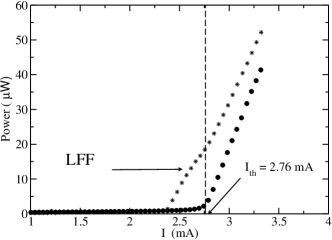
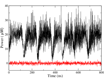
Figure 1: (a) Average power output versus the input current for the solitary laser (dots) and for the laser with feedback (stars). (Color online) (b) Polarization modes: power outputs as a function of time for the VCSEL with feedback at $I=2.64$ mA. Upper trace (black): main polarization; lower trace (red): secondary polarization.

The experimental measurements are performed using a VCSEL semiconductor laser with moderate polarized optical feedback. In particular, our analysis is limited to a regime of pumping below the solitary threshold $I_{th}\sim 2.76$ mA, where the VCSEL emits light on a single linearly polarized transverse mode. Longitudinal modes are not allowed by the cavity, and other transverse modes are not present up to currents $\sim 6.5$ mA. The solitary laser emission remains well polarized up to roughly the same current (see Fig. 1 (b)).

The technical details of the source are the following. The laser is an air-post VCSEL made by CSEM gulden , operating around 770 nm. The mesa diameter is 9.4 $\mu$m, a ring contact defines the ouput window with a diameter of 5 $\mu$m, and the active medium is composed of three 8 nm quantum wells. The temperature of the laser case is stabilized within 1 mK, the pump current is controlled by a home made battery operated power supply whose current noise is below 40 pA/Hz^-1/2 in the frequency range from 1kHz to 3 MHz.

The feedback is applied on the polarization direction of the solitary laser emission. The external cavity includes collimation optics, two polarizers, a variable attenuator, and the feedback mirrors that is mounted on a piezoelectric transducer at about 50 cm from the laser. The output radiation, after optical isolators, is detected by an avalanche photodiode with a bandwidth of about 2 GHz, whose signal, sometimes after low-pass filtering, is recorded by a 4 GHz bandwidth digital scope. More details on the experiment can be found in Refs romanelli ; Soriano2004 .

Optical feedback results in a reduced threshold $I_{th}^{red}\sim 2.42$ mA, as shown in Fig. 1 (a). We have examined the dynamic behavior of the output intensity for various pump currents, both above and below $I_{th}$, with a particular attention to possible effects of the feedback phase $\Delta\phi$ which is varied by acting on the external mirror piezoelectric transducer.

As shown in Fig. 2, we can identify several regimes: (I) at $I<I_{th}$ one observes a single mode LFF dynamics (i.e. the main polarization exhibits LFFs, while the secondary polarization remains off, see Fig. 1 (b)); (II) $I_{th}<I<3.5$ mA: in this regime the LFF dynamics of the main polarization is accompanied by a synchronized spiking behavior in the secondary polarization (coupled modes LFF). This regime was analyzed in Ref. romanelli and, in more details, in Ref. Soriano2004 , where it is proposed that the dynamics of the secondary polarization is driven by the main polarization, whose behavior is not influenced by the orthogonal polarization mode. For larger pump current one begins to observe Coherence Collapse (regime (III) in Fig. 2) and moreover the feedback phase begins to play a fundamental role. In particular, for increasing $I$ in larger and larger portion of the phase interval the laser is stationary (regime (IV) in Fig. 2). This phenomenon is not yet understood and it will be subject of a future analysis loiko .

Anyway, in the present paper we will limit our analysis to regime (I) (i.e. for $I<I_{th}$), where the VCSEL has a single-mode LFF dynamics and the phase delay of the feedback does not play any role. We remark that this statement is suggested by the experiment, where the phase stability would be enough to discriminate such effects, as shown in the analysis of regimes (III-IV).

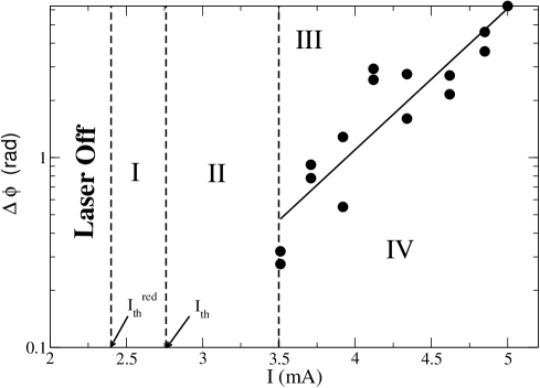
Figure 2: Phase diagram of the VCSEL with feedback: phase of the feedback $\Delta\phi$ as a function of the pump current $I$. The roman numbers denote regions of different dynamical regimes: (I) single-mode LFF, (II) two-mode LFF, (III) coherence collapse and (IV) stable emission. The vertical dashed line indicates (from low to high current) successive current thresholds: the reduced one $I^{red}_{th}$, the solitary laser one $I_{th}$ and the current value separating LFF from coherence collapse. The dots represent the maximal $\Delta\phi$ for which the laser emission remains stable, while the solid line is a guide for eyes to distinguish regions (III) from (IV).

III Numerical model and methods

The dynamics of the VCSEL for $I<I_{th}$ is a purely single mode dynamics and therefore we expect that it could be reproduced by employing the Lang-Kobayashi (LK) LK rate equations for the complex field $E(t)$ and the carrier density $n(t)$. In order to achieve an accurate and reliable comparison of the numerical results with the experimental ones we will employ for our simulations the laser working parameters reported in Table 1. These parameters have been determined via a series of suitable experiments for exactly the same VCSEL employed to obtain the measurements examine in this paper bar05 . The only lacking parameter that was not possible to obtain in the previous characterization is the feedback strength, which is however determined from the threshold reduction.

In this article we use the rate equations derived in Ref. bar05 for the single-mode solitary laser, modified to include the feedback. Defining the deviation $\Delta n$ of the carrier density from transparency normalized to have unitary value at threshold, i.e.

$$\Delta n=\frac{n-1}{n_{th}-1}\qquad,$$ (1)

the following form is obtained bar05 :

$$\tau_{n}\dot{\Delta n} = -\Delta n+1+\eta(\mu-1)-\Delta n|E|^{2}$$

$$\dot{E} = \frac{1+i\alpha}{2\tau_{p}}[\Delta n-1]E+\frac{k}{\tau_{p}}{\rm e}^{-i\omega\tau}E(t-\tau)+\sqrt{R_{0}}\tilde{\xi}(t)$$ (2)

where $\tilde{\xi}(t)=\xi_{R}(t)+i\xi_{I}(t)$ is a complex Gaussian noise term with zero mean and correlation given by $<\xi_{R}(t)\xi_{R}(0)>=<\xi_{I}(t)\xi_{I}(0)>=\delta(t)$ and $<\xi_{R}(t)\xi_{I}(0)>=0$. The noise variance $R_{0}=(n/n_{th})^{2}R_{sp}$ represents a multiplicative noise term proportional to the square of the reduced carrier density $n/n_{th}$ ($n_{th}$ being the threshold carrier density) and to the variance of the spontaneous emission noise $R_{sp}$. The parameter $\mu=I/I_{th}$ is the pump current rescaled to unity at threshold, $\tau_{n}$ and $\tau_{p}$ are carrier and photon lifetimes, respectively, $\tau$ is the delay (or external roundtrip time), $\alpha$ is the linewidth enhancement factor and $\eta$ the reduced gain (for the exact definitions of these quantities in terms of the laser parameters and for the approximations employed to derive (2) see Ref. bar05 ).

By reexpressing the time scale in terms of the photon life-time ($\tau_{p}$) the equations assume the usual form for the LK model and read as

$$T{\dot{\Delta}n} = -\Delta n+p-\Delta n|E|^{2}$$

$$\dot{E} = \frac{1+i\alpha}{2}[\Delta n-1]E+k{\rm e}^{-i\omega\tau}E(t-\tau)+\sqrt{R}\tilde{\xi}(t)$$ (3)

where $T=\tau_{n}/\tau_{p}$, $p=1+\eta(\mu-1)$ and $R=(n/n_{th})^{2}R_{sp}\times\tau_{p}$.

The complex field can be expressed as $E(t)=A(t)+iB(t)=\rho(t)\exp{i\psi(t)}$ and the equations can be rewritten as:

$$\dot{A}(t) = \left(\frac{\Delta n(t)-1}{2}\right)\left(A(t)+\alpha B(t)\right)+k[A(t-\tau)\cos{\phi}+B(t-\tau)\sin{\phi}]+\sqrt{R/2}\xi_{R}(t)$$

$$\dot{B}(t) = \left(\frac{\Delta n(t)-1}{2}\right)\left(B(t)-\alpha A(t)\right)+k[B(t-\tau)\cos{\phi}-A(t-\tau)\sin{\phi}]+\sqrt{R/2}\xi_{I}(t)$$

$$T{\Delta\dot{n}}(t) = p-\Delta n(t)\left[1+A^{2}(t)+B^{2}(t)\right]$$ (4)

where $\phi=\omega\tau$.

Moreover, by assuming that $n\sim n_{th}$ the noise terms become additive with an adimensional variance $R=2.76\times 10^{-3}$, the other quantities entering in (4), expressed in $\tau_{p}$ units, are $\tau=302.5$, $\omega\times\tau=8.743\times 10^{6}$ and $T=30.8333$, the numerical values have been obtained by employing the parameters values in Table  1.

In order to reproduce the power-current response curve for two different experimental data sets we have chosen feedback strengths $k=0.25$ and 0.35, while typically we considered pump currents and linewidth enhancement factors in the range $0.9\leq\mu\leq 1.20$, and $3\leq\alpha\leq 5$, respectively.

The deterministic equations (4) with $R\equiv 0$ have been integrated by employing the method introduced by Farmer in 1982 farmer equipped with a standard 4th order Runge-Kutta scheme, while for integrating the equations with the stochastic terms we have employed an Heun integration scheme toral . The simulations have been performed by integrating the field variables with time steps of duration $\Delta t=\tau/(N-1)$, with $N=1,000-10,000$.

The dynamical properties of the system can be estimated in terms of the associated Lyapunov spectrum, that fully characterizes the linear instabilities of infinitesimal perturbations of the reference system. By following the approach reported in farmer , we have estimated the Lyapunov spectrum $\{\lambda_{k}\}\quad(k=1,\dots,2N+1)$ by integrating the linearized dynamics associated to eqs (4) in the tangent space and by performing periodic Gram-Schmidt ortho-normalizations according to the method reported in benettin . The Lyapunov eigenvalues $\lambda_{k}$ are real numbers ordered from the the largest to the smallest, a positive maximal Lyapunov $\lambda_{1}$ is a indication that the dynamics of the system is chaotic. Moreover, from the knowledge of the Lyapunov spectrum it is possible to obtain an estimation of the number of degrees of freedom actively involved in the chaotic dynamics in terms of the Kaplan-Yorke dimension ky :

$$D_{KY}=j+\frac{\sum_{k=1}^{j}\lambda_{k}}{|\lambda_{j+1}|}$$ (5)

where $j$ is the maximal index for which $\sum_{k=1}^{j}\lambda_{k}\geq 0$.

Table 1: Experimental values of the parameters entering in the model (2) (from bar05 ).

Description	Symbol	Value
Linewidth enhancement factor	$\alpha$	$3.2\pm 0.1$
Photon lifetime in the cavity	$\tau_{p}$	$12\pm 1\enskip ps$
Carrier lifetime	$\tau_{n}$	$0.37\pm 0.02\enskip ns$
External roundtrip time	$\tau$	$3.63\enskip ns$
Variance of the spontaneous emission noise	$R_{sp}$	$(2.3\pm 0.6)\times 10^{-4}\enskip ps^{-1}$
Reduced gain	$\eta$	$5.8\pm 0.6$

IV Stationary Solutions

A first characterization of the phase space of the LK system can be achieved by individuating the corresponding stationary solutions and by analyzing their stability properties. The stationary solutions of the above set of equations can be found by setting $\dot{\rho}=\Delta\dot{n}=0$ and ${\dot{\psi}}=\Omega$, i.e. by looking for solutions of the form

$$E_{S}(t)=\rho_{S}{\rm e}^{i\Omega t}\qquad{\rm and}\qquad\Delta n(t)=\Delta n_{S}\quad.$$ (6)

The stationary solutions can be parametrized in terms of the variable $\theta=\phi+\Omega\tau$, and by setting $J=(p-1)/2$ they can be expressed as follows yanchuk

$$X_{S}=\frac{(\Delta n_{S}-1)}{2}=-k\cos(\theta)$$ (7)

$$\rho_{S}^{2}=2\frac{J-X_{S}}{2X_{S}+1}\geq 0$$ (8)

and

$$\Omega=\frac{\theta-\phi}{\tau}=-k\sqrt{1+\alpha^{2}}\sin(\theta+\theta_{0})$$ (9)

where $\theta_{0}={\rm atan}({\alpha})$ and $-\pi<\theta\leq\pi$.

The stationary solutions are usually termed external cavity modes (ECMs) and correspond to stationary lasing states, in the limit of long delay they are densely covering the following ellipse:

$$k^{2}=X_{S}^{2}+(\Omega-\alpha X_{S})^{2}\quad.$$ (10)

The stability properties of these solutions can be obtained by estimating the associated Floquet spectrum $\{\Lambda_{n}\}$, these eigenvalues are typically complex and their number is infinite, due to the delay term present in the LK equations. However, the stability properties of the ECMs are determined by the eigenvalues with the largest real part, in particular by the maximal one $\Lambda^{M}=({\rm Re}\enskip\Lambda^{M},{\rm Im}\enskip\Lambda^{M})$. These can be easily determined by solving the characteristic equation obtained by linearizing around a certain ECM:

$$Z^{2}_{n}[\Lambda_{n}+\varepsilon(1+\rho_{S}^{2})]+2Z_{n}[\Lambda_{n}\cos(\theta)(\Lambda_{n}+\varepsilon(1+\rho_{S}^{2})+\varepsilon\rho_{S}^{2}(1-2k\cos(\theta))(\cos(\theta)-\alpha\sin(\theta))/2]$$ (11)

$$+ \Lambda_{n}^{2}[\Lambda_{n}+\varepsilon(1+\rho_{S}^{2})]+\Lambda_{n}\varepsilon\rho_{S}^{2}(1-2k\cos(\theta))\equiv a_{n}Z^{2}_{n}+2b_{n}Z_{n}+c_{n}=0\quad.$$

where $Z_{n}=k(1-{\rm e}^{-\Lambda_{n}\tau})$ and $\varepsilon=1/T$. The pseudo-continous spectrum ya2 can be obtained by solving eq. (11) in terms of $Z_{n}$ and by considering $\Lambda_{n}$ as a parameter. In this case the solutions of the corresponding second order equation are

$$\Lambda_{n}^{\pm}=-\frac{1}{\tau}\log\left[1+\frac{b_{n}\mp\sqrt{b_{n}^{2}-a_{n}c_{n}}}{ka_{n}}\right]+i2\pi n$$ (12)

and by self-consistently solve the above equation one can find all the eigenvalues, that are arrangend in two branches. However, the spectrum contains also isolated eigenvalues, that can be obtained by solving directly Eq. (11) in terms of $\Lambda_{n}$ and by considering $Z_{n}$ as a parameter. In this case the equation is a cubic and by solving self-consistely its expression one finds (up to) three distinct eigenvalues. While the pseudo-continuos spectrum emerges due to the presence of the delay in the system, the isolated eigenvalues originate from those characterizing the three dimensional single laser rate equations in absence of the delay, i.e., the Eq. (3) with $\tau=0$ ya2 .

Typically, depending on their linear stability properties ECM are divided into modes and antimodes levine . Antimodes are characterized by a positive real eigenvalue and are therefore unstable. For the modes instead the maximal real eigenvalue is zero and they are unstable whenever the associated spectrum crosses the imaginary axis. Various types of instabilities can be observed for these delayed systems and they can be classified for analogy with the spatially extended systems as for example modulational-type or Turing-type instabilities yanchuk ; ya2 . Examples of the unstable branch for the spectra $\{\Lambda_{k}\}$ associated to Turing-type and modulationali-type instabilities are reported in Fig. 3, for a classification of the possible instabilities of equilibria for delay-differential equations see ya2 .

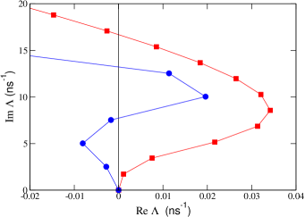
Figure 3: (Color online) Unstable branch $\Lambda$ associated to specific modes of the LK. The mode $\theta=-0.32$ for $\alpha=3.20$ reveals a sort of modulational instability (red squares), while the mode $\theta=-0.08$ for $\alpha=3.22$ shows a Turing-like instability (blue circles). The results refer to $\mu=0.93$. Due to the symmetry of the spectra only the part corresponding to $Im\Lambda>0$ is displayed.

In particular, the modes correspond to $\theta$-values located within the interval $[\theta_{2}:\theta_{1}]$, where $\theta_{1}\sim{\rm atan}(1/\alpha)$ and $\theta_{2}\sim-\pi+{\rm atan}(1/\alpha)$. Moreover, stationary solutions are acceptable only if they correspond to positive intensities $\rho^{2}_{S}\geq 0$, i.e. if they are situated within the interval $[-\theta_{R}:\theta_{R}]$ with $\theta_{R}={\rm acos}{(-J/k)}$. In the range of parameters examined in the present paper the number of stable modes (SMs) is always between two and four and they are located in a narrow interval of $\theta$ located around zero (i.e. around the so called Maximum Gain Mode (MGM)).

As we will report in the following section, by integrating the deterministic version of the model (4) for moderate $\alpha$- and $\mu$-values, we always observe a relaxation towards one of the SMs. In particular for $3<\alpha<5$ the dynamics seem to relax always towards one of the SMs located in proximity of the MGM (corresponding to $\theta\equiv 0$) (see Fig. 4). It should be noticed that the MGM is a solution of the system only for appropriate choices of $\phi$. Two examples of typical ECMs are reported in Fig. 4 for the present system for $\alpha=3.2$ and 5 and $\mu=0.93$, in both cases two stable attracting modes have been identified. Recently, a similar coexistence of two stable solutions located in proximity of the MGM has been reported experimentally for an edge-emitter laser with a low level of optical feedback mendez

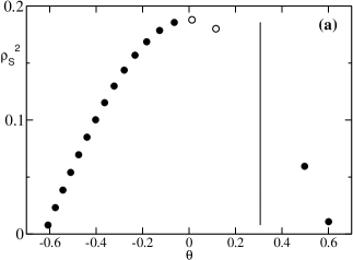
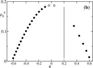
Figure 4: Intensities versus $\theta$ for ECMs of eq. (4) with $\mu=0.93$ and for $\alpha=3.2$ (a) and $5.0$ (b). The solid line indicates $\theta_{1}$. The ECMs with $\theta<\theta_{1}$ are modes, while the others are antimodes. The empty circles indicates the SMs towards which we numerically observed relaxation of the system by considering up to 100 different random initial conditions.

As reported in yanchuk the stability properties of the MGM do not depend on $\alpha$, therefore it is reasonable to expect that some SM will be always present in a narrow window around $\theta$ for any chosen linewidth enhancement factor levine and that they will coexist with the chaotic dynamics, as observed experimentally in heil .

V Deterministic Dynamics

An open problem concerning the deterministic LK equations is if and for which range of parameters these equations faithfully reproduce the experimentally observed dynamics. Particular interest is usually focused on the $\alpha$-value to be employed to obtain a realistic behaviour of the model.

V.1 LFFs as a transient phenomenon

To answer this question we consider the deterministic verson of the model (4) (i.e. by assuming $R\equiv 0$) equipped with the parameter values deduced by the experimental data bar05 apart for $\mu$ and $\alpha$ that will be varied. In particular, we would like to understand if the system shows a LFF behaviour and if such dynamics is statistically stationary or not. In order to verify it, we initialize randomly the amplitude $\rho(t=0)$, the phase $\phi(t=0)$ and the excess carrier density $\Delta n(t=0)$, then we follow the dynamics and we examine the evolution of the field intensity $\rho^{2}(t)$. If the dynamics end up on a stationary solution we register the time $T_{s}$ necessary to reach it and we average this time over many ($M$) different initial conditions. In order to measure $T_{s}$, we estimate the time needed to the standard deviation of the intensity (evaluated over sub-windows of time duration $t_{w}$) to decrease below a chosen threshold $\Gamma$. The average times $<T_{s}>$ are reported in Fig. 5

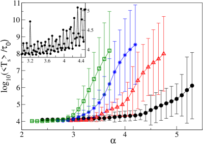
Figure 5: (Color online) Logarithm of the transient times $<T_{s}>$ as a function of $\alpha$ for various $\mu$-values: namely, $\mu=0.93$ (black filled circles), $0.95$ (red empty triangles), $0.97$ (blue asteriskes) and $0.99$ (green empty squares). The data refers to $k=0.25$, $\Gamma=10^{-5}$, $t_{w}=1000\tau=3.630\mu s$ and $M\sim 10-100$, and they have been obtained by employing an integration time step $\Delta t=3.63ps$. The time scale of the figure is $\tau_{0}=1\enskip$ ns. The bars reported for each measured value indicate the range of variability of $<T_{s}>$ (within a $\alpha$-interval of amplitude 0.1) due to its finer structure shown in the inset. In the inset are displayed the transient times for $\mu=0.93$ reported at a higher resolution in $\alpha$, namely for a resolution of $0.02$.

The main result shown in Fig. 5 is that the system after a transitory phase (shorter or longer) settles down to a SM and that the duration of the transient increases for increasing $\alpha$ or $\mu$-values. Preliminary indications in this direction have been previously reported in dfb . These results clearly indicate that the LFF dynamics is just a transient phenomenon for the deterministic LK equation for commonly employed $\alpha$-values (i.e., for $\alpha\sim 3.0-3.5$). For each fixed $\mu$ it seems that $<T_{s}>$ diverge above some ”critical” $\alpha$-value, however we cannot exclude that the system will also in this case finally converge to a SM. At least we can consider the reported critical values as lower bounds above which LFF could occur as a stationary phenomenon and not as a transitory state. With the chosen numerical accuracy and due to the available computational resources, for any pratical purpose a transient longer than $0.1-1$ s can be considered as an infinite time.

An interesting feature is that the variability of $<T_{s}>$ with $\alpha$ is quite wild and it reflects the stability of the modes in proximity of the MGM, as shown in Fig. 6. However the average values $<T_{s}>$ (averaged also over $\alpha$-intervals of width $0.1$) still indicates a clear trend of the transient times to increase with $\alpha$.

We expect that the time scale associated to the convergence to a stable mode is ruled by the eigenvalue with the maximal real part (apart the eigenvalue zero, that is always present due to the phase invariance of the LK equations). In particular we expect that the intensity of the signal will converge towards the stable mode as

$$\rho^{2}(t)\sim\rho^{2}(0){\rm e}^{\rm 2Re\enskip\Lambda^{M}\enskip t}cos(\rm 2Im\enskip\Lambda^{M}\enskip t)+\rho_{S}^{2}$$

where $\Lambda^{M}$ is the eigenvalue with maximal (non zero) real part associated to the considered stable solution. For small $\mu$ we have observed that the dynamics can collapse to different stable solutions (typically, from 1 to 3). By estimating the probability $P_{m}=N_{m}/M$ to end up in one of these states (being $N_{m}$ the number of initial conditions converging to the $m$-mode) and by indicating the corresponding eigenvalue with maximal real part as $\Lambda^{M}(m)$, a reasonable estimate of $<T_{s}>$ is given by

$$T_{est}=\frac{\ln{\Gamma}}{2}\sum_{m}\frac{P_{m}}{|\rm Re\Lambda^{M}(m)|}\quad,$$ (13)

where $\Gamma$ is the employed threshold. As it can be seen in Fig. 6, the estimation is quite good and the periodicity of the two quantities is identical in the examined range of $\alpha$-values and for $\mu=0.93$. The expression (13) always gives a good estimate of $<T_{s}>$ for $\alpha<4$ and for $\mu<1$, but the agreement worsens for increasing $\alpha$-values.

However, even a more rough estimate is capable to give a reasonable approximation of $<T_{s}>$ and in particular to capture its periodicity. This estimate is simply given by

$$T_{1}=\frac{\ln{\Gamma}}{2}\frac{1}{|\rm Re\bar{\Lambda}^{M}|}\quad,$$ (14)

where $\bar{\Lambda}^{M}$ is the eigenvalue with maximal non zero real part associated to the stable mode with higher $\theta$ (i.e. the first stable mode located in proximity of the anti-mode boundary).

From the present analysis it emerges that the stable modes play a relevant role for the (transient) dynamics of the deterministic LK equations at least for $\alpha<4$. Moreover the observed strongly fluctuating behaviour of $<T_{s}>$ as a function of $\alpha$ indicates that the choice of this parameter is quite critical, since a small variation can lead to an increase of an order of magnitude of the transient time

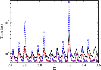
Figure 6: (Color online) Transient times $<T_{s}>$ (black filled circles), $T_{est}$ (red empty triangles) and $T_{1}$ (blue empty square) in nanoseconds as a function of $\alpha$. The results have been obtained by examining the decay of $\rho^{2}(t)$ with $\Gamma=10^{-5}$ and $t_{w}=1000\tau=3.630\mu s$ and $M\sim 100-500$. The employed integration time step is $\Delta t=0.363$ ps and the data refer to $k=0.25$ and $\mu=0.93$.

V.2 Lyapunov Analysis

We have characterized the transient dynamics preceeding the collapse in the stationary state in terms of the maximal Lyapunov $\lambda_{1}$ and of the associated Kaplan-Yorke (or Lyapunov) dimension $D_{KY}$. In particular, these quantities reported in Fig. 7 have been estimated by integrating the linearized dynamics for a sufficiently long time period $T_{int}$ and by averaging over $M$ different initial realizations.

It is clear from the figures that the average maximal Lyapunov exponent $<\lambda_{1}>$ is definetely not zero for all the considered situations and that it increases (almost steadily) with the parameter $\alpha$ as well as with the pump parameter. Moreover, also this indicator reflects the stability properties of the SMs located in proximity of the MGM, by exhibiting large oscillations as a function of $\alpha$, as shown in the inset of 7(a).

The values of $<D_{KY}>$ reported in 7(b) clearly indicate that the system cannot be described as low dimensional, even during the transient and even below the solitary laser threshold. As a matter of fact the number of active degrees of freedom ranges between $10$ and $50$. It should be noticed that $<D_{KY}>$ is determined by the instability properties not only of anti-modes and but also of modes that have bifurcated (via Hopf instabilities) becoming unstable for increasing $\alpha$.

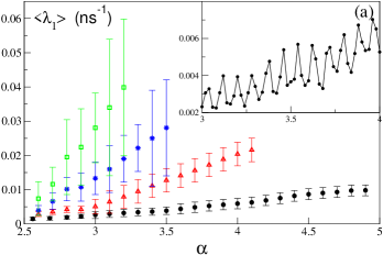
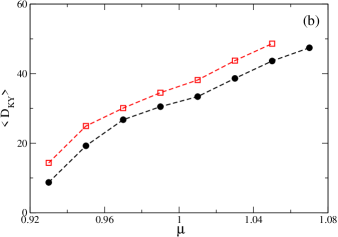
Figure 7: (Color online) (a) Average maximal Lyapunov exponents $<\lambda_{1}>$ as a function of $\alpha$ and for various $\mu$-values below threshold: namely, $\mu=0.93$ (black filled circles), $0.95$ (red empty triangles), $0.97$ (blue asterisks) and $0.99$ (green empty squares). The bars reported for each measured value indicates the range of variability of $<\lambda_{1}>$ due to its finer structure as measured within a $\alpha$-interval of width 0.1. In the inset the data for $<\lambda_{1}>$ are reported for a higher resolution in $\alpha$ (namely 0.02) for $\mu=0.93$. (b) Average Kaplan-Yorke dimensions $<D_{KY}>$ as a function of $\mu$ for $\alpha=4$ (black filled circles) and 5 (red empty squares). All the data refer to $k=0.25$, for the $<\lambda_{1}>$ estimation $\Delta t=0.363$ ps, $M=500$, and $T_{int}=3.63$ ms while for the $<D_{KY}>$ evaluation $\Delta t=3.63$ ps, $M=20$ and $T_{int}=0.14$ ms.

VI Noisy Dynamics

We have examined the dynamics (2) for increasing level of noise, namely for $10^{-6}<R<10^{-2}$. Also in this case, for $\alpha=3.3$ and for noise levels smaller than $10^{-3}$ the LFF dynamics only occurs during a transient. However for increasing $R$ values we observed a transition to sustained LFF and the transition region was characterized by an intermittent behaviour. These behaviours are exemplified in Fig. 8 for $\alpha=3.3$ and $\mu=0.97$. As shown in Fig. 8(a) the orbit spends long times in proximity of one of the SM and then, due to noise fluctuations, escapes from the attraction basin associated to the stable solution and exhibit LFFs before being newly reattracted by the SM. This intermittent dynamics can be interpreted as an activated escape process induced by noise fluctuations, and therefore the average residence time $<T_{res}>$ in the attraction basin of the SM can be expressed in the following way

$$<T_{res}>\propto\exp{[W/R]}$$ (15)

where $W$ represent a barrier that the orbit should overcome in order to escape from the SM valley. As shown in Fig. 9 the process can be indeed interpreted in terms of the Kramers expression (15) for $2\times 10^{-4}<R<7\times 10^{-4}$. It means that for $R<W$ one should expect an intermittent behaviour, while for $R>W$ the dynamics of the orbit will be essentially diffusive, since the noise fluctuations are sufficient to drive the orbit always out of the SM valley. These indications suggest that in order to observe a “non transient” or “non intermittent” LFF dynamics the amount of noise present in the system should be larger than $W$. Also in dfb it has been clearly stated that the LK-equations with parameters tuned to reproduce the dynamics of a DFB laser with $\alpha=3.4$ can give rise to stationary LFF only in presence of noise.

It is important to remark that for $\alpha=3.3$ the experimentally measured variance of the noise $R=2.76\times 10^{-3}$ is above the barrier $W=1.87\times 10^{-3}$ found from the fit of the numerical $<T_{res}>$ with expression (15), performed in the small noise range (see Fig. 9). Moreover in the experiments we never observed relaxation of the dynamics towards a SM.

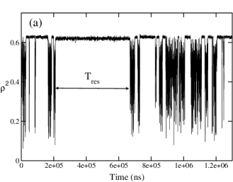
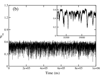
Figure 8: Intensity of the field $\rho^{2}$ as a function of the time for the noisy LK equations. The data have been filtered with a low-pass filter at $80$ MHz and refer to $\mu=0.97$, $\alpha=3.3$. The results reported in (a) correspond to a noise variance $R=3\times 10^{-4}$, while those in (b) are relative to $R=3\times 10^{-3}$. In (a) a typical time of residence $T_{res}$ around one of the SMs is indicated. The inset in (b) is an enlargement of the actual dynamics.

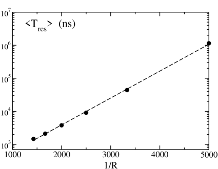
Figure 9: Average residence times in the SM as a function of the inverse of the variance of the additive noise to the LK equations. The dashed line is a exponential fit $\propto\exp{[W/R]}$ to the numerical data, the fitted exponential slope is $W=0.00187$. The data refer to $\mu=0.97$ and $\alpha=3.3$.

VI.1 Lyapunov Analysis

Also in the noisy case we have examined the degree of chaoticity in the system by estimating the maximal Lyapunov exponent along noisy orbits of the system. The role of noise is fundamental in destabilizing the dynamics of the system and in rendering the asymptotic dynamics chaotic.

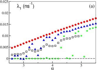
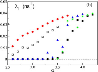
Figure 10: (color online) Maximal Lyapunov exponents $\lambda_{1}$ as a function of $\alpha$ for $\mu=0.93$ (a) and $\mu=0.97$ (b) and for various noise amplitude $R$: namely, the data for $R=3\times 10^{-5}$ are indicated by green asterisxs, those for $R=3\times 10^{-4}$ by blue filled triangles, and the ones corresponding to $R=3\times 10^{-3}$ by red filled circles. The values estimated during the transient dynamics in absence of noise are indicated by black empty squares, while the asymptotic values for $R=0$ by black filled squares. All the data refer to $k=0.25$, for the estimation of $\lambda_{1}$ in the noisy case one orbit has been followed for a time $t=3.63$ ms with time step $\Delta t=0.363$ ps, while in the deterministic case the asymptotic results have also been averaged over $M=10$ different initial conditions. For details on the estimation of the transient Lyapunov exponents see the previous section V.2.

In particular, as shown in Fig. 10(a) we observe that at $\mu=0.93$ and $k=0.25$ the deterministic dynamics ($R=0$) is asymptotically stable in the range $\alpha\leq 4.4$, while the noisy dynamics becomes more and more chaotic for increasing $R$. For the value $R=3.3\times 10^{-3}$, close to the experimental one, the dynamics is completely destabilized in the whole examined range $2.5\leq\alpha\leq 4.5$, while for smaller $R$-values the range of destabilization is reduced. These results confirm the role of the noise in rendering the LFF an asymptotic phenomenon. Moreover the maximal Lyapunov increeases steadily with $\alpha$ at $R=3.3\times 10^{-3}$. Similar findings apply in the case $\mu=0.97$ (see Fig. 10(b)).

The wild oscillations in the $<\lambda_{1}>$ values observable at level of noise $R<10^{-4}$ reflect the stability properties of the SMs attracting the asymptotic dynamics.

VII Comparison between experimental and numerical data

This Section will be devoted to a detailed comparison of numerical versus experimental results with the aim to clarify if the deterministic or noisy LK eqs are indeed able to reproduce the experimental findings.

VII.1 Distributions of the field intensities

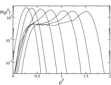
Figure 11: Field intensities distributions $P(\rho^{2})$ for the experimental signal filtered at 200 MHz. The experimental intensities have been arbitrarly rescaled to match the corresponding average intensities obtained from the simulation of the noisy LK eqs at $\alpha=3.3$ and $k=0.35$ with noise variance $R=3.3\times 10^{-3}$. The data refer from left to rigth to $I=2.48$ mA, 2.50, 2.54, 2.58, 2.64, 2.70, and 2.75. Since $I_{th}=2.76$ these data correspond to $0.9<\mu<1.0$. The first distribution has a large contribution from the Gaussian electronic noise, which also explains the negative $\rho^{2}$ values.

As a first indicator we have considered the distribution of the field intensities $P(\rho^{2})$, in particular in order to match the experimental findings we consider the signal filtered at 200 MHz.

The experimental results for the probability distribution functions (PDFs) of the field intensities $\rho^{2}$ are reported in Fig. 11 for various currents below the solitary threshold value. It should be noticed that the amplitudes $\rho^{2}$ have been rescaled in order to match the corresponding numerical values for the noisy LK eqs with $\alpha=3.3$ and noise variance $R=3.3\times 10^{-3}$, but that no arbitrarly shift have been applied to the data.

A peculiar characteristic of these data is that for increasing pump current the PDFs become more and more asymmetric, revealing a peak at large intensities that shifts towards higher and higher $\rho^{2}$ values and a sort of plateau at smaller intensities.

The corresponding PDFs are reported in Figs. 12 and 13 for data obtained from the integration of the noisy and deterministic LK eqs, respectively. A better agreement between numerical and experimental findings is found for the noisy dynamics with $\alpha\sim 3.3-4.0$ and $k=0.35$, with a noise variance similar to the experimental one (namely, $R=3\times 10^{-3}$). For the deterministic case (reported in Fig. 13 for $\alpha=5.0$ and $k=0.35$) a non zero tail at $\rho\sim 0$ is observed even for $\mu\sim 1.0$, contrary to what observed for the experimental data.

These results indicate that it is necessary to include the noise in the LK eqs to obtain a reasonable agreement with the experiment, at least at the level of the intensities PDFs. However, the numerical data seem unable to reproduce the narrow peak present in the experimental ones at large intensities and for $\mu\to 1$. In the next sub-section a further comparison will be performed to validate these preliminary indications.

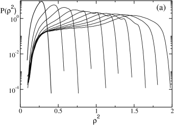
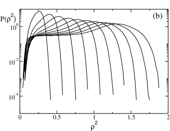
Figure 12: Field intensities distributions $P(\rho^{2})$ for the numerical data obtained by the integration of a noisy LK eqs. filtered at 200 MHz. The data refer from left to rigth to $\mu=0.90$, 0.91, 0.92, 0.93, 0.94, 0.95, 0.96, 0.97, 0.98, and 0.99 for (a) $\alpha=3.3$ and (b) $\alpha=4.0$. Both the sets of data correspond to $k=0.35$ and noise variance $R=3\times 10^{-3}$.

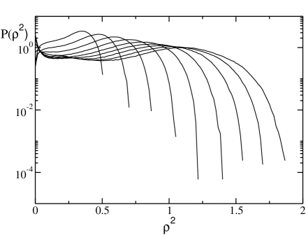
Figure 13: Field intensities distributions $P(\rho^{2})$ for the numerical data obtained by the integration of a deterministic LK eqs. filtered at 200 MHz. The data refer from left to rigth to $\mu=0.91$, 0.92, 0.93, 0.94, 0.95, 0.96, 0.97, 0.98, and 0.99 for $\alpha=5.0$ and $k=0.35$.

VII.2 Average values of the LFF times

We will first compare the experimental and numerical measurements of the average times between two consecutive drops of the field intensities $<T_{LFF}>$. They have been evaluated in two (consistent) ways: both from a direct measurement of periods between threshold crossing, and from the Fourier power spectrum of the temporal signal $\rho^{2}(t)$.

The direct measurements of the $T_{LFF}$ from the time trace of $\rho^{2}(t)$ have been performed by defining two thresholds $\Gamma_{1}<\Gamma_{2}$ and by identifing two consecutive time crossing of $\Gamma_{1}$, provided that in the intermediate time the signal has overcome the threshold $\Gamma_{2}$ at least once. The thresholds have been defined as $\Gamma_{1}=<\rho^{2}>-2*STD$ and $\Gamma_{2}=<\rho^{2}>+STD/2$, where $<\cdot>$ and STD indicate the average and the standard deviation of the signal itself.

The measurement of $<T_{LFF}>$ in terms of the power spectrum has been obtained by considering the power spectrum $S(\omega)$ of $\rho^{2}(t)$ and by evaluating the position $\omega_{M}$ of the peak with the highest frequency, then $<T_{LFF}>=2\pi/\omega_{M}$. As already mentioned the two estimations are generally in very good agreement.

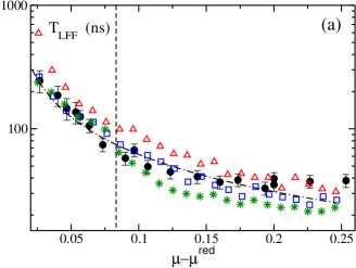
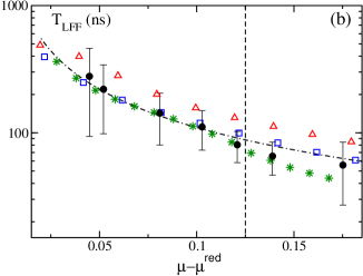
Figure 14: (Color online) Average LFF times $<T_{LFF}>$ as a function of the pump parameter $\mu-\mu^{red}$: black filled circles refer to experimental data, while the other symbols to the results obtained from the integration of the LK eqs. In the two figures are reported two different sets of experimental measures and the associated numerical data refer to $k=0.25$ (a) and $k=0.35$ (b). In particular, red empty triangles correspond to the evolution of the noisy LK at $\alpha=3.3$ (with (a) $\mu^{red}=0.914$ and (b) $\mu^{red}=$0.880) and blue empty squares to $\alpha=4.0$ (with $\mu^{red}=0.913$ and 0.878, resp. for (a) and (b)). In both cases $R=3\times 10^{-3}$. The green stars denote the data of the deterministic LK eqs for $\alpha=5.0$ (in this case $\mu^{red}=0.915$ and 0.882, resp. for (a) and (b)). For the experimental measures $\mu^{red}=0.916$ in (a) and 0.875 in (b). The vertical dashed lines indicates the position of the solitary threshold for the experimental data, while the dash-dotted lines represent the decay $c/(\mu-\mu^{red})$, with $c=6.2$ ns and 11 ns in (a) and (b), respectively. $\mu^{red}$ is defined as the ratio $I^{red}_{th}/I_{th}$.

In Fig. 14 the average times $<T_{LFF}>$ are reported for two different sets of experimental measurements as a function of the pump parameter $\mu$ and compared with numerical data. In Fig. 14 (a) are reported the experimental findings already shown in romanelli , the estimation of $T_{LFF}$ have been performed both by direct inspection of the signal and via the first zero of the autocorrelation function (this second method corresponds to an evaluation from the Fourier power spectrum). The numerical data have been obtained with the 2 methods outlined above for $k=0.25$ for both noisy and deterministic LK eqs. In Fig. 14 (b) a new set of experimental data is reported and compared with simulation results for $k=0.35$, in this case all the data have been obtained by the method of the thresholds. From the figures it is clear that a reasonably good agreement between experimental and numerical data is observed for the deterministic case only for $\alpha=5$ (results for smaller $\alpha$-values, obtained during the transient preceeding the stable phase, are not shown but they exhibits a worst agreement with experimental findings) and for the noisy dynamics for $\alpha=4.0$.

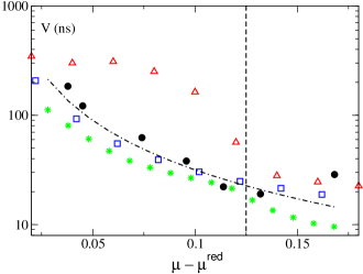
Figure 15: (Color online) Standard deviation of the LFF times $V$ as a function of the pump parameter $\mu-\mu^{red}$: the symbols are the same as those reported in Fig. 14 (b). The dash-dotted line indicates the power-law decay $1/(\mu-\mu^{red})^{3/2}$.

A more detailed analysis can be obtained by considering not only the average values of the LFF times, but also the associated standard deviation $V$. This quantity reported in Fig. 15 exibits a clear decrease with $\mu$ by approaching the solitary treshold, indicating a modification of the observed dynamics that tends to be more “regular”. Also in this case the comparison of experimental and numerical data suggests that the best agreement is again attained with the noisy dynamics at $\alpha=4.0$.

At this stage of the comparison we can sketch some preliminary conclusions: the LK eqs are able to reproduce reasonably well the experimental data for the VCSEL below the solitary threshold both in the deterministic case and in the noisy situation. However in the deterministic case a quite large value of the linewidth enhancement factor (with respect to the experimentally measured one) is required. A more detailed comparison will be possible by considering the PDFs of the $T_{LFF}$.

VII.3 Distributions of the LFF times

In this sub-section we will examine the whole distribution of the $T_{LFF}$ in more details. Considering the experimental data, we observe that all the measured PDFs obtained for different pump currents reveal an exponential-like tail at long times and a rapid drop at short times (as shown in Fig. 16). These results are in agreement with those reported in sukov for a single-transverse-mode semiconductor laser in proximity of $I_{th}$.

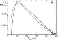
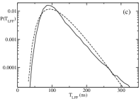
Figure 16: Probability density distributions of the $T_{LFF}$. Solid lines refer to experimental data, the dashed ones to the Inverse Gaussian Distribution (18) with the average and standard deviation corresponding to the experimental ones. (a) $I=2.56$ mA, (b) $I=2.64$ mA, and (c) $I=2.70$ mA

The typical dynamics corresponding to a LFF can be summarized as follows: a sudden drop of the intensity is followed by a steady increase of $\rho^{2}$, associated to fluctuations of the intensity, until a certain threshold is reached and the intensity is reset to its initial value and restart with the same “sysiphus cycle” sano . This behaviour and the observed shapes of the PDFs suggest that the dynamics of the intensities can be modelized in terms of a Brownian motion plus drift. In other words, by denoting with $x(t)$ the intensity, an effective equation of the following type can be written to reproduce its dynamical behaviour:

$$\dot{x}(t)=\eta+\sigma\xi(t)$$ (16)

with initial condition $x(0)=x_{0}$, where $\xi(t)$ is a Gaussian noise term with zero average and unitary variance, $\eta$ represents the drift, $\sigma$ is the noise strength. Within this framework the average first passage time to reach a fixed threshold $\Gamma$ is simply given by $\tau=(\Gamma-x_{0})/\eta$ , while the corresponding standard deviation is $V=[\sqrt{(\Gamma-x_{0})}\sigma]/\eta^{3/2}$ tuckwell . A resonable assumption would be that $\eta$ is directly proportional to the pump parameter $(\mu-\mu^{red})$, (where $\mu^{red}=I^{red}_{th}/I_{th}$ is the rescaled pump current value at the reduced threshold) and by further assuming that the threshold $\Gamma$ is independent on the pump current this would imply that

$$<T_{LFF}>=\frac{c}{(\mu-\mu^{red})}\qquad,\quad{\rm and}\quad V_{LFF}=\frac{c}{(\mu-\mu^{red})^{3/2}}$$ (17)

these dependences are indeed quite well verified for the experimental data above the solitary threshold as shown in Figs 14 and 15.

For the simple model introduced by eq. (16), the PDF of the first passage times is the so-called Inverse Gaussian Distribution gaussiana :

$$P(T)=\frac{\tau}{\sqrt{2\pi\gamma T^{3}}}{\rm e}^{-(T-\tau)^{2}/(2\gamma T)}$$ (18)

where $\gamma=V^{2}/\tau$. A comparison of this expression with the experimentally measured $P(T_{LFF})$ is reported in Fig. 16. The good agreement suggests that the “sysiphus cycles” can be due to few elementary ingredients: a stochastic motion subjected to a drift plus a reset mechanism once the intensity has overcome a certain threshold.

A way of rewriting the distribution (18) in a more compact form as a function of only one parameter, the so-called coefficient of variation $\delta=V/\tau$ (i.e., the ratio between the standard deviation $V$ and the mean $\tau$), is to rescale the time as $z=(T-\tau)/V$ and the PDFs as $g(z)=V*P(T)$. This procedure leads to the following expression:

$$g(z)=\frac{1}{\sqrt{2\pi(\delta z+1)^{3}}}{\rm e}^{-z^{2}/2(\delta z+1)}\quad.$$ (19)

It is clear that all the PDFs will coincide, once rescaled in this way, if the coefficient of variation $\delta$ has the same value for all the considered pump currents. However this is not the case and indeed we measured values of $\delta$ in the range $[0.28:0.66]$ for $I<I_{th}$, nonetheless if we report in a single graph all these curves the overall matching is very good, as shown in Fig. 17.

Figure 17: Rescaled probability density distributions $g(z)=V*P(T_{LFF})$ as a function of $z=(T_{LFF}-<T_{LFF}>)/V$. The curves refer to $I=2.54$ mA, 2.56 mA, 2.64 mA, 2.70 mA, 2.75 mA, 2.80 mA, and 2.90 mA.

Let us finally compare these distributions $g(z)$ with the corresponding ones obtained from direct simulations of the LK eqs.. As one can see from Fig. 18 the agreement is good for the data obtained from the simulation of the noisy LK eqs at $\alpha=4.0$, while it is worse for the deterministic LK eqs at $\alpha=5.0$.

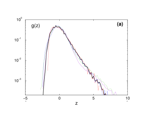
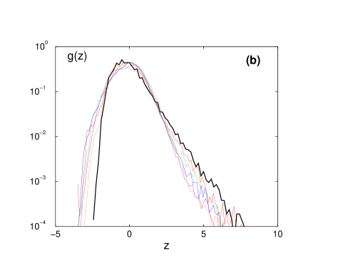
Figure 18: (Color line) Rescaled probability density distributions $g(z)=V*P(T_{LFF})$ as a function of $z=(T_{LFF}-<T_{LFF}>)/V$. The thick solid curve refer to experimental data for $I=2.75$ mA (corresponding to $\mu\simeq 1$), the other ones to numerical findings: (a) data obtained for the noisy LK eqs for $\alpha=4.0$, $k=0.35$ with variance $R=3\times 10^{-3}$ and corresponding to $\mu=0.90$ (red), 0.94 (blue), 0.98 (green), and 1.02 (violet); (b) data for the the deterministic LK eqs. for $\alpha=5.0$, $k=0.35$ corresponding to $\mu=0.92$ (red) , 0.94 (blue), 0.96 (green), 0.98 (violet), and 1.00 (orange).

VIII Conclusions

We presented a detailed experimental and numerical study of a semiconductor laser with optical feedback. The choice of a Vertical Cavity Laser pumped close to its threshold, together with a polarized optical feedback, assures a great control over the possibility of lasing action of other orders longitudinal and/or transverse modes than the fundamental one, and of the activation of the other polarization. In such a way, the description of the system using the Lang-Kobayashi model is well justified and it allows for a meaningful comparison with the experimental data. The analysis has been performed with particular regard to the LFF regime, where the model has been numerically integrated using parameters carefully measured in the laser sample used for the measurements.

The comparison of the the measurements carried out in the VCSEL with polarized optical feedback with the predictions of the deterministic LK model suggest that in the examined range of parameters the dynamics of the model is characterized by a chaotic transient leading to stable ECMs with high gain. The transient duration increases (and possibly diverges) with increasing values of the rescaled pump current $\mu$ and of the linewidth enhancement factor $\alpha$. We have not found evidence of periodic or quasi-periodic asymptotic attractors, as instead reported in david , this can be due to the $\alpha$-range examined in the present paper (namely $2.4\leq\alpha\leq 5.5$), since these solutions become relevant for the dynamics only for $\alpha>5$ (as stated in david ).

However, a stationary LFF dynamics with characteristics similar to those measured experimentally, can be obtained for realistic values of the $\alpha$ parameter (namely, $\alpha\sim 3-4$) only via the introduction of an additive noise term in the LK equations. The role of noise in determining the statistics and the nature of the dropout events has been previously examined in hk ; hohl , but in the present paper we have clarified that the LFF dynamics can be interpreted at a first level of approximation as a biased Brownian motion towards a threshold with a reset mechanism.

- (1) C. Risch and C. Voumard, J. Appl. Phys. 48 (1977) 2083.
- (2) Fundamental issues of nonlinear laser dynamics, AIP Conference Proceedings CP548, eds B. Krauskopf and D. Lenstra (New York, 2000).
- (3) C.H. Henry and R.F. Kazarinov, IEEE J. Quantum. Electron. QE-22 (1986) 294.
- (4) A. Hohl, H.J.C. van der Linden, and R. Roy, Opt. Lett. 20 (1995) 2396.
- (5) T. Sano, Phys. Rev. A50 (1994) 2719.
- (6) R.L. Davidchack, Y-C. Lai, A. Gavrielides, and V. Kovanis, Phys. Rev. E63 (2001) 056206.
- (7) T.W. Carr, D. Pieroux, and P. Mandel, Phys. Rev. A63 (2001) 033817.
- (8) I. Pierce, P. Rees, P.S. Spencer, Phys. Rev. A61 (2000) 053801
- (9) E.A. Viktorov and P. Mandel, Phys. Rev. Lett. 85 (2000) 3157.
- (10) G. Huyet, S. Balle, M. Giudici, C. Green, G. Giacomelli, and J.R. Tredicce, Opt. Commun. 149 (1998) 341.
- (11) G. Vaschenko, M. Giudici, J.J. Rocca, C.S. Menoni, J.R. Tredicce, and S. Balle, Phys. Rev. Lett. 81 (1998) 5536.
- (12) A. A. Duarte and H. G. Solari, Phys. Rev. A 64, 033803 (2001), Phys. Rev. A 60, 2403-2412 (1999), Phys. Rev. A 58, 614-619 (1998)
- (13) M. Giudici, C. Green, G. Giacomelli, U. Nespolo, and J. R. Tredicce, Phys. Rev. E 55, 6414 (1997).
- (14) T. Heil, I. Fischer, W. Elsässer, J. Mulet, and C. R. Mirasso, Opt. Lett. 24 (1999) 1275.
- (15) G. Giacomelli, F. Marin, and M. Romanelli, Phys. Rev. A67 (2003) 053809.
- (16) G. Vaschenko, M. Giudici, J. J. Rocca, C. S. Menoni, J. R. Tredicce, and S. Balle, Phys. Rev. Lett. 81, 5536 (1998)
- (17) D.W. Sukow, T. Heil, I. Fischer, A. Gavrielides, A. Hohl-AbiChedid, and W. Elsässer, Phys. Rev. A60 (1999) 667.
- (18) D.W. Sukow, J.R. Gardner, and D. J. Gauthier, Phys. Rev. A56 (1997) R3370.
- (19) J. Mulet and C.R. Mirasso, Phys. Rev. E59 (1999) 5400.
- (20) W-S Lam, W. Ray, P.N. Guzdar, and R. Roy, Phys. Rev. Lett. 94 (2005) 010602.
- (21) R. Lang and K. Kobayashi, IEEE J. Quantum Electronics 16 (1980) 347
- (22) F. Rogister, M. Sciamanna, O. Deparis, P. Mégret, and M. Blondel, Phys. Rev. A65 (2001) 015602.
- (23) M. Giudici, S. Balle, T. Ackemann, S. Barland, and J. Tredicce, J. Opt. Soc. Am. B 16 (1999) 2114.
- (24) T.E. Sale, Vertical Cavity Surface Emitting Lasers (Wiley, New York, USA, 1995).
- (25) A.V. Naumenko, N.A. Loiko, M. Sondermann, and T. Ackemann, Phys. Rev. A68 (2003) 033805.
- (26) C. Masoller and N.B. Abraham, Phys. Rev. A59 (1999) 3021.
- (27) N.A. Loiko, A.V. Naumenko, and N.B. Abraham, Quantum Semiclassic Opt. 10 (1998) 125.
- (28) N.A. Loiko, A.V. Naumenko, and N.B. Abraham, Quantum Semiclassic Opt. 3 (2001) S100.
- (29) P. Besnard, F. Robert, M.L. Charés, and G.M. Stéphan, Phys. Rev. A56 (1997) 3191.
- (30) K.H. Gulden, M. Moser, S. Lüscher, and H.P. Schweizer, Electronics Lett. 31 (1995) 2176.
- (31) M. C. Soriano, M. Yousefi, J. Danckaert, S. Barland, M. Romanelli, G. Giacomelli and F. Marin, IEEE J. Sel. Top. Quant. Electron. 10 (2004) 998.
- (32) S. Barland, P. Spinicelli, G. Giacomelli, and F. Marin, IEEE J. Quantum Electronics 41 (2005) 1235.
- (33) J.D. Farmer, Physica D 4 (1982) 366.
- (34) M. San Miguel and R. Toral, ”Stochastic effects in Physical Systems” in Instabilities and Nonequilibrium Structures VI, eds. E. Tirapegui and W. Zeller (Kluwer Academic Pub., Dordrecht, 1997)
- (35) I. Shimada and T. Nagashima, Prog. Theor. Phys. 61, 1605 (1979); G. Benettin, L. Galgani, A. Giorgilli and J.M. Strelcyn, Meccanica, March, 21 (1980).
- (36) J.L. Kaplan and J.A. Yorke, Lect. Not. Math. 13 (1979) 730.
- (37) S. Yanchuk and M. Wolfum, Instabilities of stationary states in lasers with long-delay optical feedback, preprint ISSN 0946-8633 (2004).
- (38) S. Yanchuk, M. Wolfrum, in Proc. of ENOC-2005, Eindhoven, Netherlands, 7-12 August, 2005 (Eds. D.H. van Campen, M.D. Lazurko,W.P.J.M. van der Oever) pp. 1060-1065.
- (39) A.M. Levine, G.H.M. van Tartwijk, D. Lenstra, and T. Erneux, Phys. Rev. A52 (1995) R3436.
- (40) J.M. Méndez, J. Aliaga, and G.B. Mindlin, Phys. Rev. E71 (2005) 026231.
- (41) T. Heil, I. Fischer, and W. Elsässer, Phys. Rev. A58 (1998) R2672.
- (42) H.C. Tuckwell, Introduction to theoretical neurobiology (Cambridge University Press, Cambridge, 1988).
- (43) R. S. Chikara and J. L. Folks, The inverse Gaussian distribution (Marcel Dekker, New York, 1988).