Periodically forced ferrofluid pendulum: effect of polydispersity

Abstract

We investigate a torsional pendulum containing a ferrofluid that is forced periodically to undergo small-amplitude oscillations. A homogeneous magnetic field is applied perpendicular to the pendulum axis. We give an analytical formula for the ferrofluid-induced “selfenergy” in the pendulum’s dynamic response function for monodisperse as well as for polydisperse ferrofluids.

I Introduction

Real ferrofluids BIB:rosen contain magnetic particles of different sizes BIB:vert . This polydispersity strongly influences the macroscopic magnetic properties of the ferrofluid. We investigate here the effect of polydispersity on the dynamic response of a ferrofluid pendulum.

A torsional pendulum containing a ferrofluid is forced periodically in a homogeneous magnetic field ${\bf H}_{ext}=H_{ext}{\bf e}_{x}$ that is applied perpendicular to the pendulum axis ${\bf e}_{z}$ (see fig. 1). Such a ferrofluid pendulum is used for measuring the rotational viscosity BIB:tp . The cylindrical ferrofluid container is here of sufficiently large length to be approximated as an infinite long cylinder. We consider rigid-body rotation of the ferrofluid with the time dependent angular velocity ${\bf\Omega}=\dot{\varphi}{\bf e}_{z}$ as can be realized with the set-up of BIB:tp . The fields ${\bf H}$ and ${\bf M}$ inside the cylinder are spatially homogeneous and oscillating in time.

II Equations

First, the Maxwell equations demand that the fields ${\bf H}$ and ${\bf M}$ within the ferrofluid are related to each other via

$${\bf H}+N{\bf M}={\bf H}^{ext}$$ (1)

with $N=1/2$ for the infinitely long cylinder. Then we have the torque balance

$$\ddot{\varphi}=-\omega_{0}^{2}\varphi-\Gamma_{0}\dot{\varphi}-\frac{T}{\Theta}+f(t)$$ (2)

with the eigenfrequency $\omega_{0}$ and the damping rate $\Gamma_{0}$ of the pendulum without field and the total moment of inertia $\Theta$. The magnetic torque reads

$$T=-\mu_{0}\int dV({\bf M}\times{\bf H})_{z}=-\mu_{0}V({\bf M}\times{\bf H}^{ext})_{z}\,,$$ (3)

and $f(t)$ is the external mechanical forcing.

Finally, we need an equation describing the magnetization dynamics. Here, we consider the polydisperse ferrofluid as a mixture of ideal monodisperse paramagnetic fluids. Then the resulting magnetization is given by ${\bf M}=\sum{\bf M}_{j}$, where ${\bf M}_{j}$ denotes the magnetization of the particles with diameter $d_{j}$. We assume that each ${\bf M}_{j}$ obeys a simple Debye relaxation dynamics described by

$$d_{t}{\bf M}_{j}-{\bf\Omega}\times{\bf M}_{j}=-\frac{1}{\tau_{j}}[{\bf M}_{j}-{\bf M}_{j}^{eq}({\bf H})]$$ (4)

We take the equilibrium magnetization to be given by a Langevin function

$${\bf M}_{j}^{eq}({\bf H})=\chi_{j}(H){\bf H}=w_{j}{\cal L}\left(\frac{\mu_{0}\pi M_{mat}}{6k_{B}T}d_{j}^{3}H\right)\,\frac{{\bf H}}{H}$$ (5)

with the saturation magnetization of the material $M_{mat}$ and the magnetization distribution $w_{j}(d_{j})$. Note that the magnetization equations (4) for the different particle sizes are coupled by the internal field ${\bf H}={\bf H}^{ext}-N{\bf M}$. As relaxation rate we combine Brownian and Néel relaxation $\frac{1}{\tau_{j}}=\frac{1}{\tau_{B}^{j}}+\frac{1}{\tau_{N}^{j}}$. The relaxation times depend on the particle size by $\tau_{B}^{j}=\frac{\pi\eta}{2k_{B}T}(d_{j}+2s)^{3}$ and $\tau_{N}^{j}=f_{0}^{-1}\exp\left(\frac{\pi Kd_{j}^{3}}{6k_{B}T}\right)$ with $\eta$ the viscosity, $s$ the thickness of the nonmagnetic particle layer, and $K$ the anisotropy constant.

Altogether we use the following system of equations:

$$\dot{\varphi} = \Omega$$ (6)

$$\dot{\Omega} = -\omega_{0}^{2}\varphi-\Gamma_{0}\Omega-\mu_{0}\frac{V}{\Theta}H^{ext}M_{y}+f(t)$$ (7)

$$\dot{M}_{x}^{j} = -\Omega M_{y}^{j}-\frac{1}{\tau_{j}}\left[M_{x}^{j}-\chi_{j}(H)(H^{ext}-NM_{x})\right]$$ (8)

$$\dot{M}_{y}^{j} = \Omega M_{x}^{j}-\frac{1}{\tau_{j}}M_{y}^{j}-\frac{1}{\tau_{j}}N\chi_{j}(H)M_{y}\,.$$ (9)

III Linear response analysis

For the equilibrium situation of the unforced pendulum at rest that we denote in the following by an index 0 one has $\varphi_{0}=\Omega_{0}=M_{y}^{j0}=0$ and $M_{x}^{j0}=M^{j}_{eq}(H_{0})$. Furthermore, $M_{0}=\sum M^{j}_{eq}(H_{0})$ with $H_{0}$ solving the equation $H_{0}=H^{ext}-NM_{0}(H_{0})$.

External forcing with small $|f|$ leads to small deviations of $\varphi$, of $\Omega$, and of $\delta{\bf H}={\bf H}-{\bf H}_{0}=-N({\bf M}-{\bf M}_{0})=-N\delta{\bf M}/2$ from the above described equilibrium state. We expand each $\chi_{j}(H)$ up to linear order in $\delta{\bf H}$

$$\chi_{j}(|{\bf H}_{0}+\delta{\bf H}|) = \chi_{j0}-\chi_{j0}^{\prime}N\delta M_{x}+{\cal O}(\delta{\bf H})^{2}\,.$$ (10)

Here, $\chi_{j0}=\chi_{j}(H_{0})$ and $\chi_{j0}^{\prime}$ is the derivative of $\chi_{j0}$. Then we get the linearized equations

$$\dot{\varphi} = \Omega$$ (11)

$$\dot{\Omega} = -\omega_{0}^{2}\varphi-\Gamma_{0}\Omega-\kappa y+f(t)$$ (12)

$$\dot{x}_{j} = -\frac{1}{\tau_{j}}x_{j}-\frac{1}{\tau_{j}}N(\chi_{j0}+\chi_{j0}^{\prime}H_{0})x$$ (13)

$$\dot{y}_{j} = \Omega x_{j}^{0}-\frac{1}{\tau_{j}}y_{j}-\frac{1}{\tau_{j}}N\chi_{j0}y\,.$$ (14)

We have intoduced the abbreviations $x_{j}=\delta M_{x}/M_{0},\,x_{j}^{0}=M_{x}^{j,0}/M_{0},\,y_{j}=\delta M_{y}/M_{0}$ and $x=\sum_{j}x_{j},\,y=\sum_{j}y_{j}$. The strength of the coupling constant between the mechanical degrees of freedom $\varphi,\Omega$ and the magnetic ones is $\kappa=\mu_{0}H^{ext}M_{0}V/\Theta$ .

For periodic forcing $f(t)=\hat{f}e^{-i\omega t}$ we look for solutions in the form

$$\left(\begin{array}[]{c}\varphi(t)\\ \Omega(t)\\ x_{j}(t)\\ y_{j}(t)\end{array}\right) = \left(\begin{array}[]{c}\hat{\varphi}\\ \hat{\Omega}\\ \hat{x}_{j}\\ \hat{y}_{j}\end{array}\right)\,e^{-i\omega t}\,.$$ (23)

Inserting the ansatz (23) into the linearized equations (11) –(14) yields

$$\hat{\Omega} = -i\omega\hat{\varphi}$$ (24)

$$\hat{x} = 0\,=\,\hat{x}_{j}$$ (25)

$$\hat{y}_{j} = -\left[\frac{i\omega\tau_{j}}{1-i\omega\tau_{j}}x_{j}^{0}-\frac{N\chi_{j0}}{1-i\omega\tau_{j}}\frac{\omega}{\kappa}\Sigma\right]\hat{\varphi}$$ (26)

$$\hat{y} = -\frac{\omega}{\kappa}\Sigma\hat{\varphi}$$ (27)

and

$$\hat{\varphi}=G\hat{f}=\left[\omega_{0}^{2}-\omega^{2}-i\omega\Gamma_{0}-\omega\Sigma\right]^{-1}\,\hat{f}\,.$$ (28)

The ferrofluid-induced selfenergy $\Sigma(\omega)$ in the expression for the dynamical response function $G(\omega)$ of the torsional pendulum is

$$\Sigma(\omega) = i\kappa\left(1+N\sum_{j}\frac{\chi_{j0}}{1-i\omega\tau_{j}}\right)^{-1}\sum_{j}\frac{\tau_{j}x_{j}^{0}}{1-i\omega\tau_{j}}\,.$$ (29)

Its imaginary part changes the damping rate $\Gamma_{0}$ of the pendulum for $\kappa=0$, i.e., in zero field. The real part shifts the resonance frequency of the pendulum. In the special case of a monodisperse ferrofluid on has

$$\Sigma(\omega) = \frac{i\kappa\tau}{1-i\omega\tau+N\chi_{0}}$$ (30)

IV Results

We evaluated the linear response function $G(\omega)=\hat{\varphi}(\omega)/\hat{f}$ of the pendulum’s angular deviation amplitude $\hat{\varphi}(\omega)$ to the applied forcing amplitude $\hat{f}$ and the selfenergy $\Sigma(\omega)$ for some experimental parameters from BIB:tp : $\omega_{0}/2\pi=32.7Hz$, $\Gamma_{0}=0.178Hz$, $V/\Theta=20m/kg$. The cylinder is filled with the ferrofluid APG 933 of FERROTEC. Therefore, we used in equation (30) an experimental $\tau=0.6ms$ and the experimental $M_{eq}(H)$ shown in fig. 2. These monodisperse results were compared with the expression (29) for the polydisperse case for the typical parameter values $M_{mat}=456kA/m$, $\eta=0.5Pa\cdot s$, $s=2nm$, $K=44kJ/m^{3}$ and $f_{0}=10^{9}Hz$. The contributions $w(d_{j})$ that enter into the formulas (5) for the susceptibilities $\chi_{j}$ are given by a lognormal distribution BIB:vert :

$$w(d_{j})=M_{sat}\frac{g(d_{j})d_{j}}{\sum_{k=1}^{30}g(d_{k})d_{k}} {\rm with} g(d_{j})=\frac{1}{\sqrt{2\pi}d_{j}\ln{\sigma}}\exp{\left(-\frac{\ln^{2}{(d_{j}/d_{0})}}{2\ln^{2}{\sigma}}\right)}$$ (31)

Fitting the experimental $M_{eq}(H)$ with a sum of Langevin functions (5) yields $M_{sat}=18149A/m$, $d_{0}=7nm$ and $\sigma=1.47$ (see fig. 2). We used here 30 different particle sizes from $d_{1}=1nm$ to $d_{30}=30nm$ (see fig. 3).

The calculations show the additional damping rate caused by the interaction between ferrofluid and external field. An increasing magnetic field leads to smaller amplitudes; in polydisperse ferrofluids the amplitude decreases faster [fig. 4 and 5 (a)]. Furthermore, one can see a shift of the peak position to higher frequencies $\omega_{max}$, which is stronger in polydisperse ferrofluids [fig. 4 and 5 (b)].

Figure 1: Schematic plot of the system

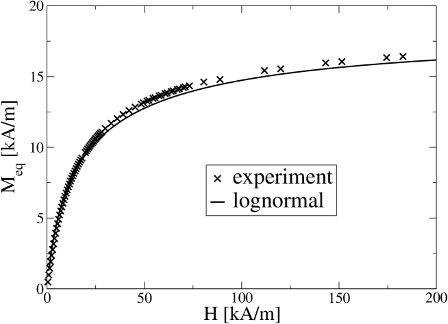
Figure 2: x: Experimental equilibrium magnetization $M_{eq}(H)$ used as input for the monodisperse calculations; full line: fit with lognormal contribution.

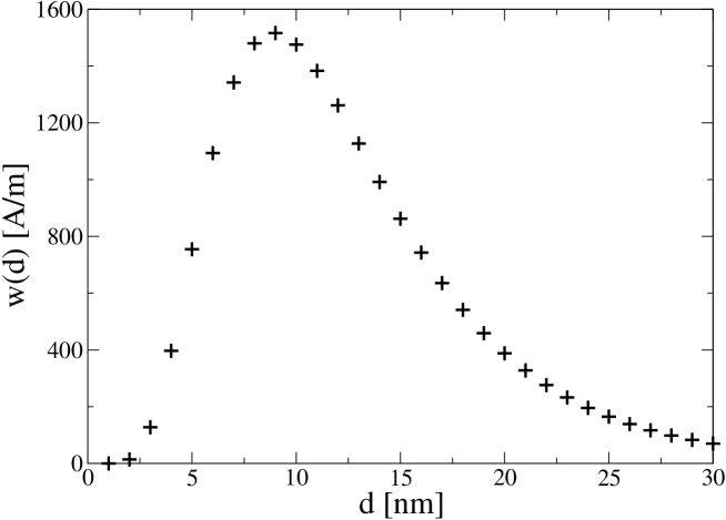
Figure 3: lognormal contribution $w(d_{i})$ ($d_{1}=1nm\dots d_{30}=30nm$) used as input for the polydisperse calculations.

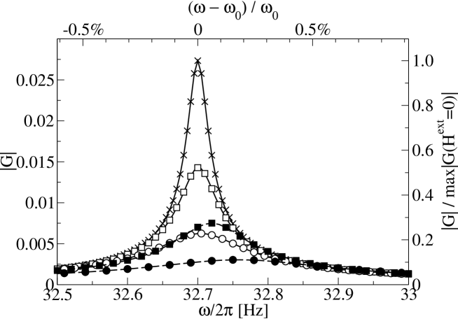
Figure 4: $|G|$ near the resonance $\omega_{0}$; x $H^{ext}=0kA/m$, squares $H^{ext}=5kA/m$, circles $H^{ext}=10kA/m$; filled symbols: polydisperse.

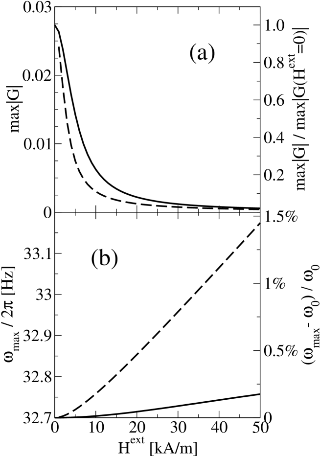
Figure 5: Maximum value $max|G|$ (a) and peak position $\omega_{max}$ (b) as a function of external field $H^{ext}$; full line monodisperse, dashed line polydisperse.

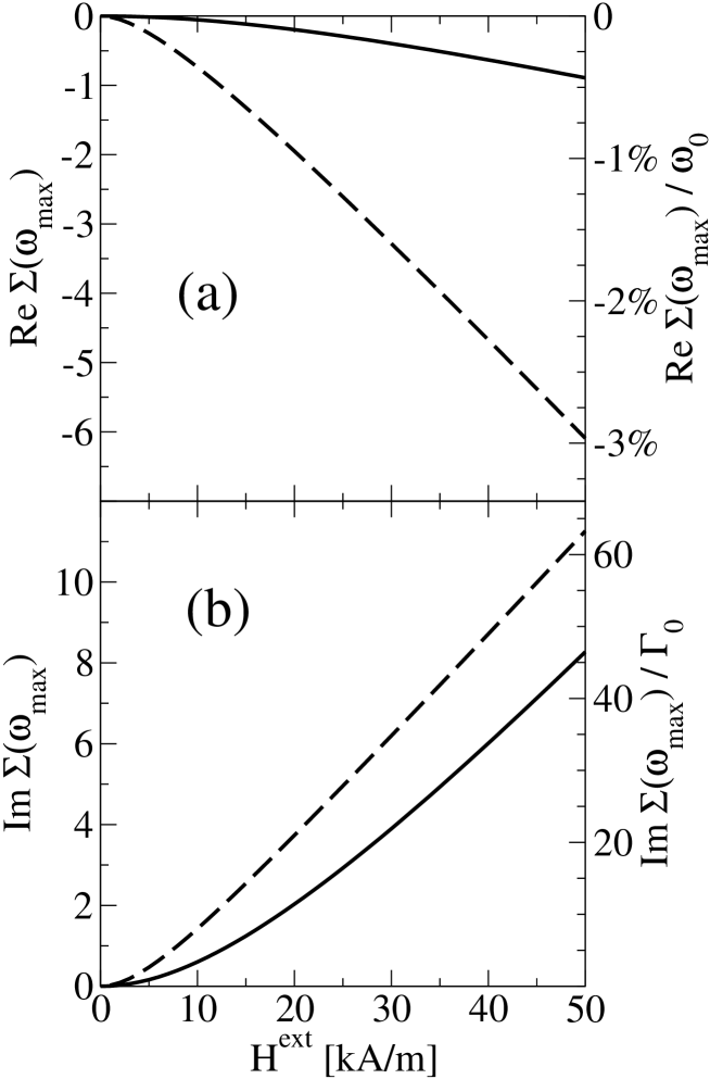
Figure 6: $Re(\Sigma)$ (a) and $Im(\Sigma)$ (b) at $\omega=\omega_{max}$; full line monodisperse, dashed line polydisperse.

- (1) R. E. Rosensweig, Ferrohydrodynamics, Cambridge University Press, Cambridge (1985).
- (2) J. Embs, H. W. Müller, C. E. Krill, F. Meyer, H. Natter, B. Müller, S. Wiegand, M. Lücke, R. Hempelmann, K. Knorr, Magnetohydrodynamics 37, 222 (2001).
- (3) J. Embs, H. W. Müller, M. Lücke and K. Knorr, Magnetohydrodynamics 36, 387 (2000); J. Embs, H. W. Müller, C. Wagner, K. Knorr and M. Lücke, Phys. Rev. E 61, R2196 (2000).