Scaling behavior of optimally structured catalytic microfluidic reactors

Abstract

In this study of catalytic microfluidic reactors we show that, when optimally structured, these reactors share underlying scaling properties. The scaling is predicted theoretically and verified numerically. Furthermore, we show how to increase the reaction rate significantly by distributing the active porous material within the reactor using a high-level implementation of topology optimization.

Chemical processes play a key role for the production and analysis of many substances and materials needed in industry and heath care. Generally, the optimization of these processes is an important goal, and with the introduction of microfluidic reactors involving laminar flows, the resulting concentration distributions mean better control and utilization of the reactors KiwiMinsker05a . These conditions make it possible to design reactors using the method of topology optimization SigmundBook , which recently has been applied to fluidic design of increasing complexity Borrvall:03a ; AGH-fluid ; Olesen:06a .

First, we report the finding of scaling properties of such optimal reactors. To illustrate the method we study a simple model of a chemical reactor, in which the desired product arises from a single first-order catalytic reaction due to a catalyst immobilized on a porous medium filling large regions of the reactor.

Next, we show that topology optimization can be employed to design optimal chemical micro-reactors. The goal of the optimization is to maximize the mean reaction rate of the micro-reactor by finding the optimal porosity distribution of the porous catalytic support. Despite the simplicity of the model, our work shows that topology optimization of the design of the porous support inside the reactor can increase the reaction rate significantly.

Our model system is a first-order catalytic reaction, $\mathrm{A}\stackrel{{\scriptstyle\mathrm{C}}}{{\longrightarrow}}\mathrm{B}$, taking place inside a microfluidic reactor of length $L$, containing a porous medium of spatially varying porosity $\gamma(\mathbf{r})$ and a buffer fluid filling the pores. The porosity $\gamma$ is defined as the local volume fraction occupied by the buffer fluid Desmet:03a , and it can vary continuously from zero to unity, where $\gamma=0$ is the limit of dense material (vanishingly small pores) and $\gamma=1$ is the limit of pure fluid (no porous material). The reactant A and the product B are dissolved with concentrations $a$ and $b$, respectively, in the buffer fluid, which is driven through the reactor by a constant, externally applied pressure difference $\Delta p$ between an inlet and outlet channel. The catalyst C is immobilized with concentration $c$ on the porous support.

The working principle of the reactor is quite simple. The buffer fluid carries the reactant A through the porous medium supporting the catalyst C. The reaction rate is high if at the same time the reactant A is supplied at a high rate and the amount of immobilized catalyst C is large. However, these two conditions are contradictory. For a given pressure drop $\Delta p$ the supply rate of A is high if $\gamma$ is high allowing for a large flow rate of the buffer fluid. Conversely, the amount of catalyst C is high if $\gamma$ is low corresponding to a dense porous support with a large active region. Consequently, an optimal design of the porous support must exist involving intermediate values of the porosity. Besides, the optimal design may involve an intricate distribution of porous support within the reactor, and to find this we employ the method of topology optimization in the implementation of Ref. Olesen:06a .

In the steady-state limit, the reaction kinetics is given by the following advection-diffusion-reaction equation for the reactant concentration $a$,

$$\big{[}\mathbf{u}(\gamma)\cdot\bm{\nabla}\big{]}a=D\bm{\nabla}^{2}a-k(\gamma)\,a.$$ (1)

Here $\mathbf{u}(\gamma)$ is the velocity field of the buffer fluid, $D$ is the diffusion constant of the reactant in the buffer, and $-k(\gamma)\,a$ is the reaction term of the first order isothermal reaction, which depends on the concentration of the catalyst C through $\gamma(\mathbf{r})$. In this problem three characteristic timescales $\tau_{A},\ \tau_{R}$ and $\tau_{D}$ naturally arise,

$$\tau_{A}=\frac{L}{u},\quad\tau_{D}=\frac{L^{2}}{D},\quad\tau_{R}=\frac{1}{k_{\Omega}},$$ (2)

which correspond directly to the advection, diffusion, and reaction term in Eq. (1), respectively. These time-scales will be used in the following theoretical analysis. Note that the index of $\Omega$ generally denote an average over the design region, e.g., $k_{\Omega}=\langle k(\gamma)\rangle_{\Omega}$.

The porosity field $\gamma(\mathbf{r})$ uniquely characterizes the reactor design since it determines both the distribution of the catalyst and the flow of the buffer. In the Navier–Stokes equation, governing the flow of the buffer, the presence of the porous support can be modelled by a Darcy damping force density $-\alpha(\gamma)\,\mathbf{u}$, where $\alpha$ is the local, porosity-dependent, inverse permeabilityBear72 . Assuming further that the buffer fluid is an incompressible liquid of density $\rho$ and dynamic viscosity $\eta$, the governing equations of the buffer in steady-state become

$$\rho(\mathbf{u}\cdot\bm{\nabla})\mathbf{u} =-\bm{\nabla}p+\eta\nabla^{2}\mathbf{u}-\alpha(\gamma)\,\mathbf{u},$$ (3a)

$$\bm{\nabla}\cdot\mathbf{u} =0.$$ (3b)

The coupling between $\alpha$ and $\gamma$ is given by the function $\alpha(\gamma)\equiv\alpha_{\max}\,\frac{q(1-\gamma)}{q+\gamma}$, where $\alpha_{\max}$ is determined by the non-dimensional Darcy number $Da=\frac{\eta}{\alpha_{\max}\,L^{2}}$, and $q$ is a positive parameter used to ensure global convergence of the topology optimization methodBorrvall:03a ; Olesen:06a . In this work $Da$ is typically around $10^{-5}$, resulting in a strong damping of the buffer flow inside the porous support. The model is solved for a given $\gamma(\mathbf{r})$ by first finding $\mathbf{u}(\gamma)$ from Eqs. (3a) and (3b) and then $a(\mathbf{r})$ from Eq. (1).

Our aim is to optimize the average reaction-rate $(k(\gamma)\,a)_{\Omega}$ of the reactor by finding the optimal porosity field $\gamma(\mathbf{r})$. We therefore introduce the following objective function $\Phi(\gamma)$, which by convention has to be minimized,

$$\Phi(\gamma)=-(k(\gamma)\,a)_{\Omega}.$$ (4)

To better characterize the performance of the reactor and to introduce the related quantities, we first analyze a simple 1D model defined on the $x$-axis. The porous medium is placed in the reaction region $\Omega$ extending from $x=0$ to $x=L$. Eq. (3b) leads to a constant flow velocity $u$, and as the complete pressure-drop occurs in the porous medium, we have $p(0)=p_{0}+\Delta p$ and $p(L)=p_{0}$. In this case the boundary conditions for the advection-diffusion-reaction equation Eq. (1) are $a(-\infty)=a_{0}$, $a^{\prime}(-\infty)=0$, and $a^{\prime}(\infty)=0$, where the primes indicate $x$-derivatives. We denote the outlet concentration $a(\infty)=a_{L}$. From Eqs. (1) and (4), we then derive the following expression of the objective function

$$\Phi(\gamma) =-\langle k(\gamma)\,a\rangle=\frac{1}{L}\int_{0}^{L}\!\!\left[u(\gamma)a^{\prime}-D\,a^{\prime\prime}\right]dx$$

$$=\frac{u(\gamma)}{L}\left(a_{L}-a_{0}\right)-\frac{D}{L}\big{[}a^{\prime}(L)-a^{\prime}(0)\big{]}.$$ (5)

For simplicity, we now limit the analysis to the non-diffusive case ($D=0$), and from Eq. (5) we get the objective function defined in terns of the reaction conversion $\mathcal{C}$,

$$\Phi(\gamma)=-\frac{u(\gamma)\,a_{0}}{L}\,\mathcal{C},\quad\mathrm{with}\quad\mathcal{C}\equiv 1-\frac{a_{L}}{a_{0}}.$$ (6)

With an explicit $x$ dependence of the reaction rate coefficient $k(x)$, we obtain $u(\gamma)a^{\prime}=-k(x)\,a$ with the solution

$$a(x)=a_{0}\,e^{-\frac{K(x)}{u(\gamma)}},\quad\mathrm{with}\quad K(x)\equiv\int_{0}^{x}k(\tilde{x})d\tilde{x}.$$ (7)

This leads to the following expression of the conversion:

$$\mathcal{C}=1-e^{-\frac{K(L)}{u(\gamma)}}=1-e^{-\frac{k_{\Omega}}{u(\gamma)}L}=1-e^{-\delta},$$ (8)

where we have introduced the dimensional-less Damköhler number $\delta$ Damkohler:1937

$$\delta\equiv\frac{\tau_{A}}{\tau_{R}}=\frac{k_{\Omega}}{u(\gamma)}L,$$ (9)

having the physical interpretation of the ratio between the advection and the reaction timescale.

To derive the flow speed $u(\gamma)$ in the 1D model we first let $q\rightarrow\infty$ resulting in $\alpha(\gamma)=\alpha_{\max}(1-\gamma)$ and then by integrating Eq. (3a), $0=-p^{\prime}-\alpha_{\max}(1-\gamma)\,u$, we get

$$u=\frac{\Delta p}{\alpha_{\max}(1-\gamma_{\Omega})L}=\frac{Da}{1-\gamma_{\Omega}}\,\frac{\Delta p\,L}{\eta}.$$ (10)

To solve the 1D optimization problem analytically, we chose to abandon the spatial variations of $\gamma$ in the 1D model. We have to find the solutions to $\frac{\partial\Phi}{\partial\gamma_{\Omega}}\equiv 0$, and from Eqs. (6) and (8), we end up by having to solve the following equation

$$1-e^{\delta}+\delta(1+\beta)=0,$$ (11)

where we have assumed that $k(\gamma_{\Omega})\propto(1-\gamma_{\Omega})^{\beta}$. The specific properties of the catalytic reaction determines the value of $\beta$, e.g., if the full volume of the porous medium is active then $\beta=1$, while if only the surface is active then $\beta=2/3$. Solving Eq. (11) gives the optimal value of $\delta_{\beta}$, where the reference to $\beta$ now is explicit.

All numerical solutions are found using the commercial numerical modelling-tools MatlabMATLAB and COMSOL COMSOL . To validate numerically the analytic results of the 1D model, we solve Eqs. (1) and (10) for a given homogeneous design variable $\gamma_{\Omega}$ and find the optimal value using a brute-force optimization method MATLABOptim .

To obtain a general scaling parameter for the problem defined in Eq. (1) we reintroduce diffusion. However, to minimize the trivial influence from the inlet and outlet, we only study the limit of low diffusion, e.g., $\tau_{D}\gg\tau_{A},\tau_{R}$. In this limit the optimal reactors involve a balance between the advection and reaction processes, and consequently we expect that $\tau_{A}$ and $\tau_{R}$, should enter on equal footing in the scaling parameter. We are therefore led to propose the following dimensional-less form of the scaling-parameter

$$\frac{\sqrt{\tau_{A}\,\tau_{R}}}{\tau_{D}}=\frac{D}{\sqrt{k(\gamma_{\Omega})\,u(\gamma_{\Omega})\,L^{3}}}.$$ (12)

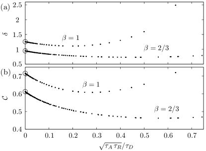
Figure 1: Plot of 1D results showing (a) Damköhler number $\delta$ and (b) conversion $\mathcal{C}$, both as a function of $\sqrt{\tau_{A}\,\tau_{R}}/\tau_{D}$ and for optimal choices of porosity. In both cases $\beta=2/3,\,1$ and the parameter-scan of each choice consist of 512 optimizationsParamScan which collapse nicely. For zero difffusion, $\sqrt{\tau_{A}\,\tau_{R}}/\tau_{D}=0$, Eqs. (11) and (8) give the exact results $\delta_{2/3}=0.9474$, $\delta_{1}=1.2564$, $\mathcal{C}_{2/3}=0.6122$, and $\mathcal{C}_{1}=0.7153$, which are marked by circles on the ordinate axis.

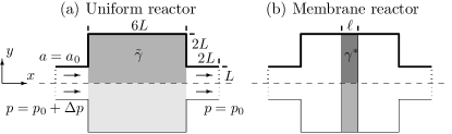
Figure 2: Illustration of the two simple 2D reactor setups, (a) the uniform reactor with porosity $\tilde{\gamma}$ and (b) the membrane reactor of width $\ell$ and with porosity $\gamma^{\ast}\equiv 0$. The horizontal dashed line is a symmetry-line.

Figure 1 shows that the measured values of $\delta_{\beta}$ and $\mathcal{C}_{\beta}$ for optimal porosity both scale with respect to $\sqrt{\tau_{A}\,\tau_{R}}/\tau_{D}$. The simulations cover 512 optimal reactors in a wide and dense parameter-scan ParamScan , and as they collapse almost perfectly on single curves, we have not distinguished the data-points further. In the non-diffusive case $D=0$ and $\sqrt{\tau_{A}\,\tau_{R}}/\tau_{D}=0$, exact values of $\delta_{\beta}$ and $\mathcal{C}_{\beta}$ are determined by Eqs. (8) and (11), and they match exactly with the numerical results, as seen in Fig. 1, where they are marked by circles on the ordinate.

We now introduce three types of 2D reactors: the uniform reactors, Fig. 2(a), the membrane reactors, Fig. 2(b), and the topology optimized reactors, for which a few is shown in Fig. 3. First we optimize the simple reactors in Fig. 2. They both depend only on one variable, which for the uniform reactor is the uniform porosity $\tilde{\gamma}$, and for the membrane reactor is the width $\ell$ of a porous membrane of porosity $\gamma^{\ast}\equiv 0$ MATLABOptim . Because of mirror-symmetry in the $xz$-plane, only the upper half of the reactors are solved in all the following work.

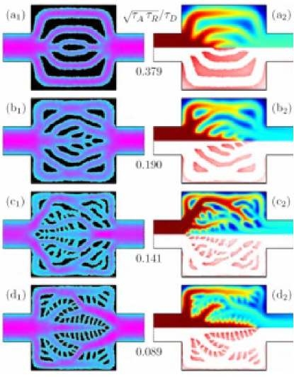
Figure 3: Representative collection of topology optimized reactor designs for deceasing values of $\sqrt{\tau_{A}\,\tau_{R}}/\tau_{D}$. (Left column) The distribution $\gamma$ of porous material in black together with a color-grading indication of the flow speed $u$. (Right column) The concentration $a$ on top with the reaction rate $k(\gamma)a$ below. Parameters (in SI units) $L=10^{-3}$ and the following values of $[Da,\,D,\,\Delta p,\,k_{a}]$: (a) $[10^{-4},\,3\times 10^{-8},\,0.25,\,0.25]$, (b) $[10^{-4},\,3\times 10^{-8},\,0.25,\,1]$, (c) $[10^{-5},\,10^{-8},\,0.5,\,1]$, and (d) $[10^{-4},\,10^{-8},\,0.25,\,0.5]$.

In the third type of 2D reactors we let the porosity $\gamma(\mathbf{r})$ vary freely within the same design region as for the uniform reactor. The optimal design is found using the topology optimization method, described in detail in Ref. Olesen:06a . This is an iterative method, in which, starting from an initial guess $\gamma_{0}$ of the design variable, the $n$th iteration consists of first solving the systems for the given design variable $\gamma_{n}$, then evaluating the sensitivities $\frac{\partial\Phi}{\partial\gamma}$ by solving a corresponding adjoint problem, and finally obtaining an improved updated $\gamma_{n+1}$ by use of the ”method of moving asymptotes” (MMA)MMA ; MMAprogram . In Fig. 3 is shown a representative collection of topology optimized designs together with the corresponding flow speed $u$, concentration $a$, reaction rate $k(\gamma)a$, and parameter values. In the large parameter space under investigation, our work shows a systematic decrease of pore-sizes and the emergence of finer structures in the topology optimized reactors as the scaling parameter $\sqrt{\tau_{A}\,\tau_{R}}/\tau_{D}$ is decreased.

In Fig. 4 the conversion $\mathcal{C}$ is plotted as a function of $\sqrt{\tau_{A}\,\tau_{R}}/\tau_{D}$ for all optimal reactors of this work. It shows that all reactors collapse on curves similar to the 1D reactors, although the topology optimized reactors exhibit a larger spread. We believe that this scaling is a signature of a general property of optimal immobilized catalytic reactors. Note that the conversion of the uniform reactor in the low diffusion limit is a few percent higher than the theoretical estimate, an effect caused by low convection in the corners, resulting in ’dead zones’.

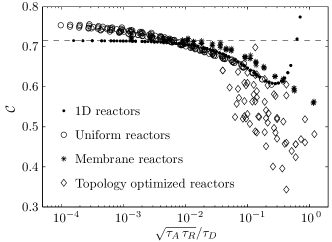
Figure 4: Overall scaling of the conversion $\mathcal{C}$ as a function of $\sqrt{\tau_{A}\,\tau_{R}}/\tau_{D}$ for the different optimal reactors. The abscissa is logarithmic to emphasize the common scaling behavior. The dashed line indicate the theoretical value $\mathcal{C}_{1}$ for zero diffusion in the 1D case.

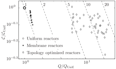
Figure 5: Log-log plot of the relation between convection $\mathcal{C}$ and flow rate $Q$ for the different reactors, when normalized with values $\mathcal{C}_{\mathrm{unif}}$ and $Q_{\mathrm{unif}}$ of the uniform reactors. The reaction rate improvements are shown at the top (see text).

In terms of the objective function $\Phi$ the topologically optimized reactors are significant improved compared to the simple 2D reactors. To investigate the nature behind this improvement, we show in Fig. 5 a log-log plot of the flow rate $Q$ and the conversion $\mathcal{C}$ normalized by the values $\mathcal{C}_{\mathrm{unif}}$ and $Q_{\mathrm{unif}}$ of the uniform reactors at the same parameters. Because Eq. (6) gives the following scaling of the objective function $\Phi\sim Q\,\mathcal{C}$, the rate of improvement with respect to the uniform reactors can be read off directly, as the contours of the improvement-factors of $\Phi$ become straight lines, as showed by the dashed lines labelled by the corresponding factors in Fig. 5. It is seen that topology optimization can increase the reaction rate of the optimal reactors by nearly a factor 20, and furthermore it does so by increasing the flow rate at the expense of lower conversions. The important insight thus gained is that the distribution of the advected reactant by the microfluidic channel network over a large area at minimal pressure-loss plays a significant role when optimizing microreactors.

To conclude, we have analyzed a single first-order catalytic reaction in a laminar microfluidic reactor with optimal distribution of porous catalyst. The flow is pressure-driven and the flow through the porous medium is modelled using a simple Darcy damping force. Our goal has solely been to optimize the average reaction rate, with no constrains on the conversion or the catalytic properties. A characterization of the optimal configuration has been derived theoretically and validated numerically. It shows an general scaling behavior, depending only on the reaction properties of the catalyst. The analysis is based on a very simple reaction since this emphasizes the points that the optimization of even simple reactions result in to non-trivial scaling properties and complex optimal designs. Using topology optimization to design optimal reactors give rise to reaction rate improvements of close to a factor 20, compared to an corresponding optimal uniform reactor, and the improvement originates mainly due to an improved transport and distribution of the reactant. Furthermore, for the topology optimized reactors, we have found a systematic decrease of pore-sizes and the emergence of finer structures as the scaling parameter is decreased. Our work points out a new, general, and potentially very powerful method of improving microfluidic reactors.

F. O. was supported by The Danish Technical Research Council No. 26-03-0037 and No. 26-03-0073.

References

- (1) L. Kiwi-Minsker and A. Renken, Catalysis Today 110, 2 (2005).
- (2) M. P. Bendsøe and O. Sigmund, Topology Optimization-Theory, Methods and Applications (Springer, Berlin 2003).
- (3) T. Borrvall and J. Petersson, Int. J. Num. Meth. Fluids 41, 77 (2003).
- (4) A. Gersborg-Hansen, O. Sigmund and R. B. Haber, Structural and Multidisciplinary Optim. 30, 181 (2005).
- (5) L. H. Olesen, F. Okkels, and H. Bruus, Int. J. Num. Meth. Eng. 65, 975 (2006).
- (6) G. Desmet, J. D. Greef, H. Verelst, and G. V. Baron, Chem. Eng. Sci. 58, 3187 (2003).
- (7) J. Bear, Dynamics of Fluids in Porous Media (Am. Elsevier Publ. Com., New York 1972).
- (8) G. Damköhler, Chem - Ing. Tech. 3, 359 (1937).
- (9) The MathWorks, Inc. (www.mathworks.com).
- (10) COMSOL AB (www.comsol.com).
- (11) The Matlabroutine fminbnd minimizes a single variable using a golden section search and parabolic interpolation.
- (12) Parameter-scan: with , and , .
- (13) K. Svanberg, Int. J. Num. Meth. Eng. 24, 359 (1987).
- (14) A MATLAB implementation, mmasub, of the MMA optimization algorithm MMA can be obtained (free of charge for academic purposes) from Krister Svanberg, KTH, Sweden. E-mail: krille@math.kth.se