Stochastic model for market stocks with strong resistances

Javier Villarroel

Univ. de Salamanca, Fac. de Ciencias,

Plaza Merced s/n, Salamanca 37008, Spain

(Javier@usal.es)

Keywords.

Option and derivative pricing, Econophysics, Stochastic differential equations.

PACS

0.7.05 Mh, 89.65.Gh, 02.50.Ey, 05.40.Jc,

Abstract.

We present a model to describe the stochastic evolution of stocks that show a strong resistance at some level and generalize to this situation the evolution based upon geometric Brownian motion. If volatility and drift are related in a certain way we show that our model can be integrated in an exact way. The related problem of how to prize general securities that pay dividends at a continuous rate and earn a terminal payoff at maturity $T$ is solved via the martingale probability approach.

1 Introduction

We consider an ideal model of financial market consisting of two securities: a savings account $Z_{t}$ evolving via $dZ_{t}=r_{t}Z_{t}dt$, where $r_{t}$ is the instantaneous interest rate of the market and is assumed to be deterministic (but not necessarily constant); and a ”risky” asset whose price at time $t$: $X_{t}$, evolves according to some stochastic differential eq. (SDE) driven by Brownian motion (BM). As it is well known, the prototype model for stocks-price evolution assumes that the return process $R_{t}=\log X_{t}$ follows a random walk or BM with drift and hence that prices $X_{t}$ evolve via the popular geometric Brownian motion (GBM) model, i.e., that $X_{t}$ satisfies

$$dX_{t}=\mu X_{t}dt+\sigma X_{t}dW_{t}$$

Here $\mu$ is the mean return rate and $\sigma$ the volatility which are supposed to be constants while $W_{t}$ is a Brownian motion under the empirical or real world probability. We remark that here and elsewhere in this article integrals and SDE’s are understood in the sense of Itô’s calculus. Transition to standard (Stratonovitch) calculus can be done if wished.

The solution to this SDE is given by

$$X_{t}^{\text{GBM}}=x_{0}\exp\Big{\{}\sigma W_{t}+\left(\mu-\frac{\sigma^{2}}{2}\right)t\Big{\}}$$

After the seminal work of Black and Scholes [1] and Merton [2], who derive a formula to price options on stocks with underlying dynamics based upon GMB, eq. (1) has become the paradigmatic model to describe both price evolution and derivatives pricing. However, while such a simple model captures well the basic features of prices it does not quite account for more stylized facts that empirical prices show; among them we mention the appearance of ”heavy tails” for long values of the relevant density probability distributions of returns [3,4]; further, the empirical distribution shows an exponential form for moderate values of the returns, which is not quite fitted by the predicted log-normal density implied by (2). The existence of self-scaling and long memory effects was first noticed in [5]. Due to all this option pricing under this GBM framework can not fully account for the observed market option prices and the classical Black-Scholes $\&$ Merton (BSM) formula is found to overprice (respectively underprice) ”in (respectively, out of) the money options”. Apparently, for empirical prices of call options to fit this formula an extra dependence in the strike price, the volatility smile, must be introduced by hand.

After the seminal paper by Mantegna and Stanley who studied the empirical evolution of the stock index S$\&$P500 of the American Stock Exchange during a five year period, several authors have elaborated on the possibility that price dynamics involves Levy process and have discussed option pricing in such a framework (See [5-13]). For complete accounts of option pricing and stochastic calculus from the economist and, respectively, physicist, points of view see [14-17] and [18-21].

Here we shall focus in another different aspect that some traded stocks seem to present, viz the possibility of having, at some level, strong resistances both from above or below. For example, corporations or major institutions may have laid out a policy under which heavy buy orders are triggered whenever the stock price hits this level. Such feature can not be described with Eq. (1) as under such an evolution prices can reach any value in $(0,\infty)$. Concretely, in this paper we want to model the evolution of a market stock which has a strong lower resistance at some level $c$ where we suppose that $c$ is a constant.

In section (2) we present a model that incorporates an attainable barrier at the point $x=c>0$ and hence can, in principle, be used to account for such a fact. We next derive the evolution of the asset and the probability distribution function. It turns out that $c$ is a regular barrier in terms of Feller’s boundary theory and hence a prescription on how to proceed once reached must be given. In section (3) we study pricing of securities under such a model and obtain a closed formula for valuation of European derivatives that have, in addition, a continuous stream of payments. We tackle this problem using the Martingale formalism of Harrison et al [22] and obtain the partial differential equation (PDE) that the price of a security satisfies. Solving this eq. corresponding to particular final conditions we obtain the price of options under this model. This price is compared with that given by the standard Black$\&$ Scholes- Merton formula. In the appendix we consider some technical issues concerning value of the market price of risk and the the existence of the martingale measure or risk free probability under which securities are priced.

2 Price evolution under the martingale probability

Let $r_{t}$ be the deterministic interest rate at time $t$ and $Z_{t}=\exp\int_{0}^{t}r_{s}ds$ be a ”savings account ”. As we pointed out we consider that $X_{t}$ is the $t$-price of a tradeable asset that has a strong lower resistance at some constant level $c$ where $0<c<x_{0}\equiv X_{0}$. Mathematically this implies that the values of $X_{t}$ must be restricted to the interval $[c,\infty)$ and hence $X_{t}$ must have a boundary point of a certain kind at $x=c$. From intuitive financial arguments the boundary can not be of absorbing type since in that case, once reached, the price $X_{t}$ remains there. Further it seems reasonable to assume that there exists positive probability to attain the boundary; we suppose that this event ”triggers” bid orders and hence that $X_{t}$ ricochets upon hitting the boundary. Therefore in such situation the assumption that prices evolve via Eq. (1) is no longer valid. The obvious modification wherein prices evolve as

$$\tilde{X}_{t}^{\text{GBM}}\equiv c+(x_{0}-c)e^{\sigma W_{t}+\left(\mu-\frac{\sigma^{2}}{2}\right)t}$$

is also ruled out as this evolution implies that $c<X_{t}<\infty$ but the value $X_{t}=c$ is never attained and the probability to get arbitrarily close to the barrier tends to zero with the distance to it. Thus trajectories corresponding to a such model never quite seem to reach the support(In terms of Feller’s theory briefly reminded below $x=c$ is a natural barrier at which Feller functions blow up).

Motivated by similar ideas in the context of the Cox-Ingersoll-Ross model of interest rate dynamics [23] we now introduce a more satisfactory model which satisfies the aforementioned features and is at the same time analytically tractable; we shall suppose that $X_{t}$ evolves via the SDE

$$dX_{t}=a(t,X_{t})dt+b(t,X_{t})dW_{t},\text{ where }a(t,x)=\mu x,~{}~{}b(t,x)=\sigma(t)\sqrt{x^{2}-c^{2}}$$

Here $X_{0}=x_{0}>c$, $\mu$ is the stock mean rate of return and $b(t,x)$ the volatility coefficient. Indeed, under such a dynamics it follows from (4) that as $x$ approaches the point $c$, $b(t,x)$ tends to zero and hence $X_{t}$ evolves roughly like $dX_{t}=\mu X_{t}dt$ implying that $X_{t}$ will increase and then escape from the boundary.

For valuation purposes one needs to consider the evolution under a new probability that might be different to the empirical observed probability. Mathematically speaking a such a probability is defined requiring that under it the discounted prices $X^{\prime}_{t}\equiv X_{t}/Z_{t}$ are martingales (this risk-neutral probability was introduced in [22] although the underlying idea pervades the original work of Black-Scholes $\&$ Merton [1,2]). Stated another way, this means that under the risk-neutral probability, the stock price $X_{t}$ evolves, on average, as the riskless security $Z_{t}$ thereby preventing arbitrage opportunities. Indeed, the martingale property implies

$$e^{-\int_{0}^{t}r_{s}ds}\mathbb{E}^{*}\Big{(}X_{t}\Big{|}X_{0}\Big{)}=\mathbb{E}^{*}\Big{(}X^{\prime}_{t}\Big{|}X_{0}\Big{)}=\mathbb{E}^{*}\Big{(}X^{\prime}_{t}\Big{|}X^{\prime}_{0}\Big{)}=X^{\prime}_{0}=x_{0}$$

where $\mathbb{E}^{*}\Big{(}X_{t}\Big{|}X_{0}\Big{)}$ is the conditional average of $X_{t}$ given $X_{0}$ with respect to the martingale probability. Hence

$$\mathbb{E}^{*}\Big{(}X_{t}\Big{|}X_{0}\Big{)}=x_{0}Z_{t}$$

More generally, given the past history $\mathcal{F}_{s}$ of the process up to time $s$ (i.e., the $\sigma$-field of past events) one has

$$\mathbb{E}^{*}\Big{(}X_{t}\Big{|}\mathcal{F}_{s}\Big{)}=Z_{t}\mathbb{E}^{*}\Big{(}X^{\prime}_{t}\Big{|}\mathcal{F}_{s}\Big{)}=Z_{t}X^{\prime}_{s}\equiv X_{s}e^{\int_{s}^{t}r_{l}dl}$$

We shall assume that our market is efficient, i.e., that the martingale probability $\mathbb{P}^{*}$ exists– which is not always the case. In such a case the explicit form of the original drift coefficient is only needed to go back to the empirical or real world probabilities. Indeed, it follows from these arguments that consideration of this probability amounts to redefining the evolution equation without changing the volatility coefficient $b(t,x)$ but replacing the drift coefficient to $a^{*}(t,x)=r_{t}x$, independent of the initial coefficient $a(t,x)\equiv\mu x$.

Unfortunately, in general it is not possible to solve the redefined SDE corresponding to the diffusion coefficients (4) with $a^{*}(t,x)=r_{t}x$. However, it turns out that in the particular case when $\sigma^{2}(t)=2r(t)$, i.e., for eq. (8) below, then both this SDE and the prizing problem can be solved as we next show. We shall consider this case and hence we suppose that under the risk neutral probability $\mathbb{P}^{*}$, $X_{t}$ evolves via the SDE

$$dX_{t}=r_{t}X_{t}dt+\sqrt{2r_{t}\big{(}X_{t}^{2}-c^{2}\big{)}}dW_{t}^{*},~{}~{}X_{0}=x_{0}>c$$

Here $W_{t}^{*}$ is a BM with respect to the risk neutral probability. Technically, the existence and nature of all objects introduced below is a difficult point. In the appendix we sketch how to perform such a construction.

In the sequel all quantities are referred to the probability $\mathbb{P}^{*}$ and hence $X_{t}$ evolves via (8) which is our fundamental equation. Further for ease of notation we drop here and elsewhere the use of ^∗.

The return process $R_{t}\equiv\log X_{t}/x_{0}$ is found via Itô’s rule to satisfy

$$dR_{t}=r_{t}c^{2}e^{-2R_{t}}dt+\sqrt{2r_{t}\Big{(}1-c^{2}e^{-2R_{t}}\Big{)}}dW_{t},~{}~{}R_{0}=0$$

Thus only when $R_{t}$ is close to $0$ it does behave like a classical random walk.

Useful information about the behavior of the price process at $x=c$ follows by careful inspection of the nature of the boundary $x=c$. Consider the Feller functions $\Sigma(c,x),\Omega(c,x)$ defined by

$$\Sigma(c,x)=\int_{c}^{x}\frac{p(z)}{b^{2}(z)}dz\int_{c}^{z}{dy\over p(y)};~{}\Omega(c,x)=\int_{c}^{x}\frac{dy}{p(y)}\int_{c}^{y}{p(z)\over b^{2}(z)}dz.$$

where $p(x)\equiv\sqrt{x^{2}-c^{2}}$. The reader is referred for these matters to [24]. Notice that the integrand is singular since it has a square root singularity at $x=c$. Upon evaluation of the integrals we find that

$$\Sigma(c,x)=\Omega(c,x)=\frac{1}{4r}\log^{2}\big{(}{x+\sqrt{x^{2}-c^{2}}\over c}\big{)}$$

Thus, unlike what happens in the model defined by (3), we have that $\Sigma(c,x)=\Omega(c,x)<\infty$ are finite, corresponding to a regular boundary which can be both reached and exited from in finite time with positive probability.

While Feller analysis shows that the boundary is attainable it does not clarify if the process can be continued past the boundary (and hence whether prices below the level $x=c$ can be attained). Further it it is unclear what is the probability to reach the boundary or how the to continue the process upon hitting the boundary.

These kind of problems regarding behavior of the process at and past the boundary are generically quite difficult to tackle. It turns out that for our particular model the behavior of the process is completely determined. Actually we have found that the solution to eq. (8) is given in a fully explicit way by

$$X_{t}=c\cosh\big{(}\int_{0}^{t}\sqrt{2r_{s}}dW_{s}+\kappa\Big{)}$$

where $\kappa\equiv\cosh^{-1}(x_{0}/c)$. A typical path $t\to X_{t}$ is shown below in Fig. 1. To prove (12) let $\tilde{X}_{t}\equiv g(Y_{t})$ where

$$g(z)=c\cosh\big{(}z),~{}Y_{t}\equiv\kappa+\int_{0}^{t}\sqrt{2r_{s}}dW_{s}$$

Using Itô’s rule and the fact that $dY_{t}=\sqrt{2r_{t}}dW_{t}$ we find that $\tilde{X}_{t}$ has diffusion coefficients $\tilde{a}(t,x),\tilde{b}(t,x)$ satisfying at $x=g(z)$

$$\tilde{a}(t,x)={2r_{t}\over 2}\partial_{zz}g=r_{t}g(z)\equiv r_{t}x$$

$$\tilde{b}(t,x)=\sqrt{2r_{t}}\partial_{z}g=\sqrt{2r_{t}}c\sinh\big{(}z)=\sqrt{2r_{t}\Big{(}x^{2}-c^{2}\Big{)}}$$

i.e. $\tilde{X}_{t}\equiv g(Y_{t})$ solves the SDE (8).

Notice that the last equality and the fact that the $\sinh$ takes both signs, imply that the following prescription must be given at the barrier:

$$b\big{(}g(z)\big{)}=-b\big{(}g(-z)\big{)}$$

Thus (12) solves (8) provided the square root is defined with a branch cut on $(c,\infty)$.

We note that the conditional density $f(s,Y|t,y),t<s$ of $Y_{t}$ solves

$$\Big{(}\partial_{t}+r(t)\partial_{yy}\Big{)}f=0;f(s,y|s,y_{0})=\delta(y-y_{0})$$

which is converted into the classical BM or heat equation upon time transformation via $t^{\prime}=\varphi(t)$ where we define

$$\varphi(q,r)\equiv 2\int_{q}^{r}r_{s}ds;\varphi(t)\equiv\varphi(0,t)\equiv 2\int_{0}^{t}r_{s}ds$$

It follows that the process $Y_{t}$ has the distribution of a BM evaluated at time $t^{\prime}$ and hence we can represent $X_{t}$ as

$$X_{t}=c\cosh Y_{t}\text{ where }Y_{t}=\kappa+B_{\varphi(t)}$$

and $B_{t}$ is a new BM. It follows from (12) that $X_{t}\geq c$ and that $X_{t}$ attains the barrier $c$ whenever the process $Y_{t}$ reaches $0$ , i.e., when $\int_{0}^{t}\sqrt{2r_{s}}dW_{s}+\kappa=0$, which, according to (18) happens eventually with probability one. As pointed out, it follows from (18) that in that case the process $X_{t}$ is reflected and hence the level $x=c>0$ acts as a resistance of the stock value.

Let us now obtain $p(T,X|t,x)$, the probability density function (pdf) of the price process conditional on the value at time $t$: $X_{t}=x,t<T$. This pdf satisfies the backwards Kolmogorov-Fokker-Planck equation

$$\Big{(}\partial_{t}+r(t)(x^{2}-c^{2})\partial_{xx}+rx\partial_{x}\Big{)}p=0;p(T,X|T,x)=\delta(x-X)$$

Motivated by (13,17) above we define new coordinates $t^{\prime}=\varphi(t),y=\log\Big{(}x+\sqrt{x^{2}-c^{2}}\Big{)}-\log c$. In terms of the new coordinates $p$ solves

$$\Big{(}\partial_{t}+{1\over 2}\partial_{yy}\Big{)}p=0;p(T,Y|T,y)=\delta(c\cosh y-c\cosh Y)$$

Using the well known formula

$$c\delta(c\cosh y-c\cosh Y)=\Big{(}\delta(y-Y)+\delta(y+Y)\Big{)}/|\sinh Y|$$

we find that

$$p(T,X|t,x)={1\over\sqrt{2r_{t}\big{(}X^{2}-c^{2}\big{)}}}\underset{\pm}{\sum}\exp\Big{(}-{1\over 2\varphi(t,T)}\log^{2}{x+\sqrt{x^{2}-c^{2}}\over X\pm\sqrt{X^{2}-c^{2}}}\Big{)}$$

We next compare the evolution of prices under this model and that described by GBM. For a meaningful comparison we need to have $r_{t}=r$ constant and, in Eq. (1), $\mu\equiv r,\sigma=\sqrt{2r}$. In this case (2) yields

$$X_{t}^{\text{GBM}}=x_{0}e^{\sqrt{2r}W_{t}}$$

Note that whenever $W_{t}>>1$ both process behave in a very similar way:

$$\underset{W_{t}\to\infty}{\lim}X_{t}/X_{t}^{\text{GBM}}={x_{0}+\sqrt{x_{0}^{2}-c^{2}}\over 2x_{0}}$$

However as $W_{t}\to-\infty$ then

$$X_{t}\approx\big{(}x_{0}-\sqrt{x_{0}^{2}-c^{2}}\big{)}/2e^{\sqrt{2}r|W_{t}|}\to\infty,X_{t}^{\text{GBM}}=x_{0}e^{\sqrt{2}rW_{t}}\to 0$$

Finally, we note that in the limit $c\to 0$ we can recover (2) from (18). A careful calculation shows that

$$\underset{c\to 0}{\lim}X_{t}=x_{0}\exp B_{2rt}$$

and hence, using that $\sqrt{2r}W_{t}$ is a BM at time $2rt$, we recover (2).

3 valuation of securities

We consider here the valuation of securities earning a terminal payoff $\Theta_{1}(X_{T})$ at maturity $T$. We also allow for the security to pay dividends at a continuous rate $\Theta_{2}(s,X_{s}),t\leq s\leq T$ where we suppose that both $\Theta_{1}:\mathbb{R}\to\mathbb{R}$ and $\Theta_{2}:\mathbb{R}^{+}\times\mathbb{R}\to\mathbb{R}$ are continuous. The standard case of stock option valuation corresponds to taking $\Theta_{1}(x)=(x-k)^{+},\Theta_{2}(x)=0$ where $k$ is the strike.

Let $v_{t}$ be the (actual) $t$-price of such European derivative maturing at $T$, which must also depend on $T$ and the actual price $x=X_{t}$ of the stock.

We assume the existence of risk-neutral probability $\mathbb{P}^{*}$ under which relative prices of stocks and more generally, of self-financing strategies $v^{\prime}_{t}\equiv v_{t}/Z_{t}$ are martingales with respect to the history of the process up to time $t$: $\mathcal{F}_{t}$ (notice that we shall drop again the symbol^∗). If this is the case, reasoning similarly as in (7) and use of the martingale property yields that

$$v_{t}e^{\int_{t}^{T}r_{l}dl}\equiv Z_{T}v^{\prime}_{t}=Z_{T}\mathbb{E}\Big{(}v^{\prime}_{T}\Big{|}\mathcal{F}_{t}\Big{)}=\mathbb{E}\Big{(}v_{T}\Big{|}\mathcal{F}_{t}\Big{)}$$

To continue further we note that $v_{t}$ must satisfy at $t=T$ that

$$v_{T}=\Theta_{1}(X_{T})+\int_{t}^{T}\Theta_{2}(s,X_{s})Z_{T}/Z_{s}ds\equiv v_{T}^{1}+v_{T}^{2}$$

as the RHS is precisely the earning at maturity. Note further that $v_{T}^{1}\equiv\Theta_{1}(X_{T})$ is obviously Markovian and hence that $\mathbb{E}\Big{(}v_{T}\Big{|}\mathcal{F}_{t}\Big{)}=\mathbb{E}\Big{(}v_{T}\Big{|}X_{t}\Big{)}$.

It can be proven that $v_{T}^{2}\equiv\int_{t}^{T}\Theta_{2}(s,X_{s})Z_{T}/Z_{s}ds$ is also a Markov process and hence that it satisfies

$$\mathbb{E}(\int_{t}^{T}\Theta_{2}(s,X_{s})Z_{T}/Z_{s}ds\Big{|}\mathcal{F}_{t})=\mathbb{E}(\int_{t}^{T}\Theta_{2}(s,X_{s})Z_{T}/Z_{s}ds\Big{|}X_{t})$$

Hence we finally obtain the price of the security as

$$v_{t}=\mathbb{E}\Big{(}e^{-\int_{t}^{T}r_{s}ds}\Theta_{1}(X_{T})+\int_{t}^{T}\Theta_{2}(s,X_{s})Z_{t}/Z_{s}ds\Big{|}X_{t}\Big{)}$$

This can be simplified further by reasoning as follows. Let $X_{s}^{t,x},t<s$ be the price process at time $s$ knowing that it starts at $x$ at time $t$, i.e., $X_{s}^{t,x}\equiv X_{s}$ is the solution to (8):

$dX_{s}=r_{s}X_{s}ds+\sqrt{2r_{s}}\big{(}X_{s}^{2}-c^{2}\big{)}^{1/2}dW_{s},$ with initial condition $X_{t}=x$. If we use the well known property ([24])

$$\mathbb{E}\Big{(}X_{T}\Big{|}X_{t}=x\Big{)}=\mathbb{E}\Big{(}X_{T}^{t,x}\Big{)}$$

then eqs. (13,27) are rewritten in the convenient form

$$X_{T}^{t,x}\equiv c\cosh\big{(}B_{\varphi(t,T)}+\nu\Big{)},\nu\equiv\cosh^{-1}(x/c),$$

$$\mathbb{E}\Big{(}\Theta_{1}(X_{T})\Big{|}X_{t}=x\Big{)}=\mathbb{E}\Big{(}\Theta_{1}\big{(}X_{T}^{t,x}\big{)}\Big{)}=\int dY{\Theta_{1}\big{(}c\cosh(Y+\nu)\big{)}\over\sqrt{2\pi\varphi(t,T)}}e^{-{Y^{2}\over 2\varphi(t,T)}}$$

and so forth (actually, $X_{T}^{t,X_{t}^{t_{0},x_{0}}}=X_{T}^{t_{0},x_{0}}$ when $r$ is constant).

Alternatively, with (21) at our disposal we also obtain that the price of a security paying dividends at a continuous rate $\Theta_{2}(s,r_{s})$ and a terminal value $\Theta_{1}(r_{T})$ at maturity is given in an explicit way by

$$v_{t}=e^{-\int_{t}^{T}r_{l}dl}\int dX\Theta_{1}(X)p(T,X|t,x)+\int_{t}^{T}ds\int dX\Theta_{2}(s,X)p(s,X|t,x)e^{-\int_{t}^{s}r_{l}dl}$$

Note that by using the Feynman-Kac theorem $v_{t}$ may be also evaluated by solving the backwards equation

$$\Big{(}\partial_{t}+r(t)(x^{2}-c^{2})\partial_{xx}+rx\partial_{x}-r\Big{)}v=-\Theta_{2}(t,x)$$

with the terminal condition $\underset{t\to T}{\lim}v_{t}=\Theta_{1}(x).$

As a natural application we evaluate the price of the plain vanilla call with strike $k$ corresponding to $\Theta_{1}(x)=(x-k)^{+},\Theta_{2}(x)=0$. Let us introduce

$$\hat{x}\equiv(x+\sqrt{x^{2}-c^{2}})/2,~{}~{}\hat{k}\equiv(k+\sqrt{k^{2}-c^{2}})/2$$

$$N={1\over\sqrt{\varphi(t,T)}}\log{\hat{x}\over\hat{k}},~{}~{}N_{\pm}\equiv N\pm\sqrt{\varphi(t,T)},$$

$$M=-{1\over\sqrt{\varphi(t,T)}}\log{\hat{x}\hat{k}\over c^{2}},M_{\pm}\equiv M\pm\sqrt{\varphi(t,T)}$$

Then, in terms of $\Phi$, the distribution function of the normal variable $\mathcal{N}(0,1)$, we find from (27) to (30), that, if $X_{t}=x\geq c$, the plain vanilla call price is given by

$$v_{t}=\hat{x}\Big{(}\Phi(N_{+})+\Phi(M_{-})\Big{)}+(x-\hat{x})\Big{(}\Phi(N_{-})+\Phi(M_{+})\Big{)}-ke^{-\int_{t}^{T}r(s)ds}\Big{(}\Phi(N)+\Phi(M)\Big{)}$$

The situation when $c=0$ and $r$ is constant amounts to having no barrier and hence (32) must reduce to the BSM formula. Indeed, in this case one has $\hat{x}=x,\varphi(t,T)=2r(T-t)$,

$$N\equiv N^{0}={1\over\sqrt{2r(T-t)}}\log{x\over k},~{}~{}N_{\pm}^{0}\equiv N^{0}\pm\sqrt{2r(T-t)},M=-\infty$$

and hence $\Phi(M)=\Phi(M_{\pm})=0$, most of the terms in (32) drop out and we recover the BSM formula

$$v_{t}=x\Phi(N_{+}^{0})-ke^{-r(T-t)}\Phi(N^{0})$$

Another interesting simplification appears when the strike $k$ coincides with $c$: $k=c$. Using that for this case is $\hat{k}=c,M=-N,M_{\pm}=-N_{\mp}$ and the well known property $\Phi(z)+\Phi(-z)=1$ we find that all parenthesis in (32) add to $1$ and the price of the option is the deterministic price:

$v_{t}=x-ce^{-\int_{t}^{T}r(s)ds}$.

The result is easy to understand; indeed, as we pointed out (12) implies that $X_{t}\geq c$ which rules the possibility to have $k<c$, i.e., this case corresponds to having taken $k$ at its lowest possible value. Thus all uncertainty disappears since with probability one $X_{T}>k$ and the option will be exercised will probability one.

In figure (1) we plot a typical path of the price process (8) starting at $x_{0}=5$. We assume a yearly interest rate $r=4.5\%$ yr^-1, annual volatility $\sigma=30\%$ and suppose that the support is placed at $c=4$. Notice how eventually prices get near and eventually hit the support level $c=4$ lingering around for some time.

Figure 1: A possible evolution of the price process. We plot $X_{t}$ as a function of time during a time span of five years ($t=5$). The parameters have been chosen as: $r=4.5\%$ yr^-1, $\sigma=30\%$.

In figure (2) we plot the call price $v$ in terms of the initial stock price $x$ corresponding to a constant annual interest rate $r=4.5\%$ yr ^-1 with annual volatility $\sigma=30\%$ and time to maturity $T-t=1$ year. The barrier is located at $c=4$ while the strike $k=8$. The thick solid line represents (32) while the dotted line is the classical BSM call price; the deterministic price $d\equiv(x-ke^{-\int_{t}^{T}r(s)ds})_{+}$ is the thin straight line. In all cases one finds that the prices implied by the classical BSM valuation formula and (32) are quite similar, specially for long $x$. Notice how the BSM formula always overprices the call option compared with the formula (32). However, it seems that the variation is only significant in the region $c\leq x\leq 2c$, irrespective of how large $c$ is.

Actually, we find in all cases that the deviation of (32) from (34) is quite small (see figs. 2 and 3). This is easy to understand qualitatively when $x$ is long, since then $\hat{x}=x-{c^{2}\over 4x}+O(1/x^{3/2})$ and hence we find the expansion

$$\sqrt{\varphi(t,T)}N=\log({x\over k})+\log\zeta-{c^{2}\hat{k}\over 4x}+O(1/x^{3/2}),~{}~{}$$

where $0\leq\zeta\equiv\log k/\hat{k}\leq\log 2$. Further $M\approx(1/\log x)e^{-\log^{2}x}$ and

$$v_{t}\approx x-ke^{-\int_{t}^{T}r(s)ds}+O(1/x)$$

as in the BSM formula. However, such a rough argument does not account for the close similarity even for small and moderate values of x.

The dependence of the option price upon the time to maturity up to 40 years is shown in figure 3. The plot corresponds to an ATM option for which moneyness $x/k=1$. The rest of parameters have not been changed.

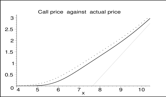
Figure 2: plot of the call price $v$ in terms of $x$ corresponding to an annual interest rate $r=4.5\%$, annual volatility $\sigma=30\%$ and $T-t=1$year with a barrier at $c=4$. Strike is taken as $k=8$. The thick line represents (32) while the dotted line is the BSM call price. Deterministic price is the thin line

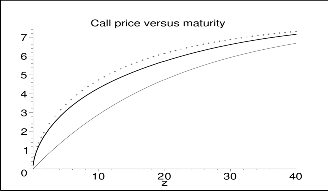
Figure 3: plot of an ATM call option price $v$ in terms of time to maturity $z=T-t$. The thick solid lines represents (32) while the dotted line is the BSM call price. Deterministic price is the thin line. Parameters are as in the previous caption.

4 Appendix

Consider again eq. (4) $dX_{t}=\mu X_{t}dt+b(t,X_{t})dW_{t}$ where $W_{t}$ is a BM with respect to the real world probability and $b(t,x)=\sqrt{2r_{t}\big{(}X_{t}^{2}-c^{2}\big{)}}$. Let

$$u(t,x)\equiv\Big{(}r(t)-\mu\Big{)}x/b(t,x),~{}M_{t}=\exp\Big{(}-\int_{0}^{t}u(s,X_{s})dW_{s}-{1\over 2}\int_{0}^{t}u^{2}(s,X_{s})ds\Big{)}$$

Here $u(t,x)$ is the so called market price of risk . Then if $X_{t}$ solves the above equation $M_{t}$ can be proven formally to be a martingale. Note however that a rigorous proof of the latter fact runs into technical difficulties due to the singularity of $u$ at $x=c$ which might prevent, in principle, for $M_{t}$ to be a Martingale. We skip a rigorous analysis as we expect this to be the case. Defining the risk neutral probability $\mathbb{P}^{*}$ by $d\mathbb{P}^{*}=M_{T}d\mathbb{P}$ it follows from Girsanov’s theorem (see [17,20]) that $W_{t}^{*}\equiv W_{t}+\int_{0}^{t}u(s,X_{s})ds$ is a BM under $\mathbb{P}^{*}$. In this case an easy calculation shows that $X_{t}$ also satisfies Eq. (8) driven by $W_{t}^{*}$, a BM with respect to $\mathbb{P}^{*}$.

5 Bibliography

[1]F. Black, M. Scholes, J. Pol. Econ. 81 (1973) 637-659.

[2] R.C. Merton, Bell J. Econ. Manage. Sci. 4 (1973) 141-183.

[3] M.G. Kendall, J. R. Stat. Soc. 96 (1953) 11-25.

[4] M.F.M. Osborne, Oper. Res. 7 (1959) 145-173.

[5]R. N. Mantegna $\&$ H. E. Stanley, Nature 376, (1995), 46

[6] B. Mandelbrot, J. Bus. 35 (1963) 394

[7]S. Galluzio, G. Caldarelli, M. Marsilli $\&$ Y-C Zhang, Physica A, 245, (1997), 423

[8] A. Matacz, Int. J. Theor. Appl. Finance 3 (2000) 143-160.

[9] J. Masoliver, M. Montero, J.M. Porra, Physica A 283 (2000) 559-567.

[10] J. Masoliver, M. Montero, A. McKane, Phys. Rev. E 64 (2001) 011110

[11]S. Galluzio, Europ. Phys. Jour. B, 20(4),(2001), 595

[12]J. Perelló $\&$ J. Masoliver, Physica A 314, (2002), 736

[13]]J. Perelló $\&$ J. Masoliver, Physica A 308, (2002), 420

[14]J.E. Ingersoll Theory of financial decision making” Rowman $\&$ Littlefield, Savage MD (1987)

[15]J. Hull, ”Options, futures, derivatives”, Prentice Hall Univ.Press, (1997).

[16] D. Duffie, Dynamic Asset Pricing Theory”, Princeton University Press, Princeton (1996)

[17] T. Mikosch, Elementary Stochastic Calculus: with Finance in View, World Scientific, 1998.

[18] J. Voit, ”The statistical mechanics of financial markets”, Springer Verlag, Berlin, (2003)

[19]J.Bouchard $\&$ P.Potters, ”Theory of financial risk, from statistical physics to risk management”, Cambridge Univ. Press, Cambridge 2000

[20] G. Vasconzelos, Braz. Jour. Physics 34(3B), (2004), 1039

[21]R. N. Mantegna $\&$ H. E. Stanley, ”An introduction to Econophysics”, Cambridge Univ. Press, Cambridge (2000)

[22] J.M. Harrison $\&$ S. Pliska, Stochastic Process. Appl. 11 (1981) 215

[23] J.C. Cox, J.E. Ingersoll $\&$ S.A. Ross. Econometrica 53 (2), (1985) 385.

[24] W. Horstheeke and R. Lefever, ”Noise induced transitions, Springer series in synergetics 15, Springer Verlag, Berlin