Precision preparation of strings of trapped neutral atoms

Abstract

We have recently demonstrated the creation of regular strings of neutral caesium atoms in a standing wave optical dipole trap using optical tweezers [Y. Miroshnychenko et al., Nature, in press (2006)]. The rearrangement is realized atom-by-atom, extracting an atom and re-inserting it at the desired position with sub-micrometer resolution. We describe our experimental setup and present detailed measurements as well as simple analytical models for the resolution of the extraction process, for the precision of the insertion, and for heating processes. We compare two different methods of insertion, one of which permits the placement of two atoms into one optical micropotential. The theoretical models largely explain our experimental results and allow us to identify the main limiting factors for the precision and efficiency of the manipulations. Strategies for future improvements are discussed.

1 Introduction

Neutral atoms stored in light induced potentials form a versatile tool for studying quantum many body systems with controlled interactions. One of the most interesting cases occurs if the coherence of such processes is preserved, and hence the build-up of many body quantum correlations can be studied in detail. Such experimental systems are of great interest for quantum information processing [1], and, more general, quantum simulation [2]. Using far detuned optical dipole traps, neutral atoms can be well confined in various geometrical configurations, while at the same time offering long coherence times of their internal states [3, 4].

Two general approaches towards the realization of suitable neutral atom systems can be distinguished: In the typical ”top-down” approach one starts with a large sample of Bose-condensed atoms which are then adiabatically transferred into a three-dimensional optical lattice. A close to perfect array of 10⁵ to 10⁶ atoms is then obtained with almost exactly one atom per site by inducing the Mott insulator state [5]. For this system, the method of spin dependent transport [6] has made possible the creation of large-scale entanglement by inducing controlled, i.e. phase coherent, collisions between neighbouring atoms. However, due to the small distance between adjacent atoms, the manipulation and state detection of individual atoms is still a big challenge.

This problem is overcome in our ”bottom-up” approach where strings of trapped neutral atoms are created one by one. We have experimentally demonstrated [7] that regular strings consisting of up to 7 atoms spaced several potential well apart can be created in a one-dimensional optical lattice. Due to the larger interatomic distance, we are able to address individual atoms reliably [8]. Moreover, the exact number of empty potential wells between two atoms has been measured [9], enabling the method of spin dependent transport in this system.

Small strings of neutral atoms are not only excellent experimental objects to implement controlled coherent collisions, they are also well suited for deterministic coupling using cavity-QED concepts [10]. Here, atom-atom entanglement can be created by synchronous interaction of two atoms with a single mode of the cavity field. Typical modes have diameters of a few 10 $\mu$m, compatible with the interatomic separations on the order of 5-15 $\mu$m in our strings.

In this manuscript we give a detailed analysis of the properties and limitations of our atom sorting apparatus which we use to create such regular strings.

2 Experimental tools

2.1 Standing wave optical dipole traps

We trap neutral caesium atoms in a red-detuned optical standing wave dipole trap, oriented horizontally (HDT) (see figure 1). It is formed by two counter-propagating laser beams with parallel linear polarization, generating a chain of potential well located at the intensity maxima. For a Nd:YAG laser, the periodicity is $\lambda_{\mathrm{HDT}}/2=532$ nm. The beams are focused to a waist radius of $w_{\mathrm{HDT}}=19~{}\mathrm{\mu m}$ yielding a Rayleigh range of 1 mm. An optical power of 1 W per beam results in a measured trap depth of $U_{\mathrm{HDT}}^{0}=0.8$ mK.

Individual atoms trapped in the HDT can be extracted and reinserted with another optical standing wave trap used as optical tweezers. This trap (VDT) is oriented vertically and perpendicularly to the HDT. The standing wave is created by retro reflecting the linearly polarized beam of an Yb:YAG laser ($\lambda_{\mathrm{VDT}}=1030$ nm). This laser beam is focused to a waist radius of $w_{\mathrm{VDT}}=10~{}\mathrm{\mu m}$. The typical power of $0.3$ W creates a measured trap depth of $U_{\mathrm{VDT}}^{0}=1.4$ mK. The power of the VDT laser beam is controlled by an electro optical modulator (EOM).

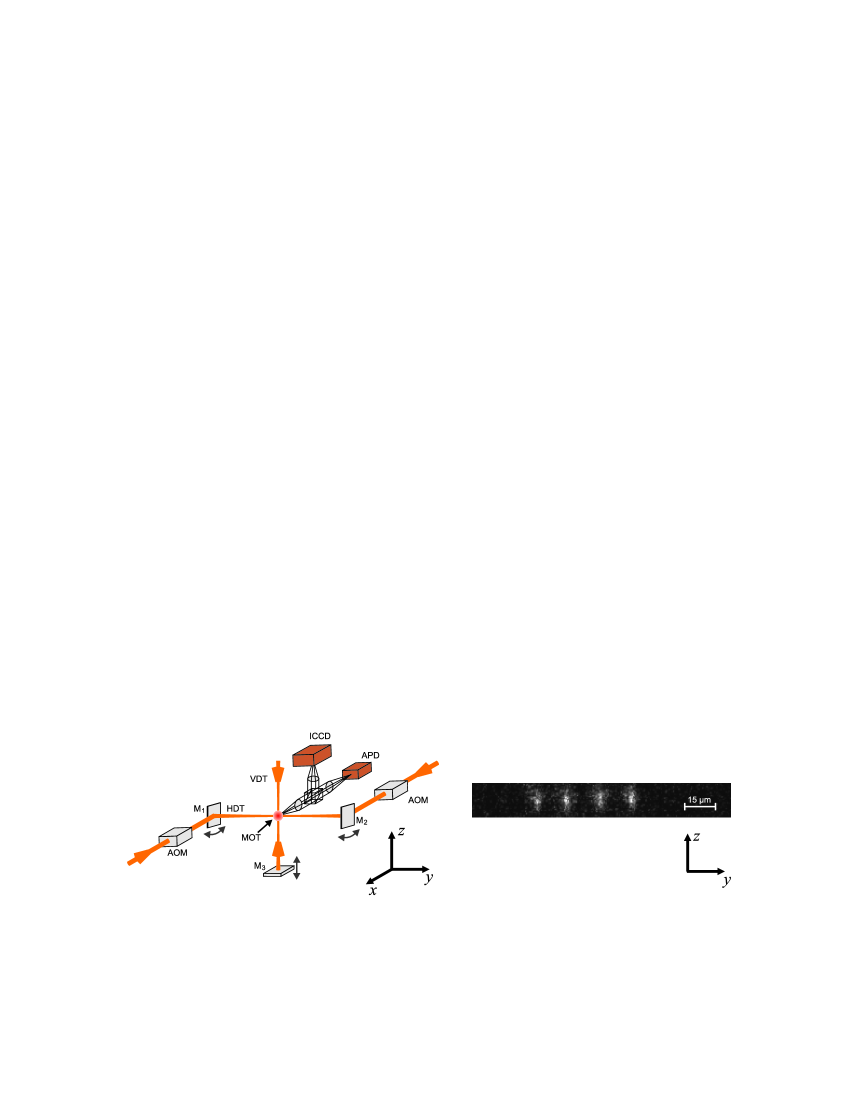
Figure 1: Scheme of the experimental setup for the rearrangement of trapped atoms. Two counter-propagating laser beams produce a horizontally oriented optical standing wave dipole trap (HDT). After loading an exact number of caesium atoms from a magneto-optical trap (MOT) into the HDT, a fluorescence picture, recorded with an intensified CCD camera (ICCD), reveals the initial positions of the atoms. A second, vertically oriented standing wave dipole trap (VDT) is used as optical tweezers to extract a selected atom out of the HDT and to reinsert it at the desired position into the HDT. The ICCD image shows four atoms which have been rearranged into a regular string in the HDT (exposure time 1 s).

2.2 Magneto-optical trap

Our vacuum chamber consists of a glass cell connected to an ultra-high vacuum main chamber and a caesium reservoir separated from the chamber by a valve. An ion getter pump maintains a background gas pressure below $10^{-10}$ mbar.

We use a high gradient magneto-optical trap (MOT) as a source of single atoms for our experiments [11]. The laser system of the MOT consists of two diode lasers in Littrow configuration, frequency-stabilized by polarization spectroscopies. The cooling laser is stabilized to the $F=4\rightarrow F^{\prime}=3/F^{\prime}=5$ crossover transition and shifted by an acousto optic modulator (AOM) to the red side of the cooling transition $F=4\rightarrow F^{\prime}=5$. The $z$-axis of the MOT coincides with the axis of the VDT, whereas the two other axes of the MOT are in the $x$-$y$-plane at $45^{0}$ to the axis of the HDT. The saturation parameter $s=\frac{I}{I_{0}}\left[1+\left(\frac{2\Delta}{\Gamma}\right)^{2}\right]^{-1}$ of each MOT beam is $s=0.5$ ($I$: intensity of the cooling laser; $I_{0}=1.1~{}\mathrm{mW/cm^{2}}$: saturation intensity of the caesium D2 transition; $\Gamma=2\pi\cdot 5.2$ MHz: linewidth of the excited state 6P${}_{3}/2$; $\Delta=1.5~{}\Gamma$: detuning of the cooling laser). The MOT repumping laser is stabilized to the $F=3\rightarrow F^{\prime}=4$ transition. It is linearly polarized and propagates along the axis of the HDT. We typically use $1~{}\mathrm{\mu W}$ focused to about $0.5$ mm.

The high magnetic field gradient of the MOT ($\partial B/\partial z=340$ G/cm) is produced by water cooled magnetic coils mounted symmetrically with respect to the glass vacuum cell. The magnetic field can be switched within 60 ms (mainly limited by the eddy currents in the metal parts of the coils). Due to the high field gradient, the spontaneous loading rate of Caesium atoms from the thermal background vapor into the MOT is negligibly slow.

In order to load the MOT, we temporarily reduce the magnetic field gradient to $\partial B/\partial z=25$ G/cm for the time $\tau_{\mathrm{load}}$ to increase the capture cross section. Varying the loading time $\tau_{\mathrm{load}}$ from few tens to few hundred milliseconds, we can select a specific average number of loaded atoms ranging from 1 to 50.

The atoms are transferred from the MOT into the HDT by simultaneously operating both traps for several tens of milliseconds.

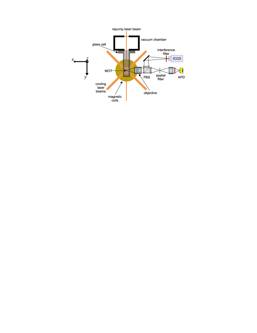
Figure 2: Experimental setup with the detection optics for the MOT fluorescence. The fluorescence light is collected and collimated by an objective. One part of the fluorescence signal is spatially and spectrally filtered and detected with an avalanche photo diode (APD). The other part is only spectrally filtered and sent into an intensified CCD camera.

2.3 Atom detection

The procedures described in this paper rely on our ability to nondestructively determine the exact number and the position of trapped atoms by detecting their fluorescence. For this purpose the fluorescence light is collected by a homemade long working distance microscopic objective (NA=0.29), covering about $2~{}\%$ of the solid angle [12]. The fluorescence is monitored in the time domain by an avalanche photo diode (APD, type SPCM200 CD2027 from EG$\&$G, quantum efficiency $50~{}\%$ at 852 nm) and spatially by an intensified CCD camera (ICCD, type PI-MAX:1K,HQ,RB from Princeton Instruments with image intensifier Gen III HQ from Roper Scientific, quantum efficiency $10~{}\%$ at 852 nm) [13], see figure 2.

2.3.1 Atom number detection

Our atom counting method exploits the fact that each atom contributes equally to the intensity of the MOT fluorescence signal and on the high signal to noise ratio of our detection system, allowing us to distinguish discrete levels in the APD count rate. For $n$ trapped atoms we detect $N_{n}=(R_{\mathrm{stray}}+n\cdot R_{\mathrm{1atom}})\cdot\tau_{\mathrm{int}}$ photons during the integration time $\tau_{\mathrm{int}}$, see figure 3. Here, $R_{\mathrm{stray}}$ is the count rate due to the stray light and the detector background, and $R_{\mathrm{1atom}}$ is the actual one-atom fluorescence rate. For typical MOT parameters we detect $R_{\mathrm{1atom}}=35000/\mathrm{s}$ and $R_{\mathrm{stray}}=25000/\mathrm{s}$.

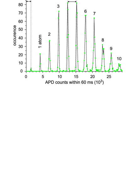
Figure 3: Histogram of the APD counts detected within the integration time $\tau_{\mathrm{int}}=60~{}\mathrm{ms}$ after loading five atoms on average into the MOT (1800 repetitions). The peaks correspond to different number of atoms in the MOT.

The standard deviation of the detected photon number is fundamentally limited by Poisson statistics to $N_{n}^{-1/2}$. Fluctuations of the MOT laser beams including intensity, phase and pointing stability are taken into account in analogy with the description of intensity noise in laser beams by a global relative intensity noise $RIN=\delta N^{2}/N^{2}$ where $\delta N^{2}$ represents the rms-value of these fluctuations. In our case $RIN=0.01^{2}-0.02^{2}$.

In order to distinguish between $n$ and $n+1$ atoms, the total width of the peaks corresponding to neighboring atom numbers ($\Delta N=(N_{n}+RIN\cdot N_{n}^{2})^{1/2}$) has to be compared to their separation $R_{\mathrm{1atom}}\tau_{\mathrm{int}}$. In order to distinguish atom numbers with better than 95% confidence, the ratio

$$k_{n}=\frac{\Delta N}{N_{n+1}-N_{n}}=\left(\frac{R_{\mathrm{stray}}}{R_{\mathrm{1atom}}}+n\right)\sqrt{\frac{1}{(R_{\mathrm{stray}}+nR_{\mathrm{1atom}})\tau_{\mathrm{int}}}+RIN}$$ (1)

must be smaller than $1/4$. In our experiments, RIN begins to dominate this ratio for integration times $\tau_{\mathrm{int}}\simeq 60~{}\mathrm{ms}$. This time was chosen discriminating atom numbers from the APD signal, since it is short compared to other experimental procedures, and longer times do not improve the signal to noise ratio. This method allows us to discriminate 1 to 20 atoms in the MOT with a confidence level above $95~{}\%$.

2.3.2 Atom position detection

The positions of the atoms in the HDT are determined by illuminating them with an optical molasses and detecting the fluorescence with the ICCD camera. At the same time, the optical molasses cools the trapped atoms, enabling continuous observations of up to one minute [13]. We detect about 160 photons per atom on the ICCD camera within the 1 s exposure time. The $y$-positions of the individual atoms trapped in the HDT (see figure 1) are determined by binning the pixels of the ICCD image in the vertical $z$-direction after suitably clipping the image to minimize background noise. The resulting one-dimensional intensity distribution along the $y$-direction is fitted with a sum of Gaussians, which are used as an approximation to the line spread function of our imaging system [9]. We define the centers of the Gaussians as the $y$-positions of the atoms, which can be determined with a precision of 140 nm rms (below the wavelength of the imaging light) within 1500 ms (1000 ms of exposure and 500 ms read-out and image processing). In this way we are able to determine the number of potential wells separating two simultaneously trapped atoms.

Since we want to transport atoms over distances up to 1 mm with submicrometer accuracy, it is essential to obtain a precise calibration of camera pixel to the position in the object plane of the microscope objective.

For this calibration we take advantage of the fact that the atoms in the HDT are trapped in the potential minima separated by exactly $\lambda_{\mathrm{HDT}}/2=532$ nm. Therefore, the measured distance between two simultaneously trapped atoms $d$ given in units of camera pixels must correspond to an integer multiple of $\lambda_{\mathrm{HDT}}/2$ in the object plane:

$$\alpha d=n\lambda_{\mathrm{HDT}}/2,$$ (2)

where $\alpha$ is the calibration parameter in $\mathrm{\mu m/pixel}$. In order to determine $\alpha$ we have first accumulated about 500 images with two to four atoms trapped in the HDT. Then we have determined the interatomic separations in each image, resulting in $n\approx 700$ distance values $d_{i}$, shown in figure 4. In order to avoid any inaccuracy caused by overlapping peaks at short distances, only separations of more than $10~{}\mathrm{\mu m}$ then were taken into account. To find the periodicity of the distribution we construct a function built by summing the delta functions at the positions of each $d_{i}$

$$f(y)=\frac{1}{n}\sum_{i=1}^{n}\delta(d_{i}-y)$$ (3)

and Fourier transform it:

$$g(k)=\frac{1}{\sqrt{2\pi}}\int_{-\infty}^{\infty}f(y)e^{2\pi iky}dy=\frac{1}{\sqrt{2\pi}~{}n}\sum_{i=1}^{n}e^{2\pi ikd_{i}}.$$ (4)

The real part of the Fourier transform of $g(k)$ is shown in figure 4. The most prominent peak at $k_{0}=0.9336(\pm 0.0003)~{}1/\mathrm{pixel}$ corresponds to the spatial frequency of the standing wave pattern:

$$k=\frac{\alpha}{\lambda_{\mathrm{HDT}}/2}~{}~{}.$$ (5)

This yields the calibration parameter $\alpha=0.4967(\pm 0.0002)~{}\mathrm{\mu m/pixel}$.

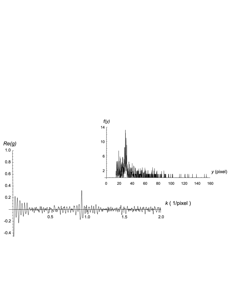
Figure 4: Histogram of measured distances and its fourier transfor. The only one prominent contribution at $k_{0}=0.9336~{}\mathrm{wells/pixel}$ corresponds to the periodicity of $\lambda_{\mathrm{HDT}}/2$ in the object plane of the microscope objective. The inset shows the original function $f(y)$. Here, for presentation purposes each delta function was replaced by a Gaussian with the width of $0.05$ pixel.

The error of this value is dominated by the statistical error due to the finite sample and the $130~{}\mathrm{nm}$-uncertainty in the determination of each distance [9]. The statistical error is estimated by randomly selecting a subset of $n/2$ distances and determining $\alpha$ by the above mentioned calculations on this subset. Using 20 different subsets the standard deviation $(\delta\alpha)_{n/2}$ was determined. The statistical error for the full set is therefore $(\delta\alpha)_{n}=(\delta\alpha)_{n/2}/\sqrt{2}$. The slight modification of the wave length $\lambda_{\mathrm{HDT}}$ in the Rayleigh zone by the Guoy phase is on the order of 10^-5 and hence negligible here.

2.4 Three-dimensional transport of atoms

We transport atoms in the $x$-$y$-plane using the HDT. Vertical transport of the atoms along the $z$-direction is realized by the VDT.

2.4.1 Transportation along the $y$-direction

An “optical conveyor belt” [14] along the trap axis is realized by means of acousto-optic modulators (AOMs) installed in each arm of the HDT, see figure 1. Mutually detuning the AOM driving frequencies using a dual-frequency synthesizer, detunes the frequencies of the two laser beams. As a result, the standing wave pattern moves along the axis of the trap.

The optical conveyor belt allows us to transport the atoms over millimeter distances with submicrometer precision [9, 14] within several milliseconds. The accuracy of the transportation distance is limited to $190~{}\mathrm{nm}$ by the discretisation error of our digital AOM-driver [9]. In this experiment we typically transport atoms over a few tens of micrometers within a few hundred microseconds.

2.4.2 Transportation along the $x$-direction

Displacement of the HDT along the $x$-direction is realized by synchronously tilting the mirrors M₁ and M₂, see figure 1, in opposite directions around the $z$-axis using piezo-electric actuators. For tilt angles below $0.1~{}\mathrm{mrad}$ the variation of the interference pattern is small and to a good approximation pure $x$-translation is realized.

We typically move atoms in the $x$-direction by two times the waist radius of the HDT (ca. $40~{}\mathrm{\mu m}$) with a precision of a few micrometers within 50 ms. The maximum transportation distance is limited to about $40~{}\mathrm{\mu m}$ by the dynamic range of the actuators. The minimal transportation time is limited to about $10~{}\mathrm{ms}$ by the bandwidth of the PZT-system.

2.4.3 Transportation along the $z$-direction

The VDT acts as optical tweezers and extracts and reinserts atoms in the $z$-direction. To axially move the standing wave pattern of the VDT, the retro-reflecting mirror $M_{3}$ is mounted on a linear PZT stage, see figure 1.

In our experiments the VDT transports an atom over about $70~{}\mathrm{\mu m}$ along the $z$-axis by applying a sinusoidal voltage ramp to the PZT within $50~{}\mathrm{ms}$. The precision of the transportation is limited to a few micrometers by the hysteresis of the piezo-crystal, whereas the transportation time is limited by the inertia of the mirror.

3 Positioning individual atoms in the HDT

3.1 Outline of the distance-contlor procedure

Figure 5: Distance-control operation [7]. After the initial positions of all the atoms are determined (a), the rightmost atom is transported to the position of the VDT (b). This atom is extracted vertically with the optical tweezers out of the HDT (c). The rest of the atoms is transported along the axis of the horizontal trap, so that the leftmost atom arrives at the target separation $d_{t}$ from the axis of the VDT (d). The extracted atom is inserted at the desired position into the HDT (e). Note that the fluorescence spots, corresponding to respective atoms, were colored for visualization purposes.

Immediately after loading the HDT with $n\geq 2$ atoms, they are randomly distributed over an interval of about $100~{}\mathrm{\mu m}$ along the axis of the trap. In order to create regular strings with a target interatomic separation $d_{\mathrm{t}}$, atoms are repositioned one by one with the VDT-optical tweezers. For this, the initial positions of all atoms are first determined by recording and analyzing a fluorescence ICCD image, see figure 5(a). Then, the atoms are rearranged in the HDT by sequential application of the “distance-control” operation: The string of atoms in the HDT is transported horizontally along the trap axis, such that the rightmost atom arrives at the $y$-position of the VDT ($y_{\mathrm{VDT}}$), see figure 5(b). After adiabatically switching on the VDT, this atom is transported upwards by approximately three times the waist of the HDT, out of its region of influence.

This atom is then extracted with the optical tweezers (c). The rest of the string in the HDT is transported along the $y$-axis until the leftmost atom of the string arrives at $y_{\mathrm{VDT}}+d_{\mathrm{t}}$ (d). The procedure is completed by reinserting the extracted atom at this position into the HDT (e). Each operation permutes the order of the atoms, and after $n-1$ steps an equidistant string of $n$ atoms is formed. Figure 6 shows ICCD images of equidistant strings of up to seven atoms with interatomic separations of $15~{}\mathrm{\mu m}$.

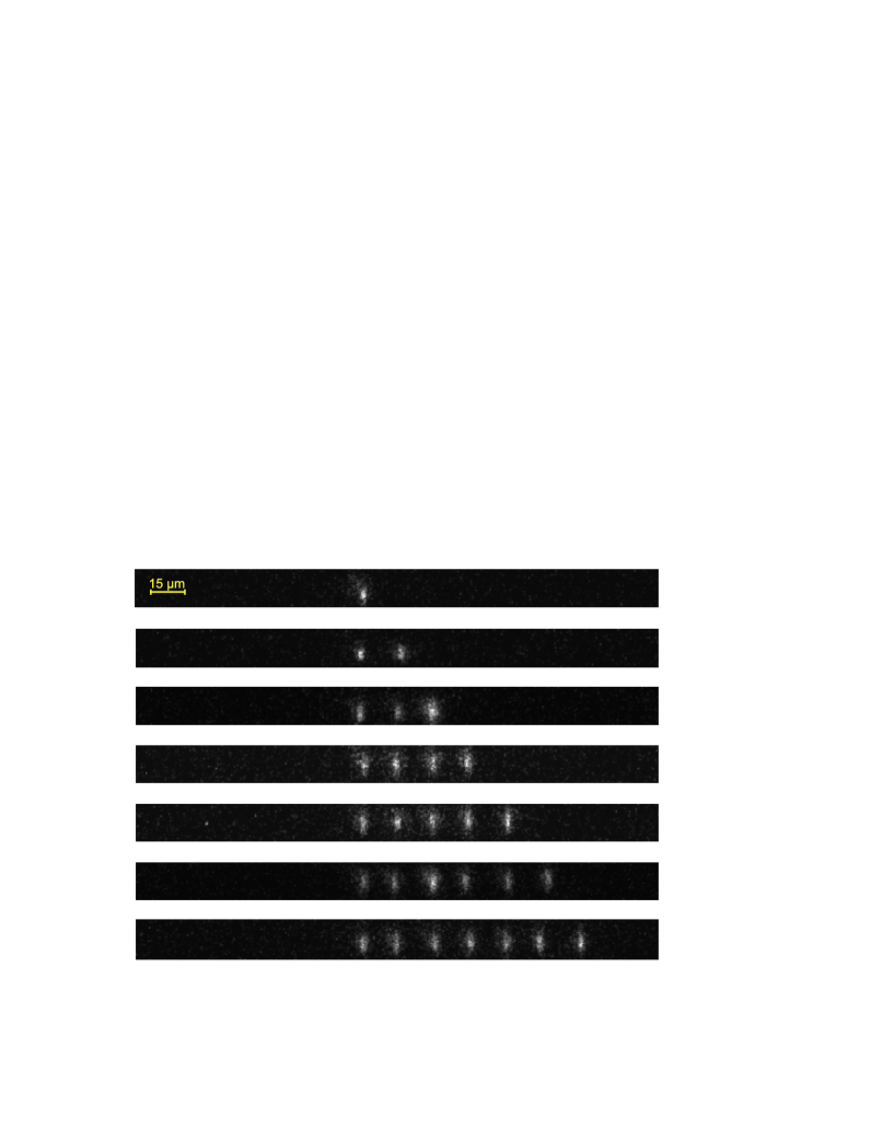
Figure 6: Equidistant strings of $n$ atoms created by rearranging the atoms of the string applying $n-1$ times the distance-control operation.

A perfect distance-control procedure would extract and re-insert an atom with $100~{}\%$ efficiency at a separation to the next atom given in terms of an exactly known number of micropotentials always, i. e., multiple of $\lambda_{\mathrm{HDT}}/2$. We have developed a model of extraction and re-insertion in order to study the physical limitations of the repositioning procedure.

3.2 Extraction of an atom

For extraction, the VDT-optical tweezers needs to overcome the HDT trapping forces. In both the HDT and VDT standing wave dipole traps confinement in the axial direction is almost two orders of magnitude tighter than in the radial direction, the maximal axial forces are thus much larger than the radial forces. For comparable potential depths of the HDT and the VDT, an atom in the overlap region will therefore always follow the axial shift of the traps.

Successful extraction of a single atom not only requires efficient handling of the atoms between the HDT and VDT traps. In addition, other atoms present in the vicinity must remain undisturbed. We have thus defined and analyzed a minimal separation of atoms tolerable on extraction, which is equivalent to an effective “width of the optical tweezers”.

3.2.1 Theoretical model of the width of the optical tweezers

In this model motion in the traps is treated classically, for at the atomic temperature of about $60~{}\mathrm{\mu K}$ for the typical depths of the traps in our experiments the mean oscillatory quantum numbers are $n_{\mathrm{rad}}\approx 90$, $n_{\mathrm{ax}}\approx 3$ for the VDT, and $n_{\mathrm{rad}}\approx 400$, $n_{\mathrm{ax}}\approx 6$ for the HDT.

We consider two crossed standing wave optical dipole traps. For simplicity, we assume that all the spatial manipulations are carried out within the Rayleigh-range of the standing wave dipole traps, i. e., we neglect the change of the curvature of the wave fronts. In this approximation, each dipole trap is described by three parameters: the waist radius of the Gaussian beam, the depth of the trap, and the periodicity of the standing wave. Atoms are trapped in the different potential wells of the standing wave of the HDT and are extracted purely along the $z$-direction. The motion occurs in the $y$-$z$-plane only. Therefore, we consider one-dimensional potentials along the $z$-axis at different $y$-positions in the $y$-$z$-plane with $x=0$.

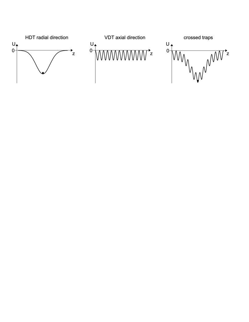
Figure 7: Trapping potentials along the $z$-axis. The trapping potential in the overlap region of the two traps is the sum of the Gaussian profile of the radial confining potential of the HDT and of the standing wave of the VDT. An atom at the bottom of the HDT experiences light forces of the standing wave, too.

In order to separate the effects of the potential shape and the atomic motion on the process of extraction, we first model the case of atoms at zero temperature, where the energy of the atoms is well defined. Later, the influence of the thermal energy distribution is discussed.

Tweezers potential Consider an atom at rest trapped at the bottom of a micropotential of the HDT at $y=0$, which coincides with the axis of the VDT. At this position the HDT-potential in the $z$-direction has a Gaussian shape with waist $w_{\mathrm{HDT}}$ and depth $U_{\mathrm{HDT}}^{0}$. After switching on the VDT, in addition to the Gaussian potential of the HDT, a periodic potential with depth $U_{\mathrm{VDT}}^{0}$ and period $\lambda_{\mathrm{VDT}}/2$ is superimposed in the $z$-direction, see figure 7. Since the HDT and VDT laser frequencies are far apart, the trapping potentials are added incoherently, and the atom is then additionally subject to the forces of the VDT standing wave.

During extraction of the atom during the $z$-direction it is conveyed at the bottom of the micropotential away from the axis of the HDT. Due to the Gaussian radial profile of the HDT, the depth of the local potential minima changes along the $z$-axis and reaches its minimum at the distance $z_{\mathrm{max}}=w_{\mathrm{HDT}}/2$ from the axis of the HDT. Here the slope of the Gaussian is maximal and the effective depth of the local micropotential, see figure 8, can be approximated as

$$U_{\mathrm{eff}}\approx U_{\mathrm{VDT}}^{0}-\frac{1}{\pi\sqrt{e}}\frac{\lambda_{\mathrm{VDT}}}{w_{\mathrm{HDT}}}U_{\mathrm{HDT}}^{0}.$$ (6)

The condition for extracting the atom from the HDT is given by

$$U_{\mathrm{eff}}>0.$$ (7)

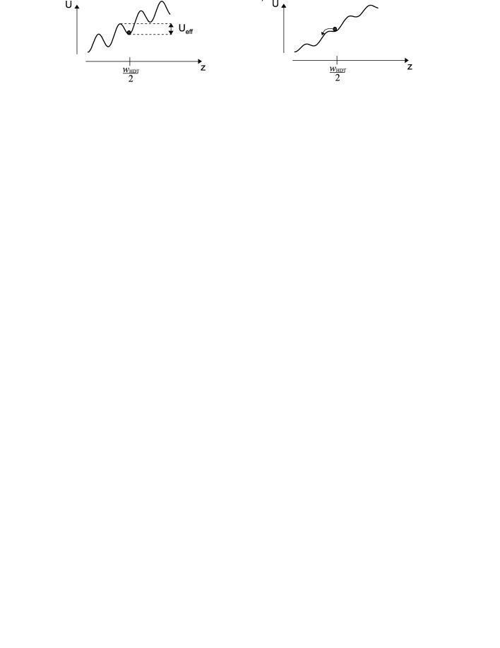
Figure 8: Decrease of the effective depth of the potential well. Due to the Gaussian shape of the confining potential of the HDT in the $z$-direction, the depth of the standing wave pattern reaches its minimum at the distance $w_{\mathrm{HDT}}/2$ from the axis of the HDT. If the effective depth $U_{\mathrm{eff}}$ is greater than zero, the atom remains trapped in the standing wave and will be finally extracted with the VDT a). Otherwise, the atom always rolls down during the extraction b).

Now, consider an atom is trapped at some other position $y\neq 0$ along the HDT. The potential along the $z$-direction will be the sum of the same Gaussian potential well of the HDT with depth $U^{0}_{\mathrm{HDT}}$ and of the periodic potential of the VDT, but now with the reduced depth $U_{\mathrm{VDT}}^{0}~{}e^{-\frac{2y^{2}}{w_{\mathrm{VDT}}^{2}}}$. The sum of the two potentials at the lateral position $y$ generalizes (6) to

$$U_{\mathrm{eff}}(y)\approx U_{\mathrm{VDT}}^{0}~{}e^{-\frac{2y^{2}}{w_{\mathrm{VDT}}^{2}}}-\frac{1}{\pi\sqrt{e}}\frac{\lambda_{\mathrm{VDT}}}{w_{\mathrm{HDT}}}U_{\mathrm{HDT}}^{0}.$$ (8)

Consequently, there exists some region $-y_{\mathrm{T}}<y<y_{\mathrm{T}}$ along the HDT, where condition (7) holds, and where atoms will be extracted by the VDT. Figure 9(a) shows the probability $p_{\mathrm{noextr}}$ for an atom to remain trapped in the HDT after the extraction as the function of the lateral position $y$. The critical position $y_{\mathrm{T}}$ defined by the condition $U_{\mathrm{eff}}(y_{\mathrm{T}})=0$ is

$$y_{\mathrm{T}}=\frac{w_{\mathrm{VDT}}}{\sqrt{2}}\sqrt{\ln\left(\pi\sqrt{e}\frac{w_{\mathrm{HDT}}}{\lambda_{\mathrm{VDT}}}\frac{U_{\mathrm{VDT}}^{0}}{U_{\mathrm{HDT}}^{0}}\right)}~{}~{}.$$ (9)

Figure 9: Probability for an atom not to be extracted from the HDT. a) atoms at $T=0~{}\mathrm{K}$. b) atoms at temperatures $T_{1}$ (solid line) and $T_{2}$ (dashed line), with $T_{1}>T_{2}$.

This equation characterizes the width of the optical tweezers, $y_{\mathrm{T}}$, as a function of the trap parameters for atoms at zero temperature. It shows that the lowering of $U_{\mathrm{VDT}}^{0}$ reduces the extraction width $2y_{\mathrm{T}}$, from which the atoms will be extracted. For $T=0~{}\mathrm{K}$ and neglecting quantum effects, this region can be made arbitrary small at $U_{\mathrm{VDT}}^{0}=\frac{\lambda_{\mathrm{VDT}}}{\pi\sqrt{e}w_{\mathrm{HDT}}}U_{\mathrm{HDT}}^{0}$.

Thermal atomic motion We now model atomic motion in the dipole trap by an ensemble in thermal equilibrium at temperature $T$ in a three-dimensional harmonic potential. We assume that the energy of the atoms is Boltzmann-distributed [15]:

$$f(E,T)=\frac{1}{2(k_{\mathrm{B}}T)^{3}}E^{2}e^{-E/(k_{\mathrm{B}}T)}.$$ (10)

For an atom with a fixed energy $E$ the condition for the extraction analogous to (7) is

$$U_{\mathrm{eff}}(y)-E>0~{}.$$ (11)

For a given temperature $T$ the fraction of atoms with an energy above $U_{\mathrm{eff}}$ is given by

$$p(U)=\int_{\max{\{U_{\mathrm{eff}},0\}}}^{\infty}f(E,T)dE~{},$$ (12)

which therefore is the fraction $p_{\mathrm{noextr}}$ of the atoms not extracted from the HDT. As a function of the lateral position $y$ we have

$$p_{\mathrm{noextr}}(y)\equiv p(U_{\mathrm{eff}}(y))=\frac{1}{2}\left[\left(~{}\frac{U_{\mathrm{eff}}(y)}{k_{\mathrm{B}}T}+1\right)^{2}+1\right]\exp\left({-\frac{U_{\mathrm{eff}}(y)}{k_{\mathrm{B}}T}}\right).$$ (13)

Figure 9(b) shows $p_{\mathrm{noextr}}$ for the same trap parameters as in figure 9(a). Atomic motion causes “softening” of the edges of the extraction zone. An increasing temperature causes narrowing of the region of efficient extraction.

Here we define the region influenced by the optical tweezers $[-y_{\mathrm{T}},y_{\mathrm{T}}]$, see figure 9(b), by

$$p_{\mathrm{noextr}}(y_{\mathrm{T}})\leq 0.99.$$ (14)

In order to optimize the extraction resolution we vary $U_{\mathrm{VDT}}^{0}$ such that $y_{\mathrm{T}}$ is minimal while still guarantying efficient extraction in the center. We therefore choose $U_{\mathrm{VDT}}^{0}$ fulfilling the condition

$$p_{\mathrm{noextr}}(y=0)=0.01$$ (15)

and get the minimal region of influence $[-y_{\mathrm{T}}^{\mathrm{opt}},y_{\mathrm{T}}^{\mathrm{opt}}]$ from

$$p_{\mathrm{noextr}}(y_{\mathrm{T}}^{\mathrm{opt}})=0.99.$$ (16)

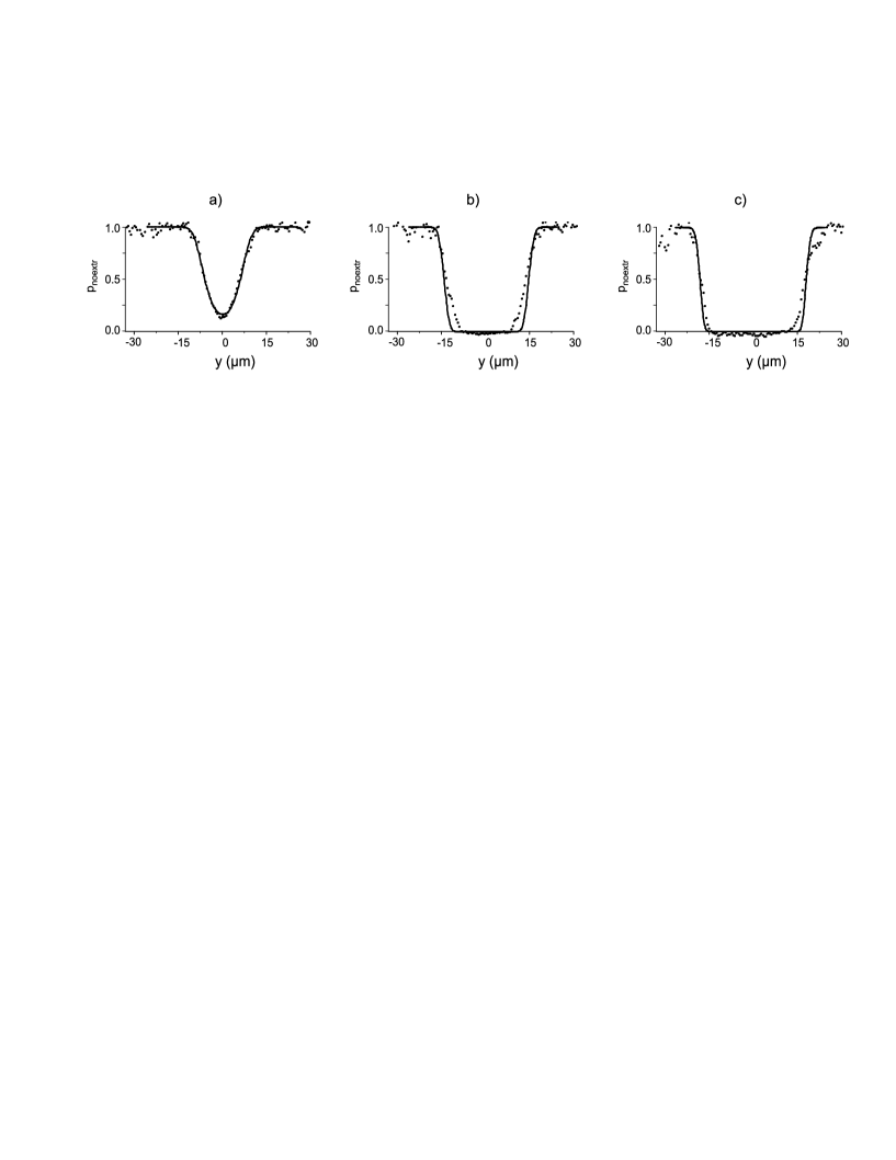
Figure 10: Comparison of the experimental data and the respective theoretical expectation. a) Fit of $P_{\mathrm{HDT}}$ (solid line) to the experimental data (points) for $U^{0}_{\mathrm{VDT}}/k_{\mathrm{B}}=0.3$ mK. b,c) The function $P_{\mathrm{HDT}}$ with parameters from a) except $U_{\mathrm{VDT}}^{0}/k_{\mathrm{B}}=3.1$ mK and $U_{\mathrm{VDT}}^{0}/k_{\mathrm{B}}=16.8$ mK, respectively. The depth of the HDT is $U_{\mathrm{HDT}}^{0}/k_{\mathrm{B}}=0.8$ mK.

3.2.2 Measurement of the width of the optical tweezers

We have experimentally determined the width $2y_{\mathrm{T}}$ of the optical tweezers as a function of the depth of the VDT by loading the HDT with atoms distributed over a region larger than $y_{\mathrm{T}}$, extracting atoms with the VDT, and analyzing the distribution of the atoms remaining in the HDT. Images of the atoms in the HDT were taken before and after extraction, and used to calculate the probability $P_{\mathrm{HDT}}(y)$ of the atoms to remain trapped in the HDT after the extraction. In this measurement, the depth of the HDT was fixed ($U_{\mathrm{HDT}}^{0}/k_{\mathrm{B}}=0.8$ mK), whereas the depth of the VDT was varied over two orders of magnitude from 0.3 to 16.8 mK. The corresponding plots for $U^{0}_{\mathrm{VDT}}/k_{\mathrm{B}}=0.3$ mK, $3.1$ mK and $16.8$ mK are presented in figure 10.

3.2.3 Analysis

In figure 10, the measured data are compared to the theoretical model described by (13). Free fit parameters for the data of figure 10(a) include the temperature $T$ of the atoms, the waist of the VDT $w_{\mathrm{VDT}}$ along the axis of the HDT, and the position of the VDT $y_{0}$, relative to the picture. The fit to the data set for the depth of the VDT at $U^{0}_{\mathrm{VDT}}/k_{B}=0.3$ mK, corresponding to a power of the incoming VDT laser beam of 0.06 W, yields

$$T=60(\pm 1)~{}\mathrm{\mu K}~{}~{}~{}\mathrm{and}~{}~{}~{}w_{\mathrm{VDT}}=11.6(\pm 0.2)~{}\mathrm{\mu m},$$

see figure 10(a). The temperature thus obtained is in the range of the typical temperatures measured by other methods [16]. Whereas the error is probably too small and underestimate the systematic influence of the approximations of the model. Also, the fitted value of the waist of the VDT is in reasonable agreement with the value of $10.1(\pm 1.4)~{}\mathrm{\mu m}$ determined from the oscillation frequency measurements. In figure 10(b) and (c) we have plotted the model function $p_{\mathrm{noextr}}(y)$ at $U_{\mathrm{VDT}}^{0}/k_{\mathrm{B}}=3.1$ mK and $U_{\mathrm{VDT}}^{0}/k_{\mathrm{B}}=16.8$ mK, respectively, without further adjustment of $T$ and $w_{\mathrm{VDT}}$, finding good agreement with the experimental data.

Using the quantitative definitions (15) and (16) we can determine the optimal width of the optical tweezers for our current experimental parameters, i. e., for the depth of the HDT of $0.8$ mK and the atomic temperature of $T=60~{}\mathrm{\mu K}$. Using (15) we find the optimal depth of the VDT at $U_{\mathrm{VDT}}^{0}/k_{\mathrm{B}}=0.5$ mK. The corresponding width of the optical tweezers is calculated with (16) to be $2y_{\mathrm{T}}^{\mathrm{opt}}=2\cdot 11.7~{}\mathrm{\mu m}$, see Tab. 1.

Table 1: Width of the tweezers $2y_{\mathrm{T}}^{\mathrm{opt}}$ for different parameters

	$\frac{U_{\mathrm{HDT}}^{0}}{k_{\mathrm{B}}}~{}$(mK)	$\frac{U_{\mathrm{VDT}}^{0}}{k_{\mathrm{B}}}~{}$(mK)	$T~{}(\mathrm{\mu K})$	$\frac{w_{\mathrm{HDT}}}{\lambda_{\mathrm{VDT}}}$	$\frac{w_{\mathrm{VDT}}}{\lambda_{\mathrm{VDT}}}$	$F_{\mathrm{r}}$	$y_{\mathrm{T}}^{\mathrm{opt}}~{}(\mathrm{\mu m})$
	current experiment
1	0.8	0.51	60.0	19	9.8	0.015	11.7
	stronger focusing of optical tweezers
2	0.8	0.51	60.0	19	4.9	0.025	5.9
3	0.8	0.51	60.0	19	2.45	0.025	2.9
	lower atom temperature
4	0.8	0.017	1.0	19	4.9	0.482	2.9
5	0.8	0.0088	0.084	19	2.45	0.920	0.5

3.2.4 Towards ultimate resolution

Ultimate resolution of the optical tweezers is realized, if a single potential well of the HDT is addressed only. Here, we use our model in order to develop strategies for the reduction of the width of our optical tweezers. It depends on the depth and waist of the VDT, of the HDT, and on the temperature of the atoms. Experimentally, variation of the depth of the traps is straight forwardly realized by changing the power of the respective laser (up to 20 W for the VDT laser and 1.2 W for each beam for the HDT laser). Changing the waist size of the traps requires a new lens system, and lowering of the atomic temperature could be achieved by e. g. Raman sideband cooling technique [17].

In the following analysis we ignore further experimental effects not included in our model, e. g., drifts of the traps, fluctuations of the trap depths, or heating in the traps, which become relevant for ultimate precision.

Universal extraction function In order to introduce dimensionless parameters, we rewrite (8) in the form

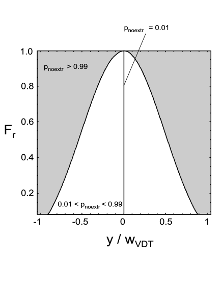
Figure 11: Contour plot for $p_{\mathrm{noextr}}(y_{\mathrm{T}}^{\mathrm{opt}},F_{\mathrm{r}})=0.99$. Outside the white area atoms will remain trapped in the HDT with 99 % probability.

$$\frac{U_{\mathrm{eff}}(y)}{k_{\mathrm{B}}T}=s_{\mathrm{T}}\left(e^{-\frac{2y^{2}}{w_{\mathrm{VDT}}^{2}}}-F_{\mathrm{r}}\right),$$ (17)

where the normalized tweezers potential depth is

$$s_{\mathrm{T}}=\frac{U_{\mathrm{VDT}}^{0}}{k_{\mathrm{B}}T}$$ (18)

and

$$F_{\mathrm{r}}=\frac{1}{\pi\sqrt{e}}~{}\frac{U_{\mathrm{HDT}}^{0}}{U_{\mathrm{VDT}}^{0}}~{}\frac{\lambda_{\mathrm{VDT}}}{w_{\mathrm{HDT}}}$$ (19)

is a relative measure of the forces exerted by the HDT ($\sim U_{\mathrm{HDT}}^{0}/w_{\mathrm{HDT}}$) compared to VDT ($\sim U_{\mathrm{VDT}}^{0}/\lambda_{\mathrm{VDT}}$). The condition of the extraction (7) translates into

$$F_{\mathrm{r}}<1.$$

The condition (15) that the target atom is efficiently extracted out of the HDT, is satisfied for

$$s_{\mathrm{T}}=\frac{8.4}{1-F_{\mathrm{r}}}.$$ (20)

Now we rewrite (16) in terms of the dimensionless parameters $s_{\mathrm{T}}$ and $F_{\mathrm{r}}$ and use the substitution 20 to find the connection between the optimal width of the optical tweezers $y_{\mathrm{T}}^{\mathrm{opt}}$ and the dimensionless parameter $F_{\mathrm{r}}$:

$$p_{\mathrm{noextr}}(y_{\mathrm{T}}^{\mathrm{opt}},F_{\mathrm{r}})=0.99,$$ (21)

which is plotted in figure 11.

From this figure we can already infer two strategies for improved resolution: the value of $F_{\mathrm{r}}$ should be about unity, and the waist of the VDT should be as small as possible. $F_{\mathrm{r}}$ can be increased by increasing the depth of the HDT, by reducing $w_{\mathrm{HDT}}$ and by lowering the temperature $T$ of the atoms, see (19) and (18).

Examples of optical tweezers In Table 1 we have listed possible parameters for the traps which would improve the extraction resolution. In line 1 we have optimized $U_{\mathrm{VDT}}^{0}$ for our experimental parameters. In lines 2-3 we project parameters for improved resolution by changing the focus of the VDT, in lines 4 and 5 the effect of lower temperatures is shown (about 1 $\mu$K and 0.1 $\mu$K which can be obtained with Raman cooling [18] and quantum degenerate gases).

3.3 Insertion of an atom

After extraction, the atom is trapped in the potential of the VDT. In order to re-insert the atom into a potential well of the HDT, the VDT potential is merged with the HDT and finally switched off. There are two alternative methods to insert an atom back into the HDT: “axial insertion” and “radial insertion”.

Axial insertion In this case, the process of extraction of an atom is simply reversed: the VDT axially transports the atom to the axis of the HDT, see figure 12, and then the VDT is adiabatically switched off, leaving the atom in the HDT. The whole process of axial insertion takes about $70~{}\mathrm{ms}$.

Radial insertion For radial insertion, the two traps are first radially separated by displacing the axis of the HDT in the positive $x$-direction, see figure 13(a). Then the atom in the VDT is transported downwards to the vertical position of the horizontal trap, see figure 13(b).

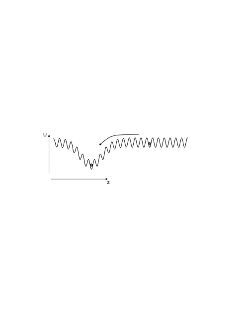
Figure 12: Axial insertion. An atom trapped in one of the potential wells of the standing wave of the VDT, is inserted into the Gaussian potential well of the HDT by axially moving the VDT along the $z$-direction.

Along the $x$-axis, the atom in this configuration is confined in the Gaussian-shaped radial potential of the VDT. In the next step, the VDT is then merged with the Gaussian-shaped radial potential of the HDT by moving the HDT radially towards the $x$-position of the VDT, see figure 13(c). In the final step the VDT is adiabatically switched off, which releases the atom to the HDT, see figure 13(d). The process of radial re-insertion takes about $210~{}\mathrm{ms}$.

A radical difference of the two alternative insertion methods occurs if the HDT already holds an atom within the width of the optical tweezers. During axial insertion the VDT exerts the same forces as during the extraction of an atom. Therefore, the achievable final distance between two atoms in the HDT is limited to the width of the optical tweezers, because atoms within the extraction region will be extracted downwards by the VDT during the re-insertion. In contrast, if the two traps are merged radially, the VDT does not exert any forces which could push an atom out of the HDT. Consequently, for radial insertion there are no limitations on the final separations. In particular, the final distance between two atoms could be set to zero. In this way, two atoms could be joined in a single micropotential of the standing wave of the HDT. A disadvantage of the radial insertion is additional heating of the atom in the HDT, see Sec. 3.3.

The ultimate goal of insertion is to reliably place an atom into a given micropotential of the HDT, for instance an integer number of potential wells away from the neighboring atom, but without influencing it.

3.3.1 Insertion precision

There are two independent effects influencing the precision of the insertion, i. e., how accurately an atom can be placed at a desired position of the HDT: the thermal motion in the VDT and the position fluctuations of the VDT relative to the HDT. Both of them equally affect the axial and the radial insertion. Therefore, the following theory applies to both methods of insertion.

Thermal distribution in the VDT Before contact with the HDT atoms in the VDT are distributed thermally along the $y$-direction (the axis of the HDT) in an approximately harmonic potential with oscillation frequency $\Omega_{\mathrm{rad}}=\sqrt{\frac{4U^{0}_{\mathrm{VDT}}}{mw_{\mathrm{VDT}}^{2}}}$. It is known that the distribution in this case is a Gaussian,

$$p_{\mathrm{T}}(y)=\sqrt{\frac{m\Omega_{\mathrm{rad}}^{2}}{2\pi k_{\mathrm{B}}T}}e^{-m\Omega_{\mathrm{rad}}^{2}y^{2}/(2k_{\mathrm{B}}T)}.$$ (22)

The width of this distribution

$$\delta y_{\mathrm{therm}}=\frac{w_{\mathrm{VDT}}}{2}\sqrt{\frac{k_{\mathrm{B}}T}{U_{\mathrm{VDT}}^{0}}}$$ (23)

can also be expressed in terms of the VDT waist radius and the $s_{\mathrm{T}}$-parameter, combining $U_{\mathrm{VDT}}^{0}$ and the temperature, see (18):

$$\delta y_{\mathrm{therm}}=\frac{w_{\mathrm{VDT}}}{2s_{\mathrm{T}}^{1/2}}~{}.\\ \\$$ (24)

Spatial fluctuations of the VDT Since the VDT and the HDT laser beams are guided by independent mechanical setups, their relative position is subject to radial and axial fluctuations. In our model these fluctuations are taken into account by $\delta y_{\mathrm{fluct}}$ representing the rms-amplitude of the fluctuations of the VDT axis.

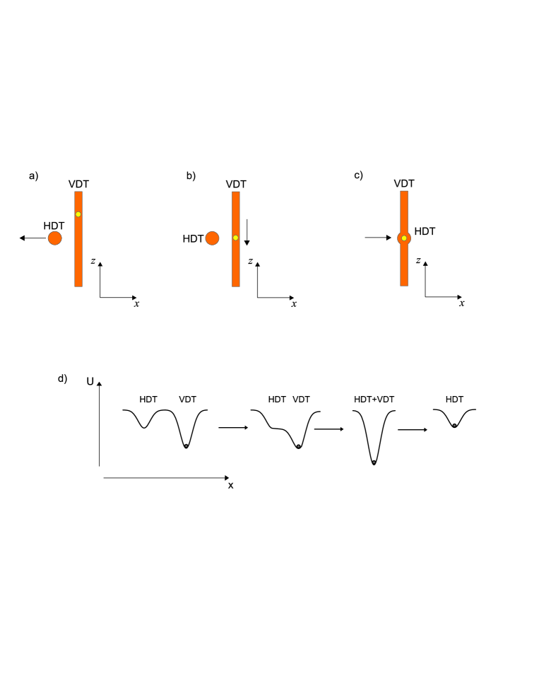
Figure 13: Radial insertion of an atom. a) An atom in the VDT after the extraction. The traps are separated by displacing the HDT along the $x$-direction. b) The atom in the VDT is transported to the $z$-position of the HDT. c) The traps are merged by moving the HDT along the $x$-direction towards the VDT. d) Evolution of the radial potentials of the traps along the $x$-axis for steps b) and c).

For our typical experimental parameters, the width of the thermal distribution is on the order of $0.5~{}\mathrm{\mu m}$, and $\delta y_{\mathrm{fluct}}$ is about $0.5~{}\mathrm{\mu m}$. Assuming these fluctuations are Gaussian distributed the rms-amplitude of the combined fluctuation is:

$$\delta y_{\mathrm{insert}}=\sqrt{\delta y_{\mathrm{therm}}^{2}+\delta y_{\mathrm{fluct}}^{2}}~{}.$$ (25)

The value of $\delta y_{\mathrm{insert}}\approx 0.7~{}\mathrm{\mu m}$ is the width of the distribution of the probability to find an atom along the HDT axis $p(y)$. Since this value is larger than the size of one HDT micropotential, the distribution extends over several potential wells, see figure 14(a).

Insertion into HDT micropotentials by “projection” In the last step of the insertion, the traps are merged and the VDT is finally switched off. Due to the periodicity of the HDT, the distribution $p(y)$ is changed: its envelope reflects the width of the original distribution before the traps were merged, but under this envelope the distribution is now modulated with the periodicity of the standing wave of the HDT, see figure 14(b).

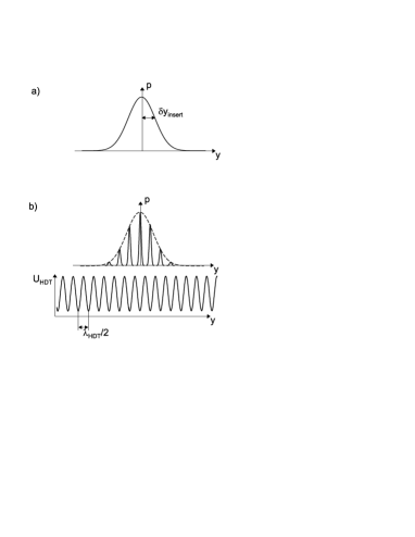
Figure 14: Spatial distribution $p(y)$ with the width $y_{\mathrm{insert}}$ is projected onto the standing wave of the HDT as both traps are merged (a). This distribution after the projection (b). The width of the envelope remains almost unchanged, but the probability is spatially modulated with the periodicity of the HDT.

In harmonic approximation, the distribution in each micropotential is described again by a Gaussian of width

$$\delta y_{\mathrm{micropot}}=\frac{\lambda_{\mathrm{HDT}}}{2\sqrt{2}\pi}\sqrt{\frac{k_{\mathrm{B}}T}{U_{\mathrm{HDT}}^{0}}},$$

where $T$ is the temperature.

It is clear that the insertion precision will be improved by better localization of the atoms, i. e., with lower atomic temperature and deeper VDT potentials. Ultimately, for $\delta y_{\mathrm{insert}}\ll\lambda_{\mathrm{HDT}}/2$ the final distribution will be concentrated into a single micropotential. This limit corresponds to “perfect” insertion.

3.3.2 Experimental studies of the insertion precision

We have carried out a series of measurements in order to experimentally study the dependence of the insertion precision on atomic temperature and on the depth of the VDT predicted by the above model. For this purpose we have loaded atoms into the HDT and extracted the rightmost atom with the VDT, the rest of the atoms was expelled out of the HDT by switching it off for 30 ms. The events with no or too closely spaced atoms were discarded. The atom in the VDT was then cooled with optical molasses, and placed back into the HDT using the method of axial re-insertion. The final positions of the inserted atoms were determined and the standard deviation $\delta y_{\mathrm{insert}}$ was calculated. For $\delta y_{\mathrm{insert}}\gtrsim 0.5\lambda_{\mathrm{HDT}}$ we can neglect the discretization of the positions due to the periodic structure of the HDT [19].

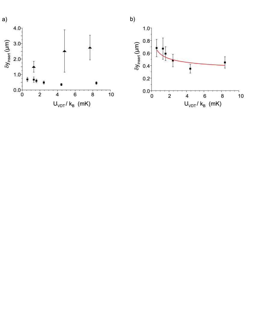
Figure 15: a) Insertion precision as a function of the depth of the VDT. The triangular points present the insertion precision for the experimental sequence without cooling of the atoms before re-insertion. The rectangular points are the results of the insertion precision with the cooling step. b)Zoom of a) showing the data for precooled atoms. The solid line is the fit of (26) to the experimental data. In this experiment we have used the axial insertion method. Every point corresponds to about 25 repetitions of the experiment.

3.3.3 Analysis

Figure 15(a) shows the dependence of the measured insertion accuracy $\delta y_{\mathrm{insert}}$ on the depth of the VDT. The corresponding graph for the radial insertion, see figure 18(b), shows comparable insertion precision as expected.

Temperature of the atoms The temperature was varied by performing the measurement with (squares) and without the cooling step in the VDT (triangles). The huge difference in $\delta y_{\mathrm{insert}}$ qualitatively demonstrates the temperature dependency of the insertion precision and points out the importance of the cooling step. The extraction process itself can heat up the atom if it is initially not located on the VDT axis: the atom remains at its $y$-position until it is released from its HDT potential well and starts to oscillate radially in the VDT. Therefore we have to cool the atom before insertion to achieve a good insertion precision.

Depth of the VDT In order to insert the atoms at different $U_{\mathrm{VDT}}$, we have first extracted and cooled the atoms at a fixed depth $U_{\mathrm{VDT}}^{\mathrm{extr}}$ to insure constant cooling parameters, and then adiabatically changed the depth to $U_{\mathrm{VDT}}$. During this ramp, the temperature of the atoms adiabatically changes to $T=T_{0}\sqrt{U_{\mathrm{VDT}}/U_{\mathrm{VDT}}^{\mathrm{extr}}}$  [16]. Using this temperature in (25) and (23) we obtain the expected insertion precision

$$\delta y_{\mathrm{exp}}(U_{\mathrm{VDT}})=\sqrt{\frac{b^{2}}{\sqrt{U_{\mathrm{VDT}}/k_{\mathrm{B}}}}+\delta y_{\mathrm{fluct}}^{2}}.$$ (26)

The parameter $b=\frac{w_{\mathrm{VDT}}}{2}\frac{\sqrt{T_{0}}}{\sqrt[4]{U_{\mathrm{VDT}}^{\mathrm{extr}}/k_{\mathrm{B}}}}$ is a combination of the waist of the VDT, of the trap depth where the atom was cooled and the temperature. We have independently determined $\delta y_{\mathrm{fluct}}=0.26(\pm 0.03)~{}\mathrm{\mu m}$ by measuring the position of an atom in the VDT over the typical duration of an experimental run (200 sec). Equation (26) was then fitted to the experimental data with the fit parameter $b$, see figure 15(b), yielding $b=0.52(\pm 0.05)~{}\mathrm{\mu m}~{}\mathrm{mK}^{1/4}$.

Using $U_{\mathrm{VDT}}^{\mathrm{extr}}/k_{\mathrm{B}}=1.6(\pm 0.3)~{}\mathrm{mK}$ and the independently measured $w_{\mathrm{VDT}}=10.1(\pm 1.4)~{}\mathrm{\mu m}$ we calculate the corresponding temperature of the atom in the VDT after the cooling step to be $T_{0}=13(\pm 4)~{}\mu K$. This temperature is smaller than the typical temperatures measured in the HDT. The difference between these values could be explained by the fact that the multi mode operation of our HDT laser impairs the cooling process in the HDT [21], or by systematic errors due to approximations in our model.

Periodicity of the HDT Until now we have analyzed the insertion precision in the frame of reference of our ICCD camera. Much more important is the insertion precision relative to a fixed point in the HDT, e. g., another atom. Here we have prepared a pair of atoms with a fixed separation using our distance-control operation, Sec. 3.1. Instead of final positions we now measure final distances, see figure 16. Here the periodicity of the HDT is clearly visible as it is expected from figure 14(b). In the distance measurement the random axial shot–to–shot fluctuations of the HDT standing wave pattern cancel out, whereas in position measurements relative to the ICCD this modulation is smeared out.

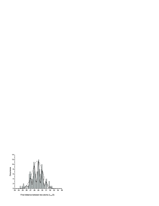
Figure 16: Distribution of the separations between two simultaneously trapped atoms after setting their distance to $15~{}\mathrm{\mu m}$ with our distance-control operation [20]. The histogram clearly shows that the distances are integer multiples of the standing wave period $\lambda_{\mathrm{HDT}}$/2, and extending over only about 4 standing wave potential wells. The solid line is a theoretical fit with a Gaussian envelope (dashed line) centered at $15.31~{}\mu m$ and having a $1/\sqrt{e}$-halfwidth of $0.71~{}\mu m$. The narrow peaks under this envelope have a $1/\sqrt{e}$-halfwidth of $0.130~{}\mu m$, corresponding to the precision of an individual distance measurement [9].

The insertion precision relative to a second atom in the HDT is on the same order of magnitude as $\delta y_{\mathrm{insert}}$ measured in the previous section. This allows us to set a distance between two atoms with an accuracy corresponding to about four potential wells of the HDT.

3.4 Insertion induced heating

As discussed in section 3.3, the method of radial insertion allows us to place an atom arbitrary close to other atoms in the HDT. It turns out that during this insertion an atom in the HDT at the position of the VDT is heated up. This heating effect limits the usable depth of the VDT, such that a compromise between a high precision of insertion and tolerable heating is required.

3.4.1 Adiabatic model

Consider an atom trapped in the HDT at the $y$-position of the VDT, when the traps are axially separated along the $x$-direction. Along this direction the potential is the sum of two Gaussians, i. e., the radial potentials of the two traps. Just before the two traps are merged, the potential shape is shown in figure 17. For $k_{\mathrm{B}}T\ll U_{\mathrm{HDT}}^{0}$, the atom stays near the bottom of the HDT potential until it falls down into the VDT potential. With respect to the bottom of this potential, it has an energy of approximately $E_{\mathrm{a}}\approx U_{\mathrm{VDT}}^{0}-U_{\mathrm{HDT}}^{0}$.

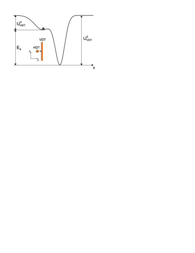
Figure 17: Radial potential of the two traps. During the radial merging of the traps, an atom in the radial potential of the HDT has a potential energy $E_{\mathrm{a}}$ relative to the bottom of the potential well of the VDT. The inset shows the respective geometry of the traps.

Adiabatically switching off of the VDT causes the atom to be adiabatically cooled to the final atomic energy [16]:

$$E_{\mathrm{a}}^{\mathrm{final}}\approx E_{\mathrm{a}}\sqrt{\frac{U_{\mathrm{HDT}}^{0}}{U_{\mathrm{HDT}}^{0}+U_{\mathrm{VDT}}^{0}}},$$ (27)

where the difference between $w_{\mathrm{VDT}}$ and $w_{\mathrm{HDT}}$ has been neglected. The condition for the atom to remain trapped in the HDT is $E_{\mathrm{a}}^{\mathrm{final}}<U_{\mathrm{HDT}}^{0}$, yielding an upper limit for the depth of the VDT

$$U_{\mathrm{VDT}}^{0}\lesssim 3U_{\mathrm{HDT}}^{0},$$ (28)

otherwise the atom will be lost.

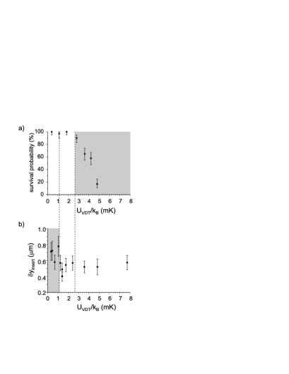
Figure 18: Optimal depth of the VDT. a) The survival probability of an atom in the HDT as a function of the depth of the VDT. Every point is the result of about 35 repetitions of the experiment. b) The insertion precision as a function of the depth of the VDT. Every point corresponds to about 35 radial insertions with a single atom. The shaded areas show the experimentally unfavorable ranges of the depth of the VDT.

3.4.2 Measurement of the heating effect

One atom on average was loaded into the HDT and transported to the $y$-position of the VDT axis. For the third step, the HDT with the atom was transported in the $x$-direction, and the VDT was switched on. At the fourth step, the atom was transported back towards the VDT as it would occur during the radial insertion. Thereafter, the VDT was adiabatically switched off. The final image reveals then the presence or loss of the atom in the HDT. Figure 18(a) shows the survival probability of the atom after this manipulation.

3.4.3 Analysis

The experimental data in figure 18(a), show that starting from a VDT depth of about 2.5 mK, the atoms in the HDT were heated up and lost during the radial insertion procedure. Since the depth of the HDT for this experiment was 0.8 mK, the condition (28) results in $U_{\mathrm{VDT}}^{0}<2.4$ mK, which reasonably agrees with the experimentally observed value.

At the same time, the lower limit on the depth of the VDT is dictated by the insertion precision, which deteriorates with the reduction of the VDT depth. Figure 18(b) shows the insertion precision, measured for the same depth of the HDT using the radial insertion method. For VDT depths below 1.2 mK the insertion precision is dominated by the thermal component and starts to deteriorate, see (23).

The non shaded regions in figure 18 indicate the range of experimentally useful depths of the VDT. For our typical experimental parameters there is a non empty overlap of these regions. It can be further enlarged by increasing the depth of the HDT according to (28).

3.5 Conclusion

Using optical tweezers we have repositioned individual atoms inside a standing wave optical dipole trap with a precision on the order of the periodicity of the trap. Regular string containing 2 to 7 atoms have been prepared atom–by–atom. We have modeled and experimentally analyzed the processes of extraction and insertion of a single atom in detail. We have identified the main limiting factors and proposed strategies for future improvements.

We demonstrate two methods of insertion, one of which has no limitation on the final distances between the atoms after the re-insertion. It can therefore be made as small as zero, i. e., placing two atoms into the same potential well of the standing wave. We have found suitable parameters of the traps, which allow us to perform the re-insertion efficiently and with high precision.

References

References

- [1] European Commission, 2005 Quantum Information Processing and Communication in Europe Luxembourg: Office for Official Publications of the European Communities
- [2] Feynman R P, 1982 Int. J. Theor. Phys. 21 467
- [3] Davidson N, Lee H J, Adams C S, Kasevich M and Chu S, 1995 Phys. Rev. Lett.74 1311
- [4] Ozeri R, Khaykovich L and Davidson N, 1999 Phys. Rev.A 59 R1750
- [5] Greiner M, Mandel O, Esslinger T, Hänsch T W and Bloch I, 2002 Nature (London) 415 39
- [6] Mandel O et al., 2003 Nature (London) 425 937
- [7] Miroshnychenko Y, Alt W, Dotsenko I, Förster L, Khudaverdyan M, Meschede M, Schrader D and Rauschenbeutel A 2006 Nature (London) in press
- [8] Schrader D, Dotsenko I, Khudeverdyan M, Miroshnychenko Y, Rauschenbeutel A and Meschede D 2005 Phys. Rev. Lett.93 150501
- [9] Dotsenko I, Alt W, Khudaverdyan M, Kuhr S, Meschede S, Miroshnychenko Y, Schrader D and Rauschenbeutel A 2005 Phys. Rev. Lett.95 033002
- [10] You L, Yi X X and Su X H 2003 Phys. Rev.A 68 032308
- [11] Haubrich D, Schadwinkel H, Strauch F, Ueberholz B, Wynands R and Meschede D 1996 Europhys. Lett. 34 663
- [12] Alt W 2002 Optik 113 142
- [13] Miroshnychenko Y, Schrader D, Kuhr S, Alt W, Dotsenko I, Khudaverdyan M, Rauschenbeutel A and Meschede D 2003 Optics Express 11 3498-3502
- [14] Kuhr S, Alt W, Schrader D, Müller M, Gomer V and Meschede D 2001 Science 293 278
- [15] Bagnato V, Pritchard D E and Kleppner D 1987 Phys. Rev.A 35 4354 -4358
- [16] Alt W, Schrader D, Kuhr S, Müller M, Gomer V and Meschede D 2003 Phys. Rev.A 67 033403
- [17] Lee H J, Adams C S, Kasevich M, Chu S 1997 Phys. Rev. Lett.76 2658 2661
- [18] Perrin H, Kuhn A, Bouchoule I and Salomon C 1998 Europhys. Lett 42 395-400
- [19] Falk W 1984 Nucl. Instrum. and Methods in Phys. Res. 220 473
- [20] Miroshnychenko Y, Alt W, Dotsenko I, Förster L, Khudaverdyan M, Schrader D, Reick S and Rauschenbeutel A 2006 quant-ph/0606113
- [21] Schrader D 2004 Ph.D. Thesis Universität Bonn