$\kappa$-GENERALIZED STATISTICS IN PERSONAL INCOME DISTRIBUTION

Abstract

Starting from the generalized exponential function $\exp_{\kappa}\left(x\right)=\left(\sqrt{1+\kappa^{2}x^{2}}+\kappa x\right)^{1/\kappa}$, with $\exp_{0}\left(x\right)=\exp(x)$, proposed in Ref. [G. Kaniadakis, Physica A 296, 405 (2001)], the survival function $P_{>}\left(x\right)=\exp_{\kappa}\left(-\beta x^{\alpha}\right)$, where $x\in\mathbf{R}^{+}$, $\alpha,\beta>0$, and $\kappa\in\left[0,1\right)$, is considered in order to analyze the data on personal income distribution for Germany, Italy, and the United Kingdom. The above defined distribution is a continuous one-parameter deformation of the stretched exponential function $P_{>}^{0}\left(x\right)=\exp\left(-\beta x^{\alpha}\right)$—to which reduces as $\kappa$ approaches zero—behaving in very different way in the $x\rightarrow 0$ and $x\rightarrow\infty$ regions. Its bulk is very close to the stretched exponential one, whereas its tail decays following the power-law $P_{>}\left(x\right)\sim\left(2\beta\kappa\right)^{-1/\kappa}x^{-\alpha/\kappa}$. This makes the $\kappa$-generalized function particularly suitable to describe simultaneously the income distribution among both the richest part and the vast majority of the population, generally fitting different curves. An excellent agreement is found between our theoretical model and the observational data on personal income over their entire range.

I Introduction

A renewed interest in studying the distribution of income has emerged over the last years in both the physics and economics communities ChatterjeeYarlagaddaChakraborti2005 . The focus has been mostly put on empirical analysis of extensive datasets to infer the exact shape of personal income distributions, and to design theoretical models that can reproduce them RichmondHutzlerCoelhoRepetowicz2006 .

A natural starting point in this area of enquiry was the observation that the number of persons in a population whose incomes exceed $x$ is often well approximated by $Cx^{-\alpha}$, for some real $C$ and some positive $\alpha$, as Pareto Pareto1896 ; Pareto1897a ; Pareto1897b argued over 100 years ago. However, theoretical and empirical work rapidly pointed out the fact that it is only in the upper tail of the income distribution that a Pareto-like behavior can be expected Arnold1983 , while the bulk of the income—held by the 95% or so of the population—is governed by a completely different law. Therefore, many recent papers within this literature have sought to characterize the distribution of income by a mixture of known statistical distributions, even if there is a dispute about what these distributions are: indeed, while it seems to be generally acknowledged that the top 1–5% of incomes follows the Pareto’s law, an exact and unequivocal characterization of the low to medium income region of the distribution is still evasive. For example, Refs. ClementiGallegati2005a ; ClementiGallegati2005b ; AitchisonBrown1954 ; AitchisonBrown1957 ; DiMatteoAsteHyde2004 ; Gibrat1931 ; MontrollShlesinger1982 ; MontrollShlesinger1983 ; Souma2001 claim that this is lognormal, while according to Refs. DragulescuYakovenko2001a ; DragulescuYakovenko2001b ; NireiSouma2004 ; SilvaYakovenko2005 ; WillisMimkes2004 the distribution of personal income for the majority of the population should follow the exponential law.

In the present work we address the issue of data analysis related to the size distribution of income by adopting a statistical mechanics approach introduced by one of us in Refs. Kaniadakis2001a ; Kaniadakis2001b ; Kaniadakis2002 ; Kaniadakis2005 ; Kaniadakis2006 , based on the one-parameter generalization of the exponential function defined through

$$\exp_{\kappa}\left(x\right)=\left(\sqrt{1+\kappa^{2}x^{2}}+\kappa x\right)^{1/\kappa},\quad x\in\mathbf{R}.$$ (I.1)

The properties of the function $\exp_{\kappa}\left(x\right)\in C^{\infty}\left(\mathbf{R}\right)$ have been considered extensively in the literature. We recall briefly that in the $\kappa\rightarrow 0$ limit the function $\exp_{\kappa}\left(x\right)$ reduces to the ordinary exponential, i.e. $\exp_{0}\left(x\right)=\exp\left(x\right)$, and for $x\rightarrow 0$—independently on the value of $\kappa$—behaves very similarly with the ordinary exponential, holding for $\kappa^{2}x^{2}<1$ the following Taylor expansion

$$\exp_{\kappa}\left(x\right)=1+x+\frac{x^{2}}{2}+\left(1-\kappa^{2}\right)\frac{x^{3}}{3!}+\ldots\quad.$$ (I.2)

It is remarkable that the first three terms of the Taylor expansion are the same as the ordinary exponential. On the other hand, the most interesting property of $\exp_{\kappa}\left(x\right)$ for the applications in statistics is the power-law asymptotic behavior

$$\exp_{\kappa}\left(x\right){\atop\stackrel{{\scriptstyle\textstyle\sim}}{{\scriptstyle x\rightarrow\pm\infty}}}\left|2\kappa x\right|^{\pm 1/\left|\kappa\right|}.$$ (I.3)

The generalized logarithmic function $\ln_{\kappa}\left(x\right)\in C^{\infty}\left(\mathbf{R}^{+}\right)$ is defined as the inverse function of $\exp_{\kappa}\left(x\right)$, namely $\ln_{\kappa}\left(\exp_{\kappa}x\right)=\exp_{\kappa}\left(\ln_{\kappa}x\right)=x$, and is given by

$$\ln_{\kappa}\left(x\right)=\frac{x^{\kappa}-x^{-\kappa}}{2\kappa}.$$ (I.4)

Starting from the generalized logarithm, the new entropy

$$S\left(f\right)=-\left\langle\ln_{\kappa}\left(f\right)\right\rangle=-\int\mathrm{d}xf\left(x\right)\ln_{\kappa}\left(f(x\right)$$ (I.5)

has been introduced, which can be written explicitly as

$$S_{\kappa}=\int\mathrm{d}x\frac{f\left(x\right)^{1-\kappa}-f\left(x\right)^{1+\kappa}}{2\kappa},$$ (I.6)

being $f\left(x\right)$ the probability distribution function. The latter entropy has the standard properties of the ordinary Boltzmann-Shannon entropy (which recovers in the $\kappa\rightarrow 0$ limit): is thermodynamically-stable, is Lesche-stable, obeys the Khinchin axioms of continuity, maximality, expandability and generalized additivity.

After maximizing the entropy (I.6) under the proper constraints according to the Jaynes Maximum Entropy Principle of statistical mechanics, the probability distribution function

$$p\left(x\right)=\alpha\exp_{\kappa}\left(-\frac{E\left(x\right)-\mu}{\lambda k_{B}T}\right)$$ (I.7)

obtains, where

$$\lambda=\sqrt{1-\kappa^{2}}\quad\text{and}\quad\alpha=\left(\frac{1-\kappa}{1+\kappa}\right)^{1/2\kappa}.$$ (I.8)

For a particle system, $x$ represents the particle velocity, $E\left(x\right)$ the energy, $\mu$ the chemical potential, $T$ the temperature, and $k_{B}$ the Boltzmann constant.

Also the distribution function

$$f\left(x\right)=\frac{1}{Z}\exp_{\kappa}\left(-\beta x^{\alpha}\right)$$ (I.9)

has been considered to define both probability distribution functions (with $Z$ a normalization constant) as well as cumulative distribution functions (with $Z=1$). The distribution functions given by Eqs. (I.7) and (I.9) have been used to analyze also non-physical systems.

The main result of the present effort is that the cumulative distribution function defined by Eq. (I.9) can describe the whole spectrum of the size distribution of income, ranging from the low region to the middle region, and up to the power-law tail, pointing in this way toward a unified approach to the problem.

The paper is organized as follows. In Sec. II we consider the main properties of the $\kappa$-generalized statistical distribution functions. In Sec. III, in order to asses the reliability of the proposed $\kappa$-distribution, we compare the theoretical curve with the census data for personal income in Germany, Italy, and the United Kingdom. Finally, in Sec. IV some concluding remarks are reported.

II The $\kappa$-generalized statistical distribution

The $\kappa$-generalized Complementary Cumulative Distribution Function (CCDF) is given by

$$P_{>}\left(x\right)=\exp_{\kappa}\left(-\beta x^{\alpha}\right),\quad x\in\mathbf{R}^{+},$$ (II.1)

being $P_{>}\left(x\right)$ the probability of finding the distribution variable with a value $X$ greater than $x$. The income variable $x$ is defined as $x=z/\left\langle z\right\rangle$, being $z$ the absolute personal income and $\left\langle z\right\rangle$ its mean value. Then the dimensionless variable $x$ represents the personal income in units of $\left\langle z\right\rangle$. The constant $\beta>0$ is a characteristic scale, since its value determines the scale of the probability distribution: if $\beta$ is large, then the distribution will be more concentrated; if $\beta$ is small, then it will be more spread out (see FIG. 1(a)–1(b)).

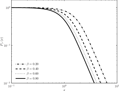
(a)    CCDF for some different values of $\beta$

(b)    PDF for some different values of $\beta$

Figure 1: 1(a) Plot of the $\kappa$-generalized CCDF given by Eq. (II.1) versus $x$ for some different values of $\beta$ ($=0.20,0.40,0.60,0.80$), and fixed $\alpha$ ($=2.50$) and $\kappa$ ($=0.75$). 1(b) Plot of the $\kappa$-generalized PDF given by Eq. (II.4) versus $x$ for some different values of $\beta$ ($=0.20,0.40,0.60,0.80$), and fixed $\alpha$ ($=2.50$) and $\kappa$ ($=0.75$). Notice that the distribution spreads out (concentrates) as the value of $\beta$ decreases (increases)

The exponent $\alpha>0$ quantifies the curvature (shape) of the distribution, which is less (more) pronounced for lower (higher) values of the parameter, as seen in FIG. 2(a)–2(b).

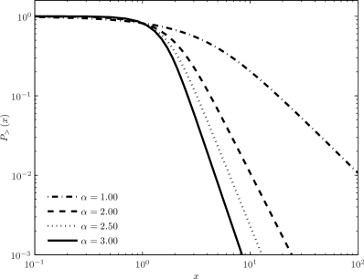
(a)    CCDF for some different values of $\alpha$

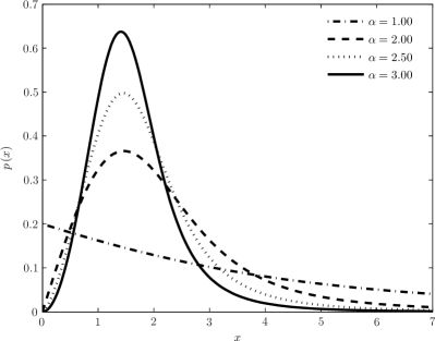
(b)    PDF for some different values of $\alpha$

Figure 2: 2(a) Plot of the $\kappa$-generalized CCDF given by Eq. (II.1) versus $x$ for some different values of $\alpha$ ($=1.00,2.00,2.50,3.00$), and fixed $\beta$ ($=0.20$) and $\kappa$ ($=0.75$). 2(b) Plot of the $\kappa$-generalized PDF given by Eq. (II.4) versus $x$ for some different values of $\alpha$ ($=1.00,2.00,2.50,3.00$), and fixed $\beta$ ($=0.20$) and $\kappa$ ($=0.75$). Notice that the curvature (shape) of the distribution becomes less (more) pronounced when the value of $\alpha$ decreases (increases). The case $\alpha=1.00$ corresponds to the ordinary exponential function

Finally, as one can observe in FIG. 3(a)–3(b), the deformation parameter $\kappa\in\left[0,1\right)$ measures the fatness of the upper tail: the larger (smaller) its magnitude, the fatter (thinner) the tail.

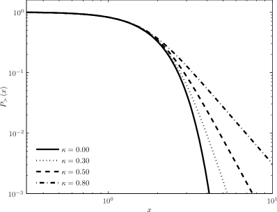
(a)    CCDF for some different values of $\kappa$

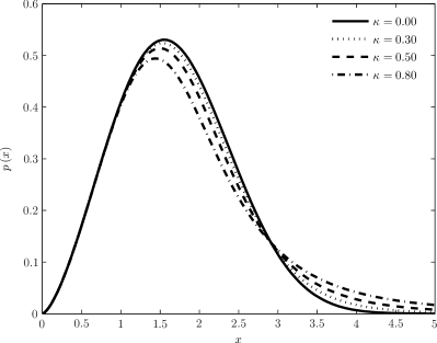
(b)    PDF for some different values of $\kappa$

Figure 3: 3(a) Plot of the $\kappa$-generalized CCDF given by Eq. (II.1) versus $x$ for some different values of $\kappa$ ($=0.00,0.30,0.50,0.80$), and fixed $\beta$ ($=0.20$) and $\alpha$ ($=2.50$). 3(b) Plot of the $\kappa$-generalized PDF given by Eq. (II.4) versus $x$ for some different values of $\kappa$ ($=0.00,0.30,0.50,0.80$), and fixed $\beta$ ($=0.20$) and $\alpha$ ($=2.50$). Notice that the upper tail of the distribution fattens (thins) as the value of $\kappa$ increases (decreases). The case $\kappa=0.00$ corresponds to the ordinary stretched exponential (Weibull) function LaherrereSornette1998 ; Sornette2000

The function $P_{>}\left(x\right)$ defined through Eq. (II.1) can be viewed as a generalization of the ordinary stretched exponential LaherrereSornette1998 , i.e. $P_{>}^{0}\left(x\right)=\exp\left(-\beta x^{\alpha}\right)$, which recovers in the $\kappa\rightarrow 0$ limit. It is remarkable that $P_{>}\left(x\right)$ for $x\rightarrow 0^{+}$ behaves as the ordinary stretched exponential

$$P_{>}\left(x\right){\atop\stackrel{{\scriptstyle\textstyle\sim}}{{\scriptstyle x\rightarrow{0^{+}}}}}\exp\left(-\beta x^{\alpha}\right),$$ (II.2)

while for $x\rightarrow\infty$ presents a power-law tail

$$P_{>}\left(x\right){\atop\stackrel{{\scriptstyle\textstyle\sim}}{{\scriptstyle x\rightarrow{+\infty}}}}\left(2\beta\kappa\right)^{-1/\kappa}x^{-\alpha/\kappa}.$$ (II.3)

The Probability Density Function (PDF), $p\left(x\right)=-\mathrm{d}P_{>}\left(x\right)/\mathrm{d}x$, is given by

$$p\left(x\right)=\frac{\alpha\beta x^{\alpha-1}\exp_{\kappa}\left(-\beta x^{\alpha}\right)}{\sqrt{1+\beta^{2}\kappa^{2}x^{2\alpha}}},$$ (II.4)

and can viewed as a generalization of the Weibull distribution Sornette2000 , i.e. $p^{0}\left(x\right)=\alpha\beta x^{\alpha-1}\exp\left(-\beta x^{\alpha}\right)$, which recovers in the $\kappa\rightarrow 0$ limit. The function $p\left(x\right)$ given by Eq. (II.4) for $x\rightarrow 0^{+}$ behaves as a Weibull distribution

$$p\left(x\right){\atop\stackrel{{\scriptstyle\textstyle\sim}}{{\scriptstyle x\rightarrow{0^{+}}}}}\alpha\beta x^{\alpha-1}\exp\left(-\beta x^{\alpha}\right),$$ (II.5)

while for $x\rightarrow+\infty$ reduces to the Pareto’s law

$$p\left(x\right){\atop\stackrel{{\scriptstyle\textstyle\sim}}{{\scriptstyle x\rightarrow{+\infty}}}}\frac{\alpha}{\kappa}\left(2\beta\kappa\right)^{-1/\kappa}x^{-\left(\frac{\alpha}{\kappa}+1\right)}.$$ (II.6)

Starting from the law (II.4), one can calculate the mean value $\left\langle x\right\rangle$ which, taking into account the meaning of the variable $x$, results to be equal to unity

$$\int\limits_{0}^{\infty}xp\left(x\right)\mathrm{d}x=1.$$ (II.7)

The latter relationship permits to express the parameter $\beta$ as a function of the parameters $\kappa$ and $\alpha$, obtaining

$$\beta=\frac{1}{2\left|\kappa\right|}\left[\frac{\Gamma\left(\frac{1}{\alpha}\right)}{\left|\kappa\right|+\alpha}\frac{\Gamma\left(\frac{1}{2|\kappa|}-\frac{1}{2\alpha}\right)}{\Gamma\left(\frac{1}{2|\kappa|}+\frac{1}{2\alpha}\right)}\right]^{\alpha},$$ (II.8)

where $\Gamma\left(x\right)$ is the Euler gamma function $\Gamma\left(x\right)=\int_{0}^{\infty}t^{x-1}e^{-t}\mathrm{d}t$. Thus the problem to determine the values of the free parameters ($\kappa$, $\alpha$, $\beta$) of the theory from the empirical data reduces to a two parameter ($\kappa$, $\alpha$) fitting problem.

III An application to personal income data

As a working example, we analyze the census data on personal income in three countries: Germany, Italy, and the United Kingdom.

The data used are drawn primarily from the Cross-National Equivalent File (CNEF) 1980–2002, a commercially available dataset compiled by researchers at Cornell University which attempts to make comparable, among others, the following panel surveys: the German Socio-Economic Panel (GSOEP) and the British Household Panel Study (BHPS). The income variable we use is the post-government income, representing the combined income after taxes and government transfers of the head, partner, and other family members.

For Italy, which is not part of the CNEF, we use the Survey on Household Income and Wealth (SHIW), a household-based panel study carried out by the Bank of Italy since 1977. In place of the post-government income in the CNEF, we use the net disposable income variable from the survey above—i.e., the income recorded after the payment of taxes and social security contributions, defined as the sum of four main components: compensation of employees, pensions and net transfers, net income from self-employment, and property income.

The results obtained by fitting our theoretical model through the observational data are reported in TABLE 1 and FIGS. 4, 5, and 6. Panel (a) of the figures shows the empirical cumulative distribution estimate of $x$ along with three different curves in the log-log scale: the $\kappa$-generalized distribution, Eq. (II.1); the ordinary stretched exponential (Weibull) distribution, Eq. (II.2); the pure power-law distribution, Eq. (II.3). In panel (b), the histogram of the reconstructed probability density is contrasted to the theoretical curves corresponding to Eqs. (II.4) and (II.5) with the same parameter values as in TABLE 1 and panel (a) of FIGS. 4, 5, and 6. It is clear that the $\kappa$-generalized distribution offers a great potential for describing the data over their whole range, from the low to medium income region through to the high income Pareto power-law regime, including the intermediate region for which a clear deviation exists when two different curves are used.

Table 1: Estimated parameters (with 95% confidence intervals half-widths) of the $\kappa$-generalized distribution for the countries and years shown in FIGS. 4, 5, and 6. Also shown is the estimated weighted average income

	Germany	Italy	United Kingdom
$\kappa$	$0.5697\pm 0.0005$	$0.6944\pm 0.0006$	$0.7080\pm 0.0006$
$\alpha$	$2.5659\pm 0.0007$	$2.2540\pm 0.0007$	$2.7357\pm 0.0009$
$\beta$	$0.8788\pm 0.0003$	$1.0087\pm 0.0004$	$0.9433\pm 0.0004$
$\left\langle z\right\rangle$	$36315.67\pm 339.24$	$18087.92\pm 246.85$	$14982.20\pm 183.09$

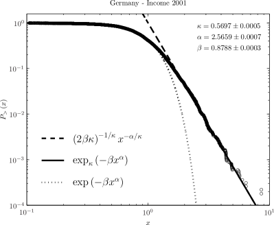
(a)    Complementary CDF

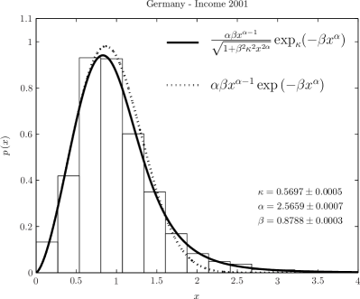
(b)    PDF histogram plot

Figure 4: The German personal income distribution from the 2001 GSOEP-CNEF data file measured in current year euros. 4(a) Plot of the empirical CCDF versus income in the log-log scale. The solid line is our theoretical model given by Eq. (II.1) with $\kappa=0.5697\pm 0.0005$, $\alpha=2.5659\pm 0.0007$, and $\beta=0.8788\pm 0.0003$, which fits very well the data in the whole range from the low to the high incomes including the intermediate income region. This function is compared with the ordinary stretched exponential one (dotted line)—fitting the low income data—and with the pure power-law (dashed line)—fitting the high income data—by using the same parameter values. 4(b) Histogram plot of the empirical PDF with superimposed fits of the $\kappa$-generalized (solid line) and stretched exponential (dotted line) PDFs using the same parameter values as in panel 4(a). The income axis limits have been adjusted according to the range of data to shed light on the intermediate region between the bulk and the tail of the distribution

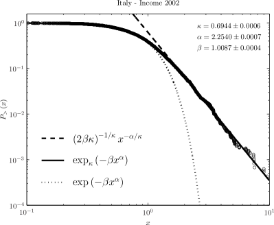
(a)    Complementary CDF

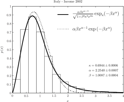
(b)    PDF histogram plot

Figure 5: Same plots as in FIG. 4 for the Italian personal income distribution from the 2002 SHIW data file with $\kappa=0.6944\pm 0.0006$, $\alpha=2.2540\pm 0.0007$, and $\beta=1.0087\pm 0.0004$. The income variable is measured in current year euros

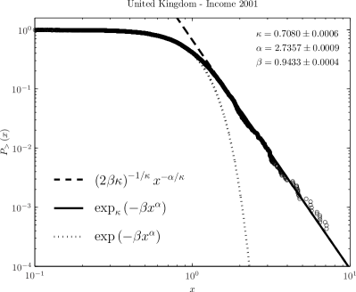
(a)    Complementary CDF

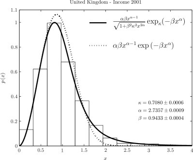
(b)    PDF histogram plot

Figure 6: Same plots as in FIGS. 4 and 5 for the UK personal income distribution from the 2001 BHPS-CNEF data file with $\kappa=0.7080\pm 0.0006$, $\alpha=2.7357\pm 0.0009$, and $\beta=0.9433\pm 0.0004$. The income variable is measured in current year British pounds

IV Final remarks

Since the early study of Pareto, numerous recent empirical works have all shown that the power-law tail is an ubiquitous feature of income distributions. However, even 100 years after Pareto’s observation, the understanding of the shape of income distribution is still far to be complete and definitive. This reflects the fact that there are two distributions, one for the rich, following the Pareto’s law, and one for the vast majority of people, which appears to be governed by a completely different law.

In the present work we have affirmed support for a new fitting function, having its roots in the framework of $\kappa$-generalized statistical mechanics, which shows to be able to describe the data over the entire range, including even the power-law tail. This distribution has a bulk very close to the stretched exponential one—which is recovered when the deformation parameter $\kappa$ approaches to zero—while its tail decays following a power-law for high values of income, thus providing a kind of compromise between the two description.

The good concordance of our generalized statistical distribution with observational data on personal income may suggest a new path for investigating economic relations, namely the development of models within the framework of $\kappa$-generalized statistical mechanics.

References

- (1) Chatterjee, A., Yarlagadda, S., and Chakrabarti, B. K. (2005). Econophysics of Wealth Distributions. Milan: Springer-Verlag Italia.
- (2) Richmond, P., Hutzler, S., Coelho, R., and Repetowicz, P., (2006). A review of empirical studies and models of income distributions in society. In B. K. Chakrabarti, A. Chakraborti, and A. Chatterjee (Eds.), Econophysics and Sociophysics: Trends and Perspectives (pp. 131–160). Berlin: Wiley-VCH.
- (3) Pareto, V. (1896). La courbe de la reṕartition de la richesse. Reprinted 1965 in G. Busoni (Ed.), Œeuvres complètes de Vilfredo Pareto, Tome 3: Écrits sur la courbe de la répartition de la richesse, Geneva: Librairie Droz. English translation in Rivista di Politica Economica, 87 (1997), 647–700.
- (4) Pareto, V. (1897a). Course d’économie politique. London: Macmillan.
- (5) Pareto, V. (1897b). Aggiunta allo studio della curva delle entrate. Giornale degli Economisti, 14, 15–26. English translation in Rivista di Politica Economica, 87 (1997), 645–700.
- (6) Arnold, B. C. (1983). Pareto Distributions. Fairland: International Co-operative Publishing House.
- (7) Gibrat, R. (1931). Les inégalités économiques. Applications: aux inégalités des richesses, à la concentration des entreprises, aux populations des villes, etc., d’une loi nouvelle: la loi de l’effet proportionel. Paris: Librairie du Recueil Sirey.
- (8) Aitchison, J., and Brown, J. A. C. (1954). On criteria for description of income distribution. Metroeconomica, 6, 88- 107.
- (9) Aitchison, J., and Brown, J. A. C. (1957). The Lognormal Distribution with Special Reference to its Use in Economics. Cambridge: Cambridge University Press.
- (10) Montroll, E. W., and Shlesinger, M. F. (1982). On noise and other distributions with long tails. Proceedings of the National Academy of Sciences USA, 79, 3380- 3383.
- (11) Montroll, E. W., and Shlesinger, M. F. (1983). Maximum entropy formalism, fractals, scaling phenomena, and noise: A tale of tails. Journal of Statistical Physics, 32, 209- 230.
- (12) Souma, W. (2001). Universal structure of the personal income distribution. Fractals, 9, 463- 470.
- (13) Di Matteo, T., Aste, T., and Hyde, S. T. (2004). Exchanges in complex networks: Income and wealth distributions. In F. Mallamace and H. E. Stanley (Eds.), The Physics of Complex Systems (New Advances and Perspectives) (pp. 435- 442). Amsterdam: IOS Press.
- (14) Clementi, F., and Gallegati, M. (2005a). Power law tails in the Italian personal income distribution. Physica A: Statistical and Theoretical Physics, 350, 427–438.
- (15) Clementi, F., and Gallegati, M. (2005b). Pareto’s law of income distribution: Evidence for Germany, the United Kingdom, and the United States. In A. Chatterjee, S. Yarlagadda, and B. K. Chakrabarti (Eds.), Econophysics of Wealth Distributions (pp. 3- 14). Milan: Springer-Verlag Italia.
- (16) Drăgulescu, A. A., and Yakovenko, V. M. (2001a). Evidence for the exponential distribution of income in the USA. The European Physical Journal B, 20, 585- 589.
- (17) Drăgulescu, A. A., and Yakovenko, V. M. (2001b). Exponential and power-law probability distributions of wealth and income in the United Kingdom and the United States. Physica A: Statistical Mechanics and its Applications, 299, 213- 221.
- (18) Nirei, M., and Souma, W. (2004). Two factor model of income distribution dynamics. SFI Working Paper No. 04-10-029. Available at: http://www.santafe.edu/research/publications/wpabstract/200410029.
- (19) Willis, G., and Mimkes, J. (2004). Evidence for the independence of waged and unwaged income, evidence for Boltzmann distributions in waged income, and the outlines of a coherent theory of income distribution. EconWPA No. 0408001. Available at: http://ideas.repec.org/p/wpa/wuwpmi/0408001.html.
- (20) Silva, A. C., and Yakovenko, V. M. (2005). Temporal evolution of the “thermal” and “superthermal” income classes in the USA during 1983- 2001. Europhysics Letters, 69, 304- 310.
- (21) Kaniadakis, G. (2001a). Non-linear kinetics underlying generalized statistics. Physica A: Statistical Mechanics and its Applications, 296, 405- 425.
- (22) Kaniadakis, G. (2001b). H-theorem and generalized entropies within the framework of nonlinear kinetics. Physics Letters A, 288, 283–291.
- (23) Kaniadakis, G. (2002). Statistical mechanics in the context of special relativity. Physical Review E, 66, 56125.
- (24) Kaniadakis, G. (2005). Statistical mechanics in the context of special relativity. II. Physical Review E, 72, 36108.
- (25) Kaniadakis, G. (2006). Towards a relativistic statistical theory. Physica A: Statistical Mechanics and its Applications, 365, 17–23.
- (26) Laherrère, J., and Sornette, D. (1998). Stretched exponential distributions in nature and economy: fat tails with characteristic scales. Europen Physical Journal B, 2, 525–539.
- (27) Sornette, D. (2000). Critical Phenomena in Natural Sciences. Chaos, Fractals, Selforganization and Disorder: Concepts and Tools. Heidelberg: Springer-Verlag Berlin.
- (28) Clementi, F., Di Matteo, T., and Gallegati, M. (2006). The power-law tail exponent of income distributions. Physica A: Statistical and Theoretical Physics, 370, 49- 53.
- (29) Burkhauser, R. V., Butrica, B. A., Daly, M. C., and Lillard, D. R. (2001). The Cross-National Equivalent File: A product of cross-national research. In I. Becker, N. Ott, and G. Rolf (Eds.), Soziale Sicherung in einer dynamischen Gesellschaft. Festschrift für Richard Hauser zum 65 (Social Insurance in a Dynamic Society. Papers in Honor of the 65th Birthday of Richard Hauser) (pp. 354 -76). Frankfurt and New York: Geburtstag Campus. Available at: http://www.human.cornell.edu/che/PAM/Research/Centers-Programs/German-Panel/upload/P25-2.PDF.
- (30) Brandolini, A. (1999). The distribution of personal income in post-war Italy: Source description, data quality, and the time pattern of income inequality. Temi di discussione (Economic working papers) from Bank of Italy No. 350. Available at: http://www.bancaditalia.it/ricerca/consultazioni/temidi/td99/tema_350_99.pdf.
- (31) Schoenberg, R. (1997). Constrained maximum likelihood. Computational Economics, 10, 251–266.
- (32) Expert Group on Household Income Statistics—The Canberra Group (2001). Final report and recommendations. Available at: http://www.lisproject.org/links/canberra/finalreport.pdf.
- (33) Han, S. P. (1977). A globally convergent method for nonlinear programming. Journal of Optimization Theory and Applications, 22, 297–309.
- (34) Kleiber, C., and Kotz, S. (2003). Statistical Size Distributions in Economics and Actuarial Sciences. New York: John Wiley & Sons.