Complexity analysis of the stock market

Abstract

We study the complexity of the stock market by constructing $\epsilon$-machines of Standard and Poor’s 500 index from February 1983 to April 2006 and by measuring the statistical complexities. It is found that both the statistical complexity and the number of causal states of constructed $\epsilon$-machines have decreased for last twenty years and that the average memory length needed to predict the future optimally has become shorter. These results support that the information is delivered to the economic agents and applied to the market prices more rapidly in year 2006 than in year 1983.

1 Introduction

Financial systems have been one of active research fields for physicists. This interdisciplinary research area called econophysics has been investigated by means of various statistical methods, such as the correlation function, multifractality, minimal spanning tree, minority games, continuous-time random walks, and spin models [1, 2, 3, 4, 5, 6, 7, 8, 9]. Recently many empirical time series in financial markets become available and has been also investigated by the rescaled range (R/S) analysis to test the presence of correlations [10] and detrended fluctuation analysis to detect long-range correlations embedded in seemingly non-stationary time series [11, 12] and so on.

In this paper we adopt the computational mechanics (CM) [13, 14] to investigate the complexity of the stock market. The CM is based on the early works of the information and computation theory done by Shannon, Kolmogorov, and Chaitin [15, 16, 17]. Despite its strong functionality, CM has been applied only to analyze the abstract models such as cellular automata [18, 19] and Ising spin system [20], or empirical data in the geomagnetism [21] and in the atmosphere [22]. We believe that CM enables the complexities and structures of different sets of data to be quantifiably compared and that it directly discovers intrinsic causal structure within the data [21]. This approach also shows how to infer a model of the hidden process that generated the observed behavior.

We examined the tick data of Standard and Poor’s 500 (S&P500) index from February 1983 to April 2006 by constructing deterministic finite automata called “epsilon-machine” [23] from the financial time series and by calculating the statistical complexity from the constructed machine. The $\epsilon$-machine captures the patterns and regularities in the observations in a way that reflects the causal structure of the process. With this model in hand, we can extrapolate beyond the original observations to predict future behavior [14]. The constructed $\epsilon$-machine is a step toward the eventual use of such machine in finding effective patterns embedded in the price index of stock market. This is a novel approach to predict the next action on the stock market with statistical probabilities. We also analyzed the result that the complexity of the stock market has decreased.

2 Principles

According to Feldman [13] and Shailizi [14] we introduce the basics regarding to the $\epsilon$-machine and the statistical complexity as complexity measure.

2.1 $\epsilon$-machine

We consider a stochastic process given by an infinitely consecutive discrete random variables, $\overleftrightarrow{X}=\cdots X_{-1}X_{0}X_{1}X_{2}\cdots$, where each $X_{i}$ may take a symbol $x_{i}$ drawn from a finite countable set $A$ of size $k$. At any time $t$ this sequence of random variables can be divided into two semi-infinite halves; a history $\overleftarrow{X_{t}}$ and a future $\overrightarrow{X_{t}}$. If the process is conditionally stationary, i.e. for all possible future events $F$, $\Pr(\overrightarrow{X_{t}}\in F\mid\overleftarrow{X_{t}}=\overleftarrow{x})$ does not depend on $t$, then we drop the subscript. And $\overrightarrow{X^{l}}$ and $\overleftarrow{X^{l}}$ denote the first $l$ variables of $\overrightarrow{X}$ and the last $l$ variables of $\overleftarrow{X}$, respectively.

A causal state is defined as a set of history events (shortly, histories) that have the same distribution of conditional probabilities for all possible future events. $\epsilon$ is a function that maps from histories to sets of histories:

$$\epsilon(\overleftarrow{x})=\{\overleftarrow{x^{\prime}}\mid\Pr(\overrightarrow{X}=\overrightarrow{x}\mid\overleftarrow{X}=\overleftarrow{x})=\Pr(\overrightarrow{X}=\overrightarrow{x}\mid\overleftarrow{X}=\overleftarrow{x^{\prime}}),\forall\overrightarrow{x}\in F\}.$$ (1)

Each causal state $s_{i}$ consists of its name $i$, a set of histories $\epsilon(\overleftarrow{x})$, and the conditional probability distribution $\Pr(\overrightarrow{X}\in F\mid\overleftarrow{X}=\overleftarrow{x})$, which is called “morph.” $S$ denotes the corresponding random variable and $\mathbb{S}$ does the set of all causal states. Then, the transition probability $T_{ij}^{(a)}$ is defined as the probability of generating a symbol $a\in A$ when making the transition from state $s_{i}$ to state $s_{j}$;

$$T_{ij}^{(a)}\equiv\Pr(\overleftarrow{X}a\in s_{j}\mid\overleftarrow{X}\in s_{i}),$$ (2)

where $\overleftarrow{X}a$ is read as a semi-infinite sequence obtained by concatenating $a\in A$ onto the end of $\overleftarrow{X}$. Equivalently,

$$T_{ij}^{(a)}=\Pr(S^{\prime}=s_{j},\overrightarrow{X^{1}}=a\mid S=s_{i}),$$ (3)

where $S$ and $S^{\prime}$ are random variables for the current causal state and its successor, respectively. The combination of the function $\epsilon$ mapping from histories to causal states with the labeled transition probabilities $T_{ij}^{(a)}$ is called the $\epsilon$-machine, which represents a computational model underlying the given time series. The causal states and the transitions of $\epsilon$-machine form a directed graph, therefore there can exist some states being never returned once the system left those states. These are called transient states that cannot be the true causal states so removed and the others are recurrent states [24]. Once the $\epsilon$-machine is constructed and the current causal state is identified, one can optimally predict the future behavior of the process with some conditional probability distributions, which will be useful in practice, for example, for traders in financial markets.

For the operational applications the length of histories to be considered is limited as $L_{\textrm{max}}$ for a process with finitely consecutive random variables or finite time series. $L_{\textrm{max}}$ should be large enough to fully detect the structure embedded in the process. On the other hand it is also limited by the total number $N$ of data points available in a way of $L_{\textrm{max}}<\log_{k}N$ [24] for the significant analysis.

2.2 Statistical and topological complexities

From the constructed $\epsilon$-machine, for each $i$ the probability of finding the system in the $i$-th causal state after the machine has been running infinitely long, $\Pr(s_{i})$, can be calculated. The components $T_{ij}$ of the transition matrix $T=\sum_{a\in A}T_{ij}^{(a)}$ gives the probability of a transition from state $s_{i}$ to state $s_{j}$. $\Pr(s_{i})$ are obtained by solving the following:

$$\sum_{i}\Pr(s_{i})T_{ij}=\Pr(s_{j}).$$ (4)

Then the statistical and topological complexities are defined as

$$C_{\mu}\equiv-\sum_{i}\Pr(s_{i})\log_{2}\Pr(s_{i}),$$ (5)

$$C_{0}\equiv\log_{2}\|\mathbb{S}\|,$$ (6)

where $\|\cdot\|$ represents the cardinality of a set. $C_{\mu}$ measures the minimum amount of historical information required to make optimal forecasts [20, 22]. By the definitions of the statistical and topological complexities, the topological complexity is the upper bound of the statistical complexity. And the equality holds when the distribution is uniform, that is, for all causal states $\Pr(s_{i})=1/\|\mathbb{S}\|$. As the probability distribution of causal states deviate from uniformity, the statistical complexity becomes smaller and therefore far from the topological complexity.

2.3 Simple examples

Before closing this section, a few simplest examples are examined by constructing the $\epsilon$-machines. The first is a process generating the same symbol infinitely, such as $\cdots 000\cdots$. There exists the only one causal state consisting of the only one history $\overleftarrow{x}=\cdots 000$ and the morph $\Pr(0\mid\overleftarrow{x})=1$. If we depict each causal state as a node and each transition from state $i$ to $j$ generating a symbol $a$ with probability $p$ as an arc starting from a node $i$ to $j$ on which ‘$a\mid p$’ is labeled, then the above $\epsilon$-machine would be depicted as one node and one arc going back to itself with ‘$0\mid 1$’ labeled. In this case both complexities of Eqs. (5-6) become $0$ bit.

The second example is a periodic series with period $2$, such as $\cdots 0101\cdots$. Two histories are found: $\overleftarrow{x_{1}}=\cdots 101$, $\overleftarrow{x_{2}}=\cdots 010$. Since $\Pr(0\mid\overleftarrow{x_{1}})=1$ while $\Pr(0\mid\overleftarrow{x_{2}})=0$, each histories constitutes each causal state. The constructed $\epsilon$-machine consists of two nodes and two arcs coming from one circle to the other, respectively. In this case both complexities of Eqs. (5-6) become $1$ bit.

As the final one we toss a fair coin and record $H$ for head, $T$ for tail, and get a random process such as $\cdots HHTHT\cdots$. There are infinitely many histories but all the morphs are the same as $\Pr(H\mid\overleftarrow{x_{i}})=\Pr(T\mid\overleftarrow{x_{i}})=1/2$. Therefore the only one causal state is enough for the $\epsilon$-machine, which consists of one node and two arcs going back to itself but with different labels, ‘$H\mid 1/2$’ and ‘$T\mid 1/2$’, respectively. Both complexities of Eqs. (5-6) become $0$ bit, which means the totally random process is not complex at all. Thus, these measures satisfy the so-called ‘boundary condition’ for the complexity measure that vanishes in the extreme ordered and disordered limits [25].

3 Empirical data analysis

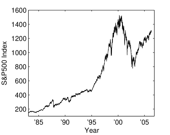
Figure 1: The time series of S&P500 index from February 1983 to April 2006.

For the tick-by-tick S&P500 index data from February 1983 to April 2006, as shown in Fig. 1, the statistical and topological complexities are calculated from constructed $\epsilon$-machines [26]. By using a time window of one year and shifting the window by one month, we get $267$ data sets and for each data set each $\epsilon$-machine is constructed. For convenience each data set is named after its starting month, for example, the data set for one year since February 1983 is called February 1983 data. The average number of data points in one minute varies from about $1$ in the early 1980’s to $4$ in recent years. For the analysis we firstly set a countable set $A$ to the smallest set of size $k=2$, such as $\{0,1\}$. Then the original index data $Y_{n}$ change into the binary time series $F_{n}$ by the following process:

$$F_{n}\equiv\theta\left(Y_{n+1}-Y_{n}\right),$$ (7)

where $\theta(x)$ is a Heaviside step function. $F_{n}$ gets the value of $0$ if the next index has decreased and does the value of $1$ otherwise. Since New York Stock Exchange opens during the day time, we use only the intra-day data to avoid the discontinuous jump between the previous day’s closing index and the next day’s opening index due to overnight effects. In other words we exclude $F_{n}$ for the difference between the last index of the previous day and the first index of the next day.

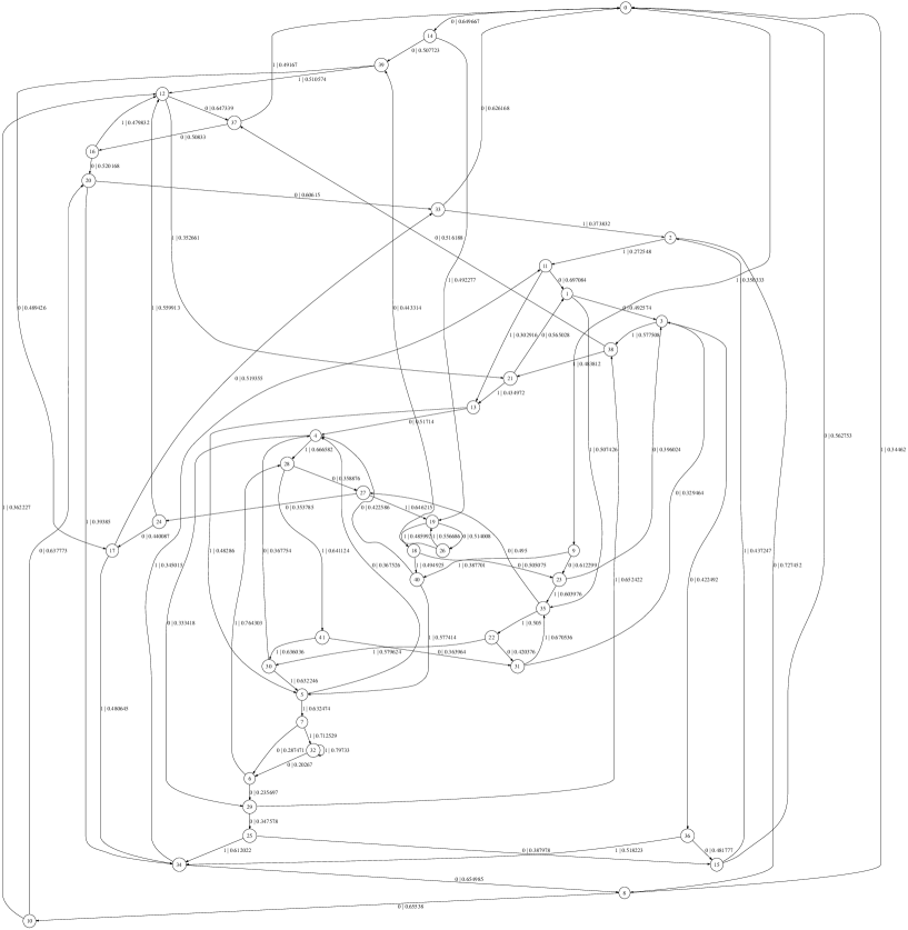
Figure 2: The $\epsilon$-machine constructed from the February 1983 data of S&P500 index. The figure has been produced with the Graphviz software (http://www.graphviz.org/).

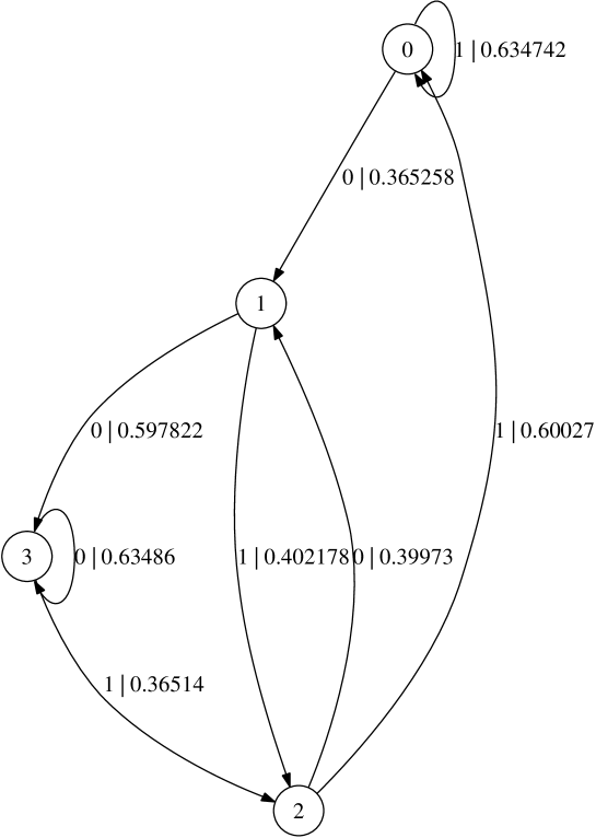
Figure 3: The $\epsilon$-machine constructed from the April 2005 data of S&P500 index. The figure has been produced with the Graphviz software.

To construct $\epsilon$-machines we set $L_{\textrm{max}}$ to $6$, which gives the most reliable results. Figures 2 and 3 depict the $\epsilon$-machines for the February 1983 data and for the April 2005 data, respectively. It is noteworthy that the number of causal states has decreased for last twenty years, which will be discussed later. In those figures, as mentioned, each numbered node represents a causal state, while each arc joining one node to another does the transition from one causal state to another. Each arc is labeled with ‘$a\mid p$’, that is, a symbol $a$ is generated with probability $p$ by that transition. For example, in Fig. 3 if the current state of the system is the $0$th one, the system goes back to the $0$th state by generating symbol $1$ with probability $p=0.634742$, while the system makes a transition to the $1$st state by generating symbol $0$ with probability $1-p$. The directions of these arcs tell us which causal state will be followed.

In more details, we investigate the histories belonging to each causal state. The histories of each causal state for two $\epsilon$-machines mentioned before are shown in Tables 1 and 2, respectively. Since we set the length of the longest histories to be considered as $6$, there are $2^{6}=64$ possible histories of length $6$. In particular the histories of the $0$th causal state in Fig. 3 can be found in the first row of Table 2. If we add symbol $1$ on the right end of each history and limit the length to $6$ (e.g., $000011\rightarrow 000111$), we can see that all the resulting histories remain included in the $0$th causal state. For the opposite case of adding symbol $0$ on the right end (e.g., $000011\rightarrow 000110$), all the resulting histories are found in the $1$st causal state. By making use of this method repeatedly as we want, we can predict the next finitely consecutive symbols with a certain probability, which can be obtained just by multiplying the transition probabilities along the arcs.

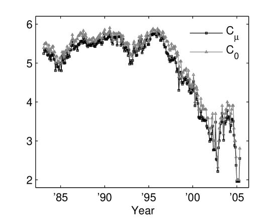
Figure 4: The decreasing behaviors of the statistical complexity $C_{\mu}$ and the topological complexity $C_{0}$ of S&P500 index from February 1983 to April 2006. Notice that $C_{0}$ is upper bound of $C_{\mu}$.

Next, we found that both the statistical and topological complexities of S&P500 index have a tendency of decreasing through time as shown in Fig. 4. Since the time window is set to one year, it is assumed that many short term events in the stock market, such as the Black Monday, do not affect our analysis. Therefore we focus on the long term behaviors of both complexities. Since the difference between the statistical and topological complexities is not significant for the whole range of times, the probability distributions for causal states are almost uniform throughout time. Conclusively our main concern is reduced to the decrease in the number of causal states. Precisely, the total number of causal states decreases from $42$ for the February 1983 data to $4$ for the April 2005 data.

To find the underlying principle of the decrease in the number of causal states through time, we revisit Tables 1 and 2 showing the histories of length $L=6$ of the causal states for the February 1983 and April 2005 data, respectively. In Table 1 the $62$ histories are mapped to $42$ causal states according to their morphs (the other $2$ histories were in the removed transient states) and thus the causal states are composed of only one to three histories. It is found that for each causal state with two histories each two histories are the same except the left end symbols of them, that is, $L=5$ is enough to identify such states. But for the majority of causal states $L=6$ is necessary. Therefore it is reasonable to conclude that the average memory length we need to predict the future at the February 1983 data was $6$, which corresponds to about $6$ minutes.

In Table 2, the causal states for the April 2005 data are more simplified than the above case. $64$ histories are grouped into $4$ causal states exactly containing $16$ histories, respectively. In each causal state all the histories have the last two symbols in common; $11$ for the $0$th causal state and $10$ for the $1$st one and so on. The first $4$ symbols of each history are all the possible matches of $0$’s and $1$’s. In this case the average memory length to predict the future for the April 2005 data was $2$, i.e. about one half minute. In conclusion, the average memory length needed to predict the future has decreased from $6$ in the early 1980’s to $2$ in recent years.

Now the decreasing tendency of statistical and topological complexities for last twenty years is explained. We call the common part of histories in each causal state an ‘effective pattern.’ If the length of effective pattern $L_{\textrm{eff}}$ decreases, the number of possible effective patterns decreases as $2^{L_{\textrm{eff}}}$, so does that of the resultant causal states. Although we had set $L_{\textrm{max}}$ to $6$ for the entire range of time, $L_{\textrm{eff}}$ decreased from $6$ to $2$ in recent years. Since only effective patterns affect the identification of causal states and transitions among them, they contribute to predict the future and also can be interpreted as the correlation interval. Therefore, in the early 1980’s one had to look back $6$ ticks for the prediction of the next tick index, that is, about $6$ consecutive tick indices are correlated. On the other hand in recent years, one only need to look back $2$ ticks for the prediction, which means the shorter correlation than before.

The correlation interval is closely related to the time scale for new information to be delivered to the economic agents and applied to the market prices [27, 28]. The decreasing correlation interval for last twenty years supports that the information flows faster than before and that the memory length for the optimal prediction becomes smaller.

4 Conclusions

In this paper, we investigated the S&P500 index from February 1983 to April 2006 by constructing $\epsilon$-machines to infer the hidden causal structures embedded in the data and by measuring the statistical and topological complexities from the $\epsilon$-machines. If in the constructed causal structure the current causal state is identified, then by following the path from state to state one can predict the future behavior of a finite interval. This would be useful in practice, for example, for traders in financial markets.

We also found that the statistical complexity and the number of causal states of constructed $\epsilon$-machines have decreased for last twenty years. Precisely, the length of effective patterns in histories has become shorter in recent years than in the early 1980’s. These results imply that the information flows faster and hence the memory length needed to predict the future optimally has become shorter.

Causal state	Histories $\overleftarrow{x}$	Morph	Causal state	Histories $\overleftarrow{x}$	Morph
name		$\Pr(1\mid\overleftarrow{x})$	name		$\Pr(1\mid\overleftarrow{x})$
0	000101 100101	0.350333	20	001000	0.39385
	100000		21	010011 110011	0.434972
1	000110 100110	0.507426	22	011011	0.579624
2	100001	0.272548	23	010110	0.603976
3	001100 101100	0.577508	24	110100	0.559913
4	001110 011110	0.666582	25	111000	0.612022
	101110		26	101010	0.556686
5	001111 101111	0.632474	27	011010 111010	0.646215
6	111110	0.764303	28	011101 111101	0.641124
7	011111	0.712529	29	011100 111100	0.652422
8	000010 100010	0.34462	30	110111	0.632246
9	001011	0.387701	31	110110	0.670536
10	000100	0.362227	32	111111	0.79733
11	000011 100011	0.302916	33	010000	0.373832
12	001001 101001	0.352661	34	010001 110001	0.345015
13	000111 100111	0.48286	35	001101 101101	0.505
14	001010	0.492277	36	011000	0.518223
15	110000	0.437247	37	010010 110010	0.49167
16	100100	0.479832	38	011001 111001	0.483812
17	101000	0.480645	39	010100	0.510574
18	101011	0.494925	40	010111	0.577414
19	010101 110101	0.485992	41	111011	0.636036

Table 1: The causal states of $\epsilon$-machine constructed from the February 1983 data. Each causal state consists of its name, histories, and morph.

Causal state	Histories $\overleftarrow{x}$	Morph	Causal state	Histories $\overleftarrow{x}$	Morph
name		$\Pr(1\mid\overleftarrow{x})$	name		$\Pr(1\mid\overleftarrow{x})$
0	000011 100011	0.634742	2	000001 100001	0.60027
	000111 100111			000101 100101
	001011 101011			001001 101001
	001111 101111			001101 101101
	010011 110011			010001 110001
	010111 110111			010101 110101
	011011 111011			011001 111001
	011111 111111			011101 111101
1	000010 100010	0.402178	3	000000 100000	0.36514
	000110 100110			000100 100100
	001010 101010			001000 101000
	001110 101110			001100 101100
	010010 110010			010000 110000
	010110 110110			010100 110100
	011010 111010			011000 111000
	011110 111110			011100 111100

Table 2: The causal states of $\epsilon$-machine constructed from the April 2005 data.

References

- [1] W. B. Arthur, S. N. Durlauf, D. A. Lane (Eds.), The Economy as an Evolving Complex System II, Perseus Books, 1997.
- [2] R. N. Mantegna, H. E. Stanley, An Introduction to Econophysics: Correlations and Complexity in Finance, Cambridge University Press, 2000.
- [3] J.-P. Bouchaud, M. Potters, Theory of Financial Risks: From Statistical Physics to Risk Management, Cambridge University Press, 2000.
- [4] B. B. Mandelbrot, Quant. Finance 1 (2001) 124-130.
- [5] T. Kaizoji, On Stock-Price Fluctuations in the Periods of Booms and Stagnations, in: A. Chatterjee, B. K. Chakrabarti (Eds.), Econophysics of Stock and Other Markets, Springer-Verlag Italia, Milan, 2006.
- [6] L. Kullmann, J. Kertész, R. N. Mantegna, Physica A 287 (2000) 412-419.
- [7] D. Challet, Y.-C. Zhang, Physica A 246 (1997) 407-418.
- [8] E. Scalas, R. Gorenflo, F. Mainardi, Physica A 284 (2000) 376-384.
- [9] L. Giada, M. Marsili, Physica A 315 (2002) 650-664.
- [10] E. E. Peters, Chaos and order in the capital markets, Wiely, 1991.
- [11] C.-K. Peng, S. V. Buldyrev, S. Havlin, M. Simons, H. E. Stanley, A. L. Goldberger, Phys. Rev. E 49 (1994) 1685-1689.
- [12] Y. Liu, P. Gopikrishnan, P. Cizeau, M. Meyer, C.-K. Peng, H. E. Stanley, Phys. Rev. E 60 (1999) 1390-1400.
- [13] D. Feldman, A Brief Introduction to Information Theory, Excess Entropy and Computational Mechanics, http://hornacek.coa.edu/dave/Tutorial/, April 1998.
- [14] C. R. Shalizi, J. P. Crutchfield, J. Stat. Phys. 104 (2001) 817-879.
- [15] C. E. Shannon, Bell System Tech. J. 27 (1948) 379-423; 623-656.
- [16] A. N. Kolmogorov, Problems of Information Transmission 1 (1965) 1-7.
- [17] G. J. Chaitin, Journal of the ACM 13 (1966) 547-569.
- [18] J. E. Hanson, J. P. Crutchfield, Physica D 103 (1997) 169-189.
- [19] C. R. Shalizi, K. L. Shalizi, R. Haslinger, Phys. Rev. Lett. 93 (2004) 118701.
- [20] J. P. Crutchfield, D. P. Feldman, Phys. Rev. E 55 (1997) 1239-1242.
- [21] R. W. Clarke, M. P. Freeman, N. W. Watkins, Phys. Rev. E 67 (2003) 016203.
- [22] A. J. Palmer, C. W. Fairall, W. A. Brewer, IEEE Transactions on Geoscience and Remote Sensing 38 (2000) 2056-2063.
- [23] J. P. Crutchfield, K. Young, Phys. Rev. Lett. 63 (1989) 105-108.
- [24] C. R. Shalizi, K. L. Shalizi, Blind Construction of Optimal Nonlinear Recursive Predictors for Discrete Sequences, in: M. Chickering, J. Halpern (Eds.), Proceedings of the 20th Annual Conference on Uncertainty in Artificial Intelligence (UAI-04), AUAI Press, Virginia, 2004, pp. 504-511.
- [25] D. P. Feldman, J. P. Crutchfield, Phys. Lett. A 238 (1998) 244-252.
- [26] -machines are reconstruced by the causal state splitting reconstruction (CSSR) algorithm developed by C. R. Shalizi and K. Klinkner. For more information visit their homepage: http://www.cscs.umich.edu/ crshalizi/CSSR/.
- [27] J.-S. Yang, S. Chae, W.-S. Jung, H.-T. Moon, Physica A 363 (2006) 377-382.
- [28] T. Kaizoji, Physica A 343 (2004) 662-668.