Minimum entropy density method for the time series analysis

Abstract

The entropy density is an intuitive and powerful concept to study the complicated nonlinear processes derived from physical systems. We develop the minimum entropy density method (MEDM) to detect the structure scale of a given time series, which is defined as the scale in which the uncertainty is minimized, hence the pattern is revealed most. The MEDM is applied to the financial time series of Standard and Poor’s 500 index from February 1983 to April 2006. Then the temporal behavior of structure scale is obtained and analyzed in relation to the information delivery time and efficient market hypothesis.

I Introduction

In recent years, physicists have enlarged the research area to many interdisciplinary fields. Econophysics is one of the active research areas where many statistical methods are applied to investigate financial systems. Many analytic methods are introduced, such as the correlation function, multifractality, minimal spanning tree, and spin models Arthur1997 ; Mantegna2000 ; Bouchaud2000 ; Mandelbrot2001 ; Kullmann2000 ; Giada2002 . The empirical time series in financial markets have also been investigated by using various methods such as rescaled range (R/S) analysis to test the presence of correlations Peters1991 and detrended fluctuation analysis to detect long-range correlations embedded in seemingly non-stationary time series Peng1994 ; Liu1999 .

In this paper we focus on how to find a specific time scale in which a pattern in a time series is revealed most. Since pattern can be interpreted as the repetitive structure inside the time series we will be referring to that specific scale as structure scale. To find this structure scale we introduce the minimum entropy density method, which will be elaborated in detail and exemplified with the cases of finite periodic time series with corruption in Section II. It is because the periodic time series is simple and has a repetitive structure among it definitely. However, our method can be applied to the other time series as well as the other processes, such as configurations of spin chain, if they have any certain structures. As an example of empirical analysis we apply this method to the time series of S&P500 index in Section III. The temporal behavior of the structure scale of the index is obtained and the implications of the result is analyzed in relation to the information delivery time and efficient market hypothesis.

II Minimum entropy density method

II.1 Backgrounds

Since our new method for finding the structure scale of a finite time series is based on the information theory, we start with briefly explaining the concepts in the information theory according to Ref. Feldman1998 . Firstly, we consider a process given by an infinitely consecutive discrete random variables, $\overleftrightarrow{X}=\cdots X_{-1}X_{0}X_{1}X_{2}\cdots$, where each $X_{i}$ may take the value $x_{i}$ drawn from a finite countable set $A$ of size $k$. The probability distribution of a block of $L$ consecutive random variables $X^{L}=X_{i},\cdots,X_{i+L-1}$ is taken as the set of joint probabilities of $L$ consecutive values $\Pr(x^{L})=\Pr(x_{i},\cdots,x_{i+L-1})$ for all $k^{L}$ possibilities. Then the Shannon entropy for the above $L$-block variable $X^{L}$ is defined as

$$H(L)=-\sum_{x_{1}\in A}\cdots\sum_{x_{L}\in A}\Pr(x_{1},\cdots,x_{L})\log_{2}\Pr(x_{1},\cdots,x_{L}),$$ (1)

which measures the uncertainty or randomness in the process. $H(L)$ is a monotonically increasing function of $L$ because the more relevant information can be extracted from the time series for the larger $L$. We can measure the entropy of the infinite process $\overleftrightarrow{X}$ by taking $L\rightarrow\infty$. However, $H(L)$ may diverge as $L$ goes to infinity, so an entropy density is introduced as follows:

$$h_{\mu}\equiv\lim_{L\rightarrow\infty}\frac{H(L)}{L},$$ (2)

equivalently

$$h_{\mu}=\lim_{L\rightarrow\infty}\{H(L+1)-H(L)\}.$$ (3)

If the process $\overleftrightarrow{X}$ contains a periodic structure, for a sufficiently large $L$ (larger than the period) increasing $L$ does not give us any more information. In this case the entropy density becomes $0$. On the other hand, if the process has been generated totally randomly, $\Pr(x^{L})=k^{-L}$ for all $k^{L}$ possibilities, then $H(L)=L\log_{2}k$ and consequently $h_{\mu}=\log_{2}k$, which is the maximum value of the entropy density. Therefore the repetitive structure embedded in the process makes the entropy density lower than that of a more random process. In addition the entropy density can be interpreted as the uncertainty of a given variable when all the preceding variables are known. If there exists a repetitive structure in the process, the knowledge of all the previous information will greatly decrease the uncertainty of the next variable.

Since the finite size of the empirical data sets directly a limit to the block size $L$, we need the finite-$L$ approximation to the thermodynamic entropy density $h_{\mu}$ as follows:

$$h_{\mu}(L)\equiv H(L)-H(L-1),\quad L=1,2,\cdots,$$ (4)

where $H(0)$ is set to $0$. Actually all the processes we deal with through this paper are finite, hence only $h_{\mu}(L)$ matters other than $h_{\mu}$. By the way, unless $L$ is large enough to fully detect the structure in the process, $h_{\mu}(L)$ would overestimate the randomness of the process. Therefore, as $L$ increases $h_{\mu}(L)$ converges to $h_{\mu}$.

II.2 Method

For the entropy density analysis we coarse-grain the data with an appropriate scale and then digitize the continuous amplitudes into discrete values. Let us consider a temporal data set $Y(t)$ as a function of discrete time steps $t=0,\cdots,S-1$. Once the scale $s$ to grain the data is given, then the resulting time series has $N=S/s$ equally spaced measurements. For the digitization we set a countable set $A$ to the smallest and simplest set of size $k=2$, such as $\{0,1\}$, among the various alternatives. In other words the original data set $Y(t)$ changes into the binary time series $F_{n}$ by the following process:

$$F_{n}\equiv\theta\left(Y(sn+s)-Y(sn)\right),\quad 0\leq n\leq N-2,$$ (5)

where $\theta(x)$ is a Heaviside step function. $F_{n}$ gets the value of $0$ if the value of measurement has decreased after the interval $s$ and does the value of $1$ otherwise. To make clear the effect of choosing $s$ on the coarse-grained data set, consequently on the entropy density we define $h_{\mu}(s,L)$ as the entropy density of the process coarse-grained with scale $s$, which plays a key role in our method.

The minimum entropy density method (MEDM) is based on the assumption that the pattern in the time series is revealed most when the time series is coarse-grained with the structure scale defined as the scale minimizing the entropy density. Most empirical time series for the complex systems are usually contaminated by the high frequency noise and we want to get the noiseless signal or intrinsic structure from the scratches. Provided that a time series can be described by a characteristic time scale $s_{c}$, if the smaller scale than $s_{c}$ is used for the analysis the time series looks more random due to the high frequency noise. On the other hand if the larger scale than $s_{c}$ is used we overlook the time series so that we fail to get the structure, hence the time series looks more random too. In short, by finding the scale minimizing the entropy density we can get the characteristic scale $s_{c}$.

For the first step of MEDM we decide the range of coarse-graining scale, usually set to $[1,s_{max}]$. Then, before finding the structure scale $s^{*}$ minimizing $h_{\mu}(s,L)$ by tuning $s$ we should determine the appropriate value of $L$. The first of two criteria for choosing $L$ sets the upper bound of $L$:

$$L<\log_{k}N,$$ (6)

where $N$ is the number of data points $S/s$ and $k$ is the size of the set $A$. As $L$ increases, the more relevant information can be extracted from the process while the average number of realizations for each possibility of $L$-block variable decreases fast as $N/k^{L}$ for finite $N$. Therefore, for the significant analysis $L$ should be limited by a condition that the average number of realizations for each possibility of $L$-block variable should be at least one: $N/k^{L}>1$, equivalent to Eq. (6). For the mathematically rigorous arguments see Refs. Shalizi2004 ; Marton1994 .

The second criterion is to determine the convergence range of $L$ in which $h_{\mu}(s,L)$ for some $s$ converges to $h_{\mu}$. However, without the knowledge of $h_{\mu}$ it is not clear to see whether $h_{\mu}(s,L)$ converges to $h_{\mu}$ or not. If the value of $s^{*}$ does not depend on $L$ we can determine the structure scale $s^{*}$ even though $h_{\mu}(s,L)$ does not converge yet. On the other hand, if the value of $s^{*}$ varies according to $L$ in general we have to find the convergence range of $L$, which can be practically defined as the range where the landscape of $h_{\mu}(s,L)$ is approximately flat. Once such a convergence range exists for any $s$, it would be enough to determine $s^{*}$ for that range of $L$ because the aim of this paper is to compare the entropy densities for different scales for a fixed value of $L$, not to get the better approximation of entropy densities.

The MEDM that we have discussed so far can be summarized into four main steps including how to choose an appropriate value of $L$:

1. Decide the range of coarse-graining scale, usually set to $[1,s_{max}]$.

2. For each $s$ in that range, transform the given time series $Y(t)$ into $k$-ary time series, for example, by Eq. (5).

3. Choose the appropriate value of $L^{*}$:

   1. $L$ should be lower than $\log_{k}N$, where $N=S/s_{max}$.

   2. $L$ should be chosen inside the convergence range where the landscape of $h_{\mu}(s,L)$ is flat for the whole range of $s$.

4. Find the structure scale $s^{*}$ minimizing the entropy density $h_{\mu}(s,L^{*})$ by tuning $s$.

For the last step of MEDM there may be more than one minimum in the landscape of $h_{\mu}(s,L^{*})$, which will be discussed with the examples in the next Subsection.

II.3 Model examples

The MEDM is applied to the finite periodic time series with corruption because the periodic time series is simple and has a repetitive structure among it definitely. We consider the following series: for each time step $t$,

$$Y(t)=\left\{\begin{array}[]{ll}\cos^{2}\left(\frac{\pi}{p}t\right)&\quad\textrm{with probability}\,1-r\\ \eta&\quad\textrm{with probability}\,r\end{array}\right.,$$ (7)

where $p$ is the period of $Y(t)$, $\eta$ is a random number uniformly drawn from $[0,1]$, and $r$ represents the fraction of corrupted data points. We set the data size $S$ to $10^{5}$, $p$ to $50$, $k$ to $2$, and $s_{max}$ to $200$, i.e. the $200$ different sets of binary time series are constructed by Eq. (5). Then for a few cases of $r$ the entropy densities for the whole range of $s$ and for $L\leq 8<\log_{2}\frac{10^{5}}{200}$ are calculated, as partly shown in Fig. 1.

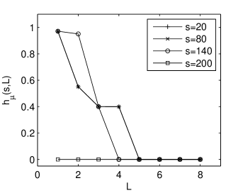
Figure 2: The entropy densities $h_{\mu}(s,L)$ of the time series coarse-grained with scales $20$ (plus signs), $80$ (crosses), $140$ (circles), and $200$ (squares) when the fraction of corrupted data points is $0.1$. Each point is averaged over $50$ realizations. There exists a convergence range of $L$ in $[5,8]$.

When there is no corrupted data, i.e. $r=0$, for $L\leq 3$ the global minima of $h_{\mu}(s,L)$ turn out to be $0$ for the multiples of $s=25=p/2$. As $L$ increases there appears the additional global minima for the other values of $s$. Finally the entropy densities $h_{\mu}(s,L)$ for the multiples of $s=5$ become the global minima when $L=5$ and even when $L>5$. This implies that $L\geq 5$ is the convergence range of $L$ as shown in Fig. 2. One can criticize that for the case of $s=1$, where the binary time series becomes $F=0^{25}1^{25}0^{25}1^{25}\cdots$, the pattern $0^{25}1^{25}$ can be completely revealed by taking $L$ larger than $50$. But it is contradictory to the first criterion in Eq. (6) when given the finite time series. Instead of taking $L$ as large as possible, we can get more relevant results by tuning the scale $s$ even for the small values of $L$ guaranteeing the significance of analysis.

If the corruption is taken into account, i.e. in cases of $r=0.1$ and $0.5$, the local minima for the odd multiples of $s=p/2$ become distinctive among other minima (Fig. 1 (b) and (c)). Moreover, the values of distinctive local minima in the landscape of $h_{\mu}(s,L)$ turn out to be independent of $L$ so that the structure scales $s^{*}$ are successfully determined and hence it is not necessary to specify the convergence range of $L$ as well as $L^{*}$.

Then why do the entropy densities for the odd multiples of $s=p/2$ remain minimized? The corruption definitely destroys the periodicity of time series and increases the randomness, therefore the overall values of local minima of $h_{\mu}(s,L)$ get larger than those for the case of $r=0$. However, the effect of corruption is not uniform. At first, without corruption $Y(sn)$ in Eq. (5) for the odd multiples of $s=p/2$ take the extreme values of $Y(t)$, precisely $Y(pn/2)=1$ for $n$ even and $Y(pn/2)=0$ for $n$ odd. Therefore the flip probability, defined as the probability that the sign of argument $Y(sn+s)-Y(sn)$ in Eq. (5) is flipped due to the corruption, is the least among for the other values of $s$. For example, if $Y(pn/2)$ remains unchanged as either $0$ or $1$ while $Y(pn/2+p/2)$ is replaced by a random number in $[0,1]$, the flip probability is $0$. On the other hand, for the case of $s=p$, if $Y(pn)$ remains unchanged as $1$ while $Y(pn+p)$ is replaced by a random number in $[0,1]$, the flip probability is $1$. As a result one can expect that when the periodic function is corrupted by noise, the most robust scale is not the period $p$ and its multiples but $p/2$ and its odd multiples. Based on this argument one can say that the existence of more than one distinctive local minimum naturally comes from the repetitive structure of the original function $Y(t)$, and that the patterns can appear in the different scales simultaneously.

For more general application to a continuous time series we can take the finer scales to increase the precision of measuring the structure scale. To show an efficient way to fine-tune $s$ we consider a corrupted periodic function with non-integer period, for example, for a continuous time $t$,

$$Y(t)=\left\{\begin{array}[]{ll}\cos^{2}\left(\frac{\pi}{77.6}t\right)&\quad\textrm{with probability}\,0.9\\ \eta&\quad\textrm{with probability}\,0.1\end{array}\right..$$ (8)

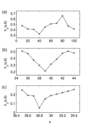
Figure 3: The entropy densities $h_{\mu}(s,L=6)$ measured in the precision of $10$ (a), $1$ (b), and $0.1$ (c), respectively.

To measure the structure scales (the odd multiples of $s=p/2$ for the case of discrete periodic functions), $s$ should be smaller than $0.1$. Instead of scanning the whole range of $s$, such as from $0.1$ to $100.0$, by the increment of $0.1$ we tune $s$ in a larger scale first and then move down to the smaller scales. The value of $L$ is set to $6$ according to the MEDM. Figure 3(a) shows the entropy densities for various $s$ in the order of $10$. The minimum of the entropy density occurs at $s=40$. We narrow the variation of $s$ down to $1$ around $40$. Then the minimum of the entropy density occurs at $s=39$ in Fig. 3(b) and we repeat the same process again. Finally, in Fig. 3(c) we obtain $s^{*}=38.8$ minimizing the entropy density, which is exactly a half period ($p/2$).

Finally, the MEDM can be applied to a periodic function with varying period by dividing the given time series into several regions and applying MEDM to each of them. Here we consider a periodic function with linearly decreasing period: for a continuous time $t$,

$$Y(t) = \left\{\begin{array}[]{ll}\cos^{2}\left(\frac{\pi}{p(t)}t\right)&\quad\textrm{with probability}\,0.9\\ \eta&\quad\textrm{with probability}\,0.1\end{array}\right.,$$ (11)

$$p(t) = p_{1}+\frac{p_{2}-p_{1}}{S}t,$$ (12)

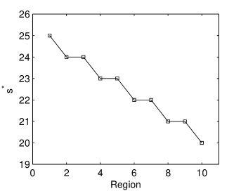
Figure 4: The temporal behavior of the structure scale $s^{*}$, where each point represents the $s^{*}$ for each partitioned region.

where the period continuously decreases from $p_{1}$ to $p_{2}$. We set $p_{1}$ to $50$, $p_{2}$ to $40$, and $S$ to $10^{5}$, respectively. The total time series is divided into $10$ regions and the MEDM is applied to each of them. For all the regions we tune $s$ in an order of $1$ and set $L$ to $6$ after testing in a way we described before. Figure 4 shows that the smallest structure scale $s^{*}$ decreases from $25=p_{1}/2$ in the first region to $20=p_{2}/2$ in the last one. These $s^{*}$s are exactly the half periods of the starting and ending parts of the original function. If we divide the time series into more regions and use the finer scales, then the resultant temporal behavior of structure scale gets closer to $p(t)/2$, where $p(t)$ is defined in Eq. (12), than before.

III Empirical data analysis

Now we apply the MEDM to analyze the financial time series of the S&P500 index from year 1983 to 2006. We used the tick-by-tick data. It is reasonable to think that the structure scale of S&P500 index for $24$ years would change from time to time. Hence the formalism of the last example in the previous Section is used. It should be noted that although the time series of the S&P500 index is not periodic, we can always measure the structure scale using MEDM whenever the series has patterns.

The total time span of the index data from February 1983 to April 2006 is divided into $279$ regions, i.e. each region for each month. For each region the structure scale is obtained then the temporal behavior of it will be analyzed. The unit of coarse-graining scale $s$ is set to $1$ tick, the finest resolution of the empirical S&P500 index data. On average there are $4$ ticks in one minute though the real time intervals between adjacent ticks are not equally distributed. One reasonable way to fix this problem is to obtain the structure scale $s^{*}_{tick}$ in a unit of tick for each month and multiply it by the average real time interval $\bar{\tau}_{tick}$ between ticks within that month. The resulting value $s^{*}=s^{*}_{tick}\cdot\bar{\tau}_{tick}$ will be the structure scale in a unit of time for each month.

Then we follow the four main steps of the MEDM to measure the structure scale of tick every month. For the first step the range of $s_{tick}$ is set to $1$ tick to $30$ ticks. The tick series with $s_{tick}=30$ has less than $900$ data points each month. By Eq. (6) the upper bound of $L$ is $9$. Considering the second criterion of choosing $L$, we set $L^{*}$ to $5$ by finding the convergence region of $L$ for the whole range of $s_{tick}$. Figure 5 shows the landscapes of entropy densities $h_{\mu}(s_{tick},L)$ only for the regions of February 1983 and April 2006. For the third step the structure scale $s^{*}_{tick}$ minimizing $h_{\mu}(s_{tick},5)$ is determined for each month. Three examples are shown in Fig. 6, where $h_{\mu}(s_{tick},5)$ is minimized at $s_{tick}=8$ for January 1987, at $s_{tick}=6$ for January 1996, and at $s_{tick}=2$ for January 2001, respectively. Unlike the case with the periodic time series, for each region there is only one structure scale over the range of $s$. After finding all the $s^{*}_{tick}$ we convert them into the real time scales by multiplying the average time interval between ticks for each month. Finally we get the temporal behavior of the structure length $s^{*}$ as shown in Fig. 7. During 1980’s and 1990’s $s^{*}$ decreases slowly but declines fast after late 1990’s.

We analyze the meaning of this result by considering the time scale by which the information flows among interacting agents in the stock market. The stock market price changes only when the agents in the stock market buy or sell. Since the agents make decisions based on the information they get, the information delivery time can be one of the most important factors for the changing rate of price. The information delivery time (IDT), defined as the time taken for the delivery of information from sources to agents, is assumed to be proportional to the average price change cycle. If the entropy density of the time series is measured with scale $s$ smaller than the IDT, it would be relatively high because the coarse-grained time series looks more random due to the high frequency noise. On the other hand, if $s$ is larger than IDT, we overlook the pattern embedded in the time series so fail to detect the structure scale and the coarse-grained time series looks more random too. Therefore, if the optimally closest scale to the IDT is used to detect the patterns in the time series, the entropy density for that scale would be minimized due to the repetitive structure of the price change. Consequently,

$$IDT\approx s^{*}.$$ (13)

The long-term decrease of $s^{*}$ from year 1986 to 2006 in Fig. 7 can be interpreted as the decrease of the information delivery time. The value of $s^{*}$ suddenly jumps down around year 1997, when the Internet was starting to spread widely, the fraction of online traders increased exponentially. These influenced the IDT of the stock market to become much shorter.

Since there does not exist any standardized way to measure the information delivery time, we suggest $s^{*}$ as one of candidates to measure it. IDT can be also used to measure the efficiency of the stock market: if the market is idealized with efficient market hypothesis (EMH) Mantegna2000 , then IDT will become $0$. In addition from our quantitative analysis IDT of the S&P500 index is about $17$ seconds in year 2006.

IV Conclusions

In this paper we have developed the minimum entropy density method (MEDM) to detect the structure scale of a given time series. This method is based on the assumption that the pattern in the time series is revealed most when the time series is coarse-grained with the structure scale defined as the scale minimizing the entropy density. We also showed that the MEDM is useful to detect the repetitive structures in the various time series if they have certain patterns.

Additionally, by applying the MEDM to the financial time series of S&P500 index we identified that the time scale with the most patterns showing, has decreased for the last twenty years. In other words the information flows faster than before. The MEDM has also been applied to Korea Composite Stock Price Index (KOSPI) from April 1992 to June 2003 with $1$ minute time interval Lee2006 . The structure scale of the KOSPI index, which can be interpreted as the IDT, had also decreased for ten years similar to S&P500 index. We believe this effect is real, considering that the Internet trading has become popular recently, which we think is one of the main factors of decreasing the IDT, in both U.S. and Korean stock market. Also, Yang and colleagues Yang2006 used the microscopic spin model to investigate the financial market and identified that the change of log-return distributions of financial stock markets can result from the increasing velocity of information flow, which implies that the IDT becomes shorter than before. Since IDT measures the efficiency of the stock market, by quantitative analysis we conclude that the efficiency of the U.S. stock market dynamics became close to EMH.

Figure 1: (Color online) The landscapes of entropy densities $h_{\mu}(s,L)$ of the periodic time series as functions of scale $s$ with block size $L=2$ (black circles), $4$ (red crosses), and $6$ (blue plus signs), respectively. The fraction of corrupted data points $r$ is $0$ (a), $0.1$ (b), and $0.5$ (c), respectively. For (b) and (c) each point is averaged over $50$ realizations and for a clear view we plotted $s$ to $100$ not to $s_{max}=200$.

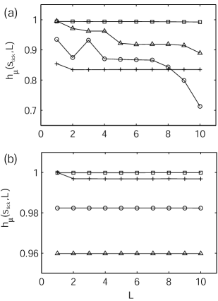
Figure 5: The entropy densities $h_{\mu}(s,L)$ of S&P500 index in February 1983 (a) and in April 2006 (b) using the time series with scale $s_{tick}=1$ (squares), $2$ (triangles), $5$ (circles), and $10$ (plus signs), respectively.

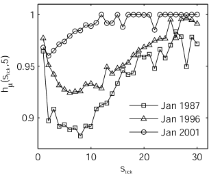
Figure 6: The entropy densities $h_{\mu}(s,L=5)$ of S&P500 index measured in January 1987 (squares), January 1996 (triangles), and January 2001 (circles), respectively.

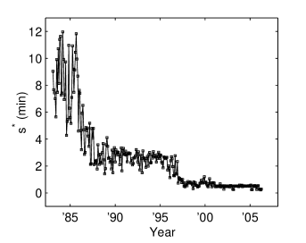
Figure 7: The temporal behavior of the structure scale $s^{*}$ of the S&P500 index measured monthly in a unit of time.

References

- (1) W. B. Arthur, S. N. Durlauf, and D. A. Lane, The Economy as an Evolving Complex System II (Perseus Books, 1997).
- (2) R. N. Mantegna and H. E. Stanley, An Introduction to Econophysics: Correlations and Complexity in Finance (Cambridge University Press, 2000).
- (3) J.-P. Bouchaud and M. Potters, Theory of Financial Risks (Cambridge University Press, 2000).
- (4) B. B. Mandelbrot, Quant. Finance 1, 124 (2001).
- (5) L. Kullmann, J. Kertész, and R. N. Mantegna, Physica A 287, 412 (2000).
- (6) L. Giada and M. Marsili, Physica A 315, 650 (2002).
- (7) E. E. Peters, Chaos and order in the capital markets (Wiely, 1991).
- (8) C.-K. Peng, S. V. Buldyrev, S. Havlin, M. Simons, H. E. Stanley, and A. L. Goldberger, Phys. Rev. E 49, 1685 (1994).
- (9) Y. Liu, P. Gopikrishnan, P. Cizeau, M. Meyer, C.-K. Peng, and H. E. Stanley, Phys. Rev. E 60, 1390 (1999).
- (10) D. Feldman, A Brief Introduction to Information Theory, Excess Entropy and Computational Mechanics, http://hornacek.coa.edu/dave/Tutorial/index.html (April 1998).
- (11) R. W. Clarke, M. P. Freeman, and N. W. Watkins, Phys. Rev. E 67, 016203 (2003).
- (12) C. R. Shalizi and K. L. Shalizi, preprint: cs.LG/0406011; in Proceedings of the 20th Annual Conference on Uncertainty in Artificial Intelligence (UAI-04), edited by M. Chickering and J. Halpern (AUAI Press, Virginia, 2004), pp. 504-511.
- (13) K. Marton and P. C. Shields, Annal. Prob. 22, 960 (1994); 24, 541 (1996).
- (14) J. W. Lee, J. B. Park, H.-H. Jo, J.-S. Yang, and H.-T. Moon, in Proceedings of the 9th Joint Conference on Information Sciences, Paper No. CIEF-231 (in press).
- (15) J.-S. Yang, S. Chae, W.-S. Jung, and H.-T. Moon, Physica A 363, 377 (2006).