Entropic elasticity of DNA with a permanent kink

Abstract

Many proteins interact with and deform double-stranded DNA in cells. Single-molecule experiments have studied the elasticity of DNA with helix-deforming proteins, including proteins that bend DNA. These experiments increase the need for theories of DNA elasticity which include helix-deforming proteins. Previous theoretical work on bent DNA has examined a long DNA molecule with many nonspecifically binding proteins. However, recent experiments used relatively short DNA molecules with a single, well-defined bend site. Here we develop a simple, theoretical description of the effect of a single bend. We then include the description of the bend in the finite worm like chain model (FWLC) of short DNA molecules attached to beads. We predict how the DNA force-extension relation changes due to formation of a single permanent kink, at all values of the applied stretching force. Our predictions show that high-resolution single-molecule experiments could determine the bend angle induced upon protein binding.

Keywords: DNA elasticity, force-extension measurements, helix-deforming proteins, transcription factors, bent DNA, theory.

1 Introduction

In cells, many different interactions between DNA and proteins occur, processes which are essential to gene expression, genome replication, and cellular DNA management. One major class of proteins interacts with DNA and mechanically deforms the double helix by wrapping, looping, twisting, or bending DNA (1, 2). Examples include DNA-packaging proteins and transcription factors which regulate gene expression. The mechanical deformation of the DNA may be important for gene expression: it has been suggested that DNA deformation by transcription factors may help other proteins bind to the DNA and initiate transcription.

The deformation of DNA by proteins can be detected in single-molecule force microscopy. In this experimental method, force is applied to individual DNA molecules and the DNA end-to-end extension is measured (figure 1). Single-molecule force microscopy has been used to detect the deformation of DNA caused by protein binding (3, 4, 5, 6, 7, 8). In these experiments the DNA end-to-end extension changes when a deformation-inducing protein binds. Varying the applied force allows one to probe the deformation and better understand the details of the protein-DNA interaction.

In this paper we focus on proteins that bend the DNA backbone and develop theoretical predictions of the force-extension behavior of bent DNA. Our description is based on the worm-like chain theory (WLC) (9, 10, 11). The WLC predicts the average end-to-end extension $z$ of a semiflexible polymer, given the force $F$ applied to the ends of the chain and the values of two constant parameters (the contour length $L$ and the persistence length $A$). However, DNA elastic behavior is altered by backbone-deforming proteins, an effect that is not included in the traditional WLC. Extended theories have been developed which combine the WLC treatment of DNA elasticity with local bends. Rivetti et al. addressed the case of zero applied force (12), while Yan and Marko have described the changes in the force-extension behavior of a long polymer to which many kink-inducing proteins can bind nonspecifically (13). Similarly, Popov and Tkachenko studied the effects of a large number of reversible kinks (14), Metzler et al. studied loops formed by slip-rings (15) , and Kulić et al. studied the high-force limit of a kinked polymer (16).

Previous theoretical work has focused on large numbers of reversible kinks or the limit of low or high applied force. However, recent single-molecule experiments have examined relatively short DNA molecules with a single specific kink site, over a range of applied force (7). Therefore a theory is needed which applies to (i) one kink site and (ii) a polymer of finite contour length ($L/A\sim 1-10$). Recently, we introduced a modified solution of the WLC applicable to polymers of this length, and demonstrated that applying the traditional WLC solution to molecules with $L/A\sim 1-10$ can lead to significant errors (17). Our finite worm-like chain solution (FWLC) includes both finite-length effects, often neglected in WLC calculations, and the effect of the rotational fluctuations of a bead attached to the end of the chain.

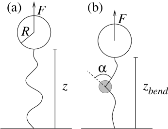
Figure 1: Typical experimental geometry of single-molecule force microscopy measurements. The DNA molecule is attached at one end to a surface and at the other end to a bead (radius $R$). A force $F$ is applied to the bead. (a) DNA molecule in the absence of bound protein. The mean end-to-end extension is $z$. (b) DNA molecule with a single bend-inducing protein bound. The protein bends the DNA backbone through the external angle $\alpha$ at the bend site. As a result, the mean extension decreases to $z_{bend}$.

Here we formulate a theoretical description of a single kink induced by a protein, and extend the FWLC treatment to include such local distortions. Our theory has a simple analytical formulation for the case of a force-independent bend angle, i.e., a rigid protein-DNA complex. Our predictions are relevant to experiments like those of Dixit et al. (7), which detect with high resolution a single bend induced in a relatively short DNA molecule. Although we will primarily focus on the case of a single bend angle, our method can also describe a kink which takes on different angles with different probabilities. This model could be relevant to a binding protein that can fluctuate between different binding conformations with different kink angles (18).

2 Theory

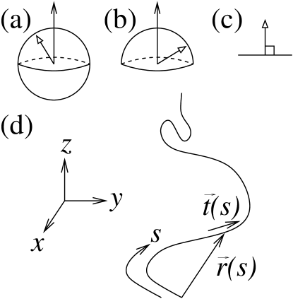
Figure 2: Boundary conditions and coordinates. (a) Unconstrained. (b) Half-constrained. (c) Normal. (d) Coordinates.

2.1 FWLC theory of unkinked DNA

The classic WLC model (10) and the FWLC theory (17), which includes finite-length effects, describe an inextensible polymer with isotropic bending rigidity. The bending rigidity is characterized by the persistence length, $A$, the length scale over which thermal fluctuations randomize the chain orientation. We assume that the twist is unconstrained and can be neglected (as is the case, for example, in optical tweezer experiments).

The chain energy function includes terms which represent the bending energy and the work done by the applied force:

$$E=\int_{0}^{\ell}ds\left(\frac{\kappa^{2}}{2}-f{\bf\hat{\bf z}}\cdot{\bf\hat{t}}\right),$$ (1)

where $E$ is the energy divided by the thermal energy $k_{B}T$, $\ell=L/A$, $s$ denotes arc length divided by the persistence length $A$, and all other lengths are similarly measured in units of $A$. The quantity $f$ is the force multiplied by $A/k_{B}T$, and we assume the force is applied in the $\hat{\bf z}$ direction. The total extension of the chain is $z=\int ds\ {\bf\hat{\bf z}}\cdot{\bf\hat{t}}$. The curvature $\kappa$ can be defined in terms of arc-length derivatives of the chain coordinate (figure 2d). If the chain conformation is described by a space curve ${\bf r}(s)$ and the unit vector tangent to the chain is ${\bf\hat{t}}(s)$, then $\kappa=\left|\frac{\partial^{2}{\bf r}}{\partial s^{2}}\right|=\left|\frac{\partial{\bf\hat{t}}}{\partial s}\right|$.

The chain partition function weights contributions from different polymer conformations (19, 20). If the ends of the chain are held at fixed orientations, we have

$$Z({\bf\hat{t}}_{f},\ell;{\bf\hat{t}}_{i},0)=\int D{\bf\hat{t}}\ \exp\left[-\int_{0}^{\ell}ds\left(\frac{1}{2}(\partial_{s}{\bf\hat{t}})^{2}-f{\bf\hat{\bf z}}\cdot{\bf\hat{t}}\right)\right],$$ (2)

where the integral in $D{\bf\hat{t}}$ is over all possible paths between the two endpoints of the chain with the specified orientations. The partition function can be interpreted as a propagator which connects the probability distribution for the tangent vector at point $s$, $\psi({\bf\hat{t}},s)$ to the same probability distribution at point $s^{\prime}$:

$$\psi({\bf\hat{t}},s)=\int d{\bf\hat{t}}^{\prime}\ Z({\bf\hat{t}},s;{\bf\hat{t}}^{\prime},s^{\prime})\ \psi({\bf\hat{t}}^{\prime},s^{\prime}).$$ (3)

From this relation, one can derive a Schrödinger-like equation, which describes the $s$ evolution of $\psi$ (10):

$$\frac{\partial\psi}{\partial s}=\left(\frac{\nabla^{2}}{2}+f\cos\theta\right)\psi.$$ (4)

Here $\nabla^{2}$ is the two-dimensional Laplacian on the surface of the unit sphere and $\cos\theta=\hat{\bf z}\cdot\hat{\bf t}$.

For relatively short DNA molecules ($\ell\sim 1-10$), the boundary conditions at the ends of the chain (17, 21) and bead rotational fluctuations become important. The boundary conditions are specified by two probability density functions, $\psi({\bf\hat{t}},s=0)$ and $\psi({\bf\hat{t}},s=L)$. The boundary conditions modify the force-extension relation, and enter the full partition function matrix element via

$$Z_{tot}=\int d{\bf\hat{t}}_{i}\ d{\bf\hat{t}}_{f}\ \psi({\bf\hat{t}}_{i},0)Z({\bf\hat{t}}_{i},0;{\bf\hat{t}}_{f},L)\psi({\bf\hat{t}}_{f},L).$$ (5)

Rotational fluctuations of the bead(s) attached to the end of the DNA complicate the analysis of experiments. What is observed and controlled is not the endpoint of the (invisible) DNA chain, but rather the bead’s center. The relation between these distinct points fluctuates as the bead performs rotational Brownian motion. The FLWC theory accounts for these fluctuations via an effective boundary condition at the end(s) of the chain, which depends on applied force, bead radius, and the nature of the link joining the bead to the polymer (17). We will study boundary conditions that are azimuthally symmetric; thus our end boundary conditions will be functions of $\hat{\bf t}\cdot\hat{\bf z}$ only.

2.2 Fixed-angle bend

We now suppose that our chain contains a permanent bend, whose location along the DNA, and angle, are fixed, independent of applied force. In this paper we will also neglect force-induced unbinding of the deforming protein. (These effects are straightforward to incorporate into our analysis.) In addition, we neglect twist stiffness, which is legitimate since we wish to study a single bend in a polymer with unconstrained twist. (Twist stiffness effects will be important for experiments in which multiple bends occur or twist is constrained.)

The Schrödinger-like equation (4) must be modified by the inclusion of a “bend operator” which transforms $\psi$ at the bend. Suppose that the kink occurs at position $s_{o}$. Given the tangent-vector probability distribution $\psi$ at $s_{o}-\epsilon$ (where $\epsilon$ is infinitesimal), our goal is to determine $\psi({\bf\hat{t}},s_{o}+\epsilon)$, the distribution just after the kink. If we denote the exterior angle of the kink by $\alpha$, then ${\bf\hat{t}}_{s_{o}-\epsilon}\cdot{\bf\hat{t}}_{s_{o}+\epsilon}=\cos\alpha$. Because twist is unconstrained, we may average over rotations; effectively, the bend occurs with uniform probability in the azimuthal angle: if ${\bf\hat{t}}_{s_{o}-\epsilon}$ points directly along the $\hat{\bf z}$-axis, then ${\bf\hat{t}}_{s_{o}+\epsilon}$ is uniformly distributed in a cone at angle $\alpha$ to the $\hat{\bf z}$-axis.

The bend operator then can be written using the kernel

$$K_{\alpha}({\bf\hat{t}},{\bf\hat{t}}^{\prime})=\frac{1}{2\pi}\delta({\bf\hat{t}}\cdot{\bf\hat{t}}^{\prime}-\cos\alpha).$$ (6)

The probability distribution $\psi({\bf\hat{t}}^{\prime},s_{o}-\epsilon)$ of tangent-vector angles just before the kink is related to the distribution $\psi({\bf\hat{t}},s_{o}+\epsilon)$ just after the kink by

$$\psi({\bf\hat{t}},s_{o}+\epsilon)=\int d{\bf\hat{t}}^{\prime}\ K_{\alpha}({\bf\hat{t}},{\bf\hat{t}}^{\prime})\ \psi({\bf\hat{t}}^{\prime},s_{o}-\epsilon).$$ (7)

Below (section 3.2) we show that spherical harmonics diagonalize the operator (6).

2.2.1 Distribution of bend angles

Suppose that the bend occurs not for a single fixed angle, but a distribution of angles. We assume that ${\bf\hat{t}}_{s_{o}-\epsilon}\cdot{\bf\hat{t}}_{s_{o}+\epsilon}=\cos\alpha=u$ is distributed according to the probability density function $h(u)$, where $h$ is normalized so that $\int d\phi\int du\ h(u)=1$. Then the bend-operator kernel can be written as an integral over the probability distribution:

$$K_{h}({\bf\hat{t}},{\bf\hat{t}}^{\prime})=\frac{1}{2\pi}\int_{-1}^{1}du\ h(u)\ \delta({\bf\hat{t}}\cdot{\bf\hat{t}}^{\prime}-u).$$ (8)

3 Calculation

The main quantity of interest in single-molecule experiments is the force-extension relation, which can be determined by solving equation (4) for the tangent-vector probability distribution $\psi({\bf\hat{t}},s)$. The Schrödinger-like equation is solved using separation of variables in $s$ and ${\bf\hat{t}}$, where the angular dependence is expanded in spherical harmonics (10).

$$\psi({\bf\hat{t}},s)=\sum_{j=0}^{\infty}\Psi_{j}(s)Y_{j0}({\bf\hat{t}}).$$ (9)

(By azimuthal symmetry, only the $m=0$ terms will enter in our formulae.) In the basis of spherical harmonics, the operator in equation (4) is a symmetric tridiagonal matrix $H$ with diagonal terms

$$H_{j,j}=-\frac{j(j+1)}{2},$$ (10)

and off-diagonal terms

$$H_{j,j+1}=\frac{f(j+1)}{\sqrt{(2j+1)(2j+3)}}.$$ (11)

The vector of coefficients at $s$ is ${\bf\Psi}(s)=e^{sH}{\bf\Psi}(0)$ (10, 17). This expression for $\psi({\bf\hat{t}},s)$ is exact if the infinite series of spherical harmonics is used.

3.1 Force-extension relation

Given the boundary conditions ${\bf\Psi}(s=0)$ and ${\bf\Psi}(s=\ell)$, the partition function is

$$Z = {\bf\Psi}^{T}(s=\ell)e^{\ell H}{\bf\Psi}(s=0),$$ (12)

$$= \sum_{j,k}\Psi_{j}(s=\ell)[e^{\ell H}]_{jk}\Psi_{k}(s=0).$$ (13)

The fractional extension of the chain is

$$\frac{z}{L}=\frac{1}{\ell}\frac{\partial\ln Z}{\partial f}.$$ (14)

We work in the ensemble relevant to most experiments, where the extension is determined for fixed applied force (different ensembles are not equivalent for single finite-length molecules (22, 23, 24)). Equation (14) applies for a chain of any length. However, we can show the structure of the partition function more clearly by separating $\ln Z$ into two terms: one representing an infinite chain and a finite-length correction (17). Let $B=e^{H}$, denote by $\lambda_{*}$ the largest eigenvalue of $B$, and let ${\cal B}=B/\lambda_{*}$. Then ${\cal B}$ has eigenvalues with magnitude less than or equal to 1 and the logarithm of the partition function can be written

$$\ln Z=\ell\ln\lambda_{*}+\ln[{\bf\Psi}^{T}(s=\ell){\cal B}^{\ell}{\bf\Psi}(s=0)].$$ (15)

Only the first term is considered in the usual WLC solution; the second term is the finite-length correction (17). Equation (15) is an exact expression for $\ln Z$ which is difficult to evaluatae analytically. We numerically calculate the force-extension relation by using equation (15) with the series truncated after $N$ terms. This expression can be accurately numerically calculated, and the truncation error determined by comparing the results with different $N$. Our calculations use $N=30$ unless otherwise specified.

3.1.1 Boundary conditions and bead rotational fluctuations

The boundary conditions at $s=0$ and $s=\ell$ affect the force-extension relation, because they alter the partition function as shown in equation (15). Some experiments appear to implement “half-constrained” boundary conditions, where the polymer is attached to a planar wall by a freely rotating attachment point, and the wall is perpendicular to the direction of applied force (25). In this case the tangent vector at the end of the chain can point in any direction on the hemisphere outside the impenetrable surface (figure 2(b)). The effects of different boundary conditions on the force-extension relation are considered in detail in reference (17). In the “unconstrained” boundary condition the tangent vector at the end of the chain is free to point in any direction on the sphere (in $4\pi$ of solid angle, figure 2a). In this case $\psi(\hat{\bf t})$ is independent of $\cos\theta$ and ${\bf\Psi}=(1,0,\cdots,0)$. In the “half-constrained” boundary conditions (figure 2b), the tangent vector at the end of the chain can point in any direction on the hemisphere outside the impenetrable surface; then the leading coefficients of ${\bf\Psi}$ are 1, 0.8660, 0, -0.3307, 0, 0.2073, 0. In the “normal” boundary condition, the tangent vector at the end of the chain is parallel to the $\hat{\bf z}$ axis, normal to the surface (figure 2c). Then the coefficients of ${\bf\Psi}$ are all equal to 1 (26).

The FWLC formulation can also average over rotational fluctuations of spherical bead(s) attached to one or both ends of the polymer chain. The result is an effective boundary condition that depends on applied force and bead radius (17). Both the case of perpendicular wall attachment and bead attachment generate boundary conditions that are invariant under rotations about the $\hat{z}$ axis (the direction in which force is applied), and hence give boundary states of the form given in equation (9).

3.2 Bend operator

We wish to represent the bend operator (equation (7)) in terms of spherical harmonics; the operator is diagonal in this basis. Denote $x={\bf\hat{t}}\cdot{\bf\hat{t}}^{\prime}$ and note that any function of $x$ with $-1\leq x\leq 1$ can be written as a series of Legendre polynomials (27):

$$K_{\alpha}(x)=\sum_{l=0}^{\infty}k_{l}P_{l}(x).$$ (16)

The $k_{l}$ are determined by projecting the kernel $K$ onto the Legendre polynomials, using the normalization relation $\int_{-1}^{1}P_{l^{\prime}}(x)P_{l}(x)dx=\frac{2}{2l+1}\delta_{ll^{\prime}}$. Therefore

$$k_{l} = \frac{2l+1}{4\pi}\int_{-1}^{1}\delta(x-\cos\alpha)P_{l}(x)dx,$$ (17)

$$= \frac{2l+1}{4\pi}P_{l}(\cos\alpha).$$ (18)

Next we use the addition theorem for spherical harmonics (27)

$$P_{l}({\bf\hat{t}}\cdot{\bf\hat{t}}^{\prime})=\frac{4\pi}{2l+1}\sum_{m=-l}^{l}Y_{lm}^{*}(\hat{\bf t}^{\prime})Y_{lm}(\hat{\bf t}),$$ (19)

Substituting equations (19) and (18) in equation (16), we have

$$K_{\alpha}({\bf\hat{t}},{\bf\hat{t}}^{\prime})=\sum_{l=0}^{\infty}P_{l}(\cos\alpha)\sum_{m=-l}^{l}Y_{lm}^{*}(\hat{\bf t}^{\prime})Y_{lm}(\hat{\bf t}).$$ (20)

Note that if $\alpha=0$, the kink operator reduces to the identity because $P_{l}(1)=1$.

The probability distribution $\psi$ just before the bend is

$$\psi({\bf\hat{t}}^{\prime},s_{o}-\epsilon)=\sum_{j=0}^{\infty}\sum_{k=-j}^{j}\Psi_{jk}(s_{o}-\epsilon)Y_{jk}(\hat{\bf t}^{\prime}).$$ (21)

Note that in the case of azimuthal symmetry, the terms with $k\neq 0$ are zero. To determine $\psi$ just after the bend, we substitute the expressions in equations (20) and (21) into the formula

$$\psi({\bf\hat{t}},s_{o}+\epsilon)=\int d{\bf\hat{t}}^{\prime}\ K_{\alpha}({\bf\hat{t}},{\bf\hat{t}}^{\prime})\ \psi({\bf\hat{t}}^{\prime},s_{o}-\epsilon).$$ (22)

The expression simplifies by the orthonormality of spherical harmonics:

$$\psi({\bf\hat{t}},s_{o}+\epsilon) = \sum_{l=0}^{\infty}P_{l}(\cos\alpha)\sum_{m=-l}^{l}Y_{lm}(\hat{\bf t})\sum_{j=0}^{\infty}\sum_{k=-j}^{j}\Psi_{jk}(s_{o}-\epsilon)\int d{\bf\hat{t}}^{\prime}\ Y_{lm}^{*}(\hat{\bf t}^{\prime})Y_{jk}(\hat{\bf t}^{\prime})$$ (23)

$$= \sum_{l=0}^{\infty}P_{l}(\cos\alpha)\sum_{m=-l}^{l}Y_{lm}(\hat{\bf t})\sum_{j=0}^{\infty}\sum_{k=-j}^{j}\Psi_{jk}(s_{o}-\epsilon)\delta_{jl}\delta_{mk}$$ (24)

$$= \sum_{l=0}^{\infty}\sum_{m=-l}^{l}P_{l}(\cos\alpha)\Psi_{lm}(s_{o}-\epsilon)Y_{lm}(\hat{\bf t}).$$ (25)

The transformation can thus be written $\Psi_{lm}(s_{o}+\epsilon)=P_{l}(\cos\alpha)\Psi_{lm}(s_{o}-\epsilon)$. The probability distribution just after the kink differs from the distribution before the kink only in the multiplication of each term in the series by $P_{l}(\cos\alpha)$. We can represent the transformation by a diagonal matrix $W$ such that

$${\bf\Psi}(s_{o}+\epsilon)=W{\bf\Psi}(s_{o}-\epsilon).$$ (26)

Because $\psi$ is azimuthally symmetric (only the $m=0$ terms appear in the series expansion), $W$ has entries $W_{l,l}=P_{l-1}(\cos\alpha)$.

3.2.1 Distribution of bend angles

The representation of the bend operator in terms of spherical harmonics remains simple when the bend contains a distribution of angles described by $h(u)$ (equation (8)). As above, we expand $K_{h}(x)$ in Legendre polynomials, $K_{h}(x)=\sum k_{l}P_{l}(x).$ The $k_{l}$ are the projection of $h(x)$ onto Legendre polynomials:

$$k_{l}=\frac{2l+1}{4\pi}\int_{-1}^{1}dx\ h(x)P_{l}(x).$$ (27)

The calculation is then identical to the case of a single bend angle, with the result $\Psi_{lm}(s_{o}+\epsilon)=k_{l}\Psi_{lm}(s_{o}-\epsilon)$. We can represent the transformation by a diagonal matrix $W_{h}$ such that

$${\bf\Psi}(s_{o}+\epsilon)=W_{h}{\bf\Psi}(s_{o}-\epsilon).$$ (28)

3.3 Force-extension relation with bend

Once the matrix $W$ (which represents the bend operator in the basis of spherical harmonics) has been determined, calculation of the force-extension relation is straightforward. Suppose a single bend occurs at fractional position $a$ along the chain. The partition function with a bend is

$$Z_{b}={\bf\Psi}^{T}(s=\ell)e^{(1-a)\ell H}We^{a\ell H}{\bf\Psi}(s=0),\\$$ (29)

As before, we let $B=e^{H}$, denote by $\lambda_{*}$ the largest eigenvalue of $B$, and define ${\cal B}=B/\lambda_{*}$. Using $e^{\ell H}=\lambda_{*}^{\ell}{\cal B}^{\ell}$, the logarithm of the partition function is

$$\ln Z_{b}=\ell\ln\lambda_{*}+\ln[{\bf\Psi}^{T}(s=\ell)\ {\cal B}^{(1-a)\ell}W{\cal B}^{a\ell}\ {\bf\Psi}(s=0)].$$ (30)

As above, the extension is $z/L=\ell^{-1}\ \partial\ln Z/\partial f.$

4 Results

Here we predict the magnitude of extension change induced by a single bend, in order to understand when such single-bending events will be experimentally detectable. We describe how the extension change induced by a bend depends on applied force, bend angle, contour length, and the position of the bend.

In figure 3 we show the change in extension induced by a bend: the extension of the chain without the bend minus the extension of the chain with the bend. As expected, the extension change is larger when the bend angle is larger. In addition, we find that the change in extension has a maximum near an applied force of 0.1 pN. At this force, the change in extension due to the bend is a significant fraction of the persistence length (10-30 nm for $A=50$ nm).

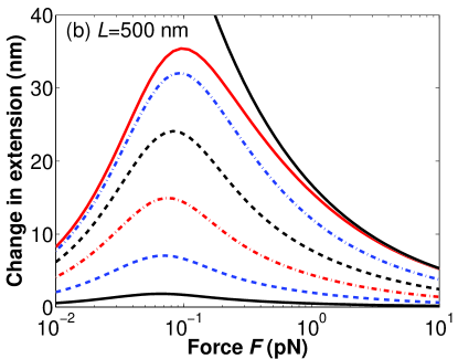
Figure 3: Change in extension due to a bend as a function of force, determined by subtracting the extension of the chain with the bend from the extension without the bend. The contour length is (A) $L$=200 nm and (B) $L$=500 nm. For larger contour lengths, the prediction is similar to (B). We assume $A=50$ nm, the bend is at the midpoint of the polymer, a bead of radius 250 nm is attached to one end of the chain, and half-constrained boundary conditions. For the largest bend angle, we show for comparison the prediction of Kulić et al. (16), which is valid in the high-force limit.

For the largest bend angle, we show for comparison the prediction of Kulić et al. (16). The Kulić et al. result is valid in the high-force limit, and we find that their prediction and our result converge as the force becomes large. The Kulić et al. result is valuable because it is a simple analytical expression. Although our results are obtained numerically, they are valid over the entire force range.

As the applied force increases, the polymer becomes more stretched and aligned with the force, decreasing the effect of the bend. For a classical elastic rod where thermal fluctuations are a weak perturbation the characteristic propagation length of elastic deformations is $\sqrt{k_{b}T\ A/F}$. Therefore, as the force increases, the region of the chain experiencing a significant deflection due to the bend drops. By this argument, one might expect that the largest change in extension due to the bend will occur for the lowest values of the applied force. However, as the force applied to the ends of the polymer goes to zero, the extension also approaches zero (on average, there will be no separation of the two ends). In this case the change in extension due to the bend approaches zero. The effect of the bend is therefore largest at intermediate force, where the molecule is extended by the force but not fully extended.

We predicted the change in extension due to the bend with and without a bead attached to one end of the DNA, and for different values of the bead radius. In all cases, we predict similar values for the change in extension due to a bend (not shown).

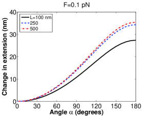
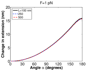
Figure 4: Change in extension due to a bend as a function of angle. (A) F=0.1 pN. (B) F=1 pN. We assume $A=50$ nm, the bend is at the midpoint of the polymer, a bead of radius 250 nm is attached to one end of the chain, and half-constrained boundary conditions.

In figure 4 we show how the change in extension induced by the bend varies with bend angle. The dependence of the extension change on angle is strong, suggesting that high-resolution experiments could measure the bend angle by measuring the change in extension due to a bend. For larger values of the applied force ($F\geq$1 pN), the result is independent of contour length of the polymer. However at low force ($F$=0.1 pN), where the change in extension due to a bend is largest, the results depend on the polymer contour length.

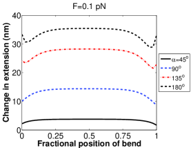
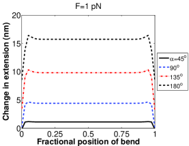
Figure 5: Change in extension due to a bend as a function of the position of the bend along the polymer. (A) F=0.1 pN. (B) F=1 pN. Note the difference in scale between the two panels. We assume $A=50$ nm, $L=$500 nm, a bead of radius 250 nm is attached to one end of the chain, and half-constrained boundary conditions.

The dependence on the position of the bend is weak, unless the bend is within a few percent of one end of the polymer (figure 5). We note that the curves in figure 5 are not reflection symmetric about the middle of the polymer. This occurs because we assume one end of the polymer ($s=0$) is attached to a fixed surface, while the other end of the polymer ($s=1$) is attached to a bead which can undergo rotational fluctuations. We chose to plot this case because it is a typical experimental geometry; in the case that both ends of the polymer experience identical boundary conditions, then the effects of a bend obey reflection symmetry about the middle of the polymer.

5 Discussion

We have described a theory of DNA elasticity applicable to bent DNA molecules. The finite worm-like chain model (FWLC) of polymer elasticity extends the WLC to polymers with $L/A\sim 1-10$ (17). The FWLC includes chain-end boundary conditions and rotational fluctuations of a bead attached to the end of the polymer, modifications which are important for polymers with contour length a few times the persistence length.

This work allows predictions of DNA force-extension behavior when a single bend occurs at a specified point along the chain. When the bend angle is constant (independent of applied force) the bend operator is diagonal in the basis of spherical harmonics, allowing straightforward calculation of the effects of a bend. This mathematical description of a bend is suitable both for a bend with a single angle and for bends with a distribution of different bend angles.

We demonstrate that the change in polymer end-to-end extension induced by the bend can be a significant fraction of the polymer persistence length: $\Delta z/A\sim 0.2-0.7$ for bend angles of 90-180^o, or $\Delta z\sim 10-35$ nm for dsDNA, which has persistence length of approximately 50 nm. The change in extension due to the bend is predicted to show a maximum for applied force around 0.1 pN; for larger force the polymer conformation becomes highly extended and the influence of the bend decreases, while for low force the polymer extension approaches zero, independent of the presence of the bend.

The alterations in polymer extension induced by the bend should be detectable in high-resolution single-molecule experiments. Since recent work in single-molecule optical trapping with DNA has demonstrated a resolution of a few nm(28, 29), DNA extension changes of 10-35 nm due to a bend should be detectable. Furthermore, the predicted change in extension strongly depends on the bend angle, suggesting that high-resolution single-molecule experiments could directly estimate the angle of a protein-induced bend.

References

- (1) Dickerson, R. E. Nucleic Acids Research 1998, 26, 1906-1926.
- (2) Luscombe, N.; Austin, S.; Berman, H.; Thornton, J. Genome Biology 2000, 1, 1.
- (3) van Noort, J.; Verbrugge, S.; Goosen, N.; Dekker, C.; Dame, R. T. Proceedings of the National Academy of Sciences of the United States of America 2004, 101, 6969-6974.
- (4) Skoko, D.; Wong, B.; Johnson, R. C.; Marko, J. F. Biochemistry 2004, 43, 13867-13874.
- (5) Yan, J.; Skoko, D.; Marko, J. F. Physical Review E 2004, 70, 011905.
- (6) van den Broek, B.; Noom, M. C.; Wuite, G. J. L. Nucleic Acids Research 2005, 33, 2676-2684.
- (7) Dixit, S.; Singh-Zocchi, M.; Hanne, J.; Zocchi, G. Physical Review Letters 2005, 94, 118101.
- (8) McCauley, M.; Hardwidge, P. R.; Maher, L. J.; Williams, M. C. Biophysical Journal 2005, 89, 353-364.
- (9) Bustamante, C.; Marko, J. F.; Siggia, E. D.; Smith, S. Science 1994, 265, 1599-1600.
- (10) Marko, J. F.; Siggia, E. D. Macromolecules 1995, 28, 8759-8770.
- (11) Bouchiat, C.; Wang, M. D.; Allemand, J. F.; Strick, T.; Block, S. M.; Croquette, V. Biophysical Journal 1999, 76, 409-413.
- (12) Rivetti, C.; Walker, C.; Bustamante, C. Journal of Molecular Biology 1998, 280, 41-59.
- (13) Yan, J.; Marko, J. F. Physical Review E 2003, 68, 011905.
- (14) Popov, Y. O.; Tkachenko, A. V. Physical Review E 2005, 71, 051905.
- (15) Metzler, R.; Kantor, Y.; Kardar, M. Phys. Rev. E 2002, 66, 022102.
- (16) Kulic, I. M.; Mohrbach, H.; Lobaskin, V.; Thaokar, R.; Schiessel, H. Physical Review E 2005, 72, 041905.
- (17) Li, J.; Nelson, P. C.; Betterton, M. D. “DNA entropic elasticity for short molecules attached to beads”, 2005 http://arxiv.org/abs/physics/0601185.
- (18) Parkhurst, L. J.; Parkhurst, K. M.; Powell, R.; Wu, J.; Williams, S. Biopolymers 2001, 61, 180-200.
- (19) Fixman, M.; Kovac, J. Journal of Chemical Physics 1973, 58, 1564-1568.
- (20) Yamakawa, H. Pure and Applied Chemistry 1976, 46, 135-141.
- (21) Samuel, J.; Sinha, S. Physical Review E 2002, 66, 050801.
- (22) Dhar, A.; Chaudhuri, D. Physical Review Letters 2002, 89, 065502.
- (23) Keller, D.; Swigon, D.; Bustamante, C. Biophysical Journal 2003, 84, 733-738.
- (24) Sinha, S.; Samuel, J. Physical Review E 2005, 71, 021104.
- (25) Nelson, P. C.; Brogioli, D.; Zurla, C.; Dunlap, D. D.; Finzi, L. “Quantitative analysis of tethered particle motion”, 2005 submitted.
- (26) Note that for the computation of the force-extension relation, it is not necessary to properly normalize the probability distribution, because we are computing the derivative of the logarithm of . Our expressions for the probability distribution vectors will neglect the constant normalization factor.
- (27) Jackson, J. D. Classical Electrodynamics; John Wiley and Sons: New York, second ed.; 1975.
- (28) Perkins, T. T.; Li, H. W.; Dalal, R. V.; Gelles, J.; Block, S. M. Biophysical Journal 2004, 86, 1640-1648.
- (29) Nugent-Glandorf, L.; Perkins, T. T. Optics Letters 2004, 29, 2611-2613.