Suppressing the Rayleigh-Taylor instability with a rotating magnetic field

Abstract

The Rayleigh-Taylor instability of a magnetic fluid superimposed on a non-magnetic liquid of lower density may be suppressed with the help of a spatially homogeneous magnetic field rotating in the plane of the undisturbed interface. Starting from the complete set of Navier-Stokes equations for both liquids a Floquet analysis is performed which consistently takes into account the viscosities of the fluids. Using experimentally relevant values of the parameters we suggest to use this stabilization mechanism to provide controlled initial conditions for an experimental investigation of the Rayleigh-Taylor instability.

I Introduction

The Rayleigh-Taylor instability Rayleigh , Taylor , Lewis is a classical hydrodynamic instability Chandrasekhar with relevance in such diverse fields as plasma physics, astrophysics, meteorology, geophysics, inertial confinement fusion and granular media, for a review see, e.g., Sharp . Generically this instability develops if a layer of liquid is superimposed to an immiscible and less dense liquid such that the potential energy of the system can be reduced by interchanging the liquids. Consequently, the initially plane interface between the liquids becomes unstable and the characteristic dimples and spikes develop resulting finally in a stable layering with the lighter fluid on top of the heavier one.

A quantitative experimental investigation of the Rayleigh-Taylor instability requires reliable control of the initial condition. Standard procedures like suddenly removed partitions between the fluids LiRe , Da or quickly turning the experimental cell upside down PlWh , Lange clearly produce unpredictable initial perturbations. It is much more convenient to use some additional mechanism which first stabilizes the unstable layering of the liquids and may later be switched off instantaneously. It is well known that the Rayleigh-Taylor instability may be suppressed, e.g., by vertical oscillation of the system Wolf1 , Wolf2 and by appropriate temperature gradients Burgess . The first mechanism is likely to induce uncontrolled initial surface deflections when stopped, in the second one it is difficult to abruptly switch off the stabilization.

In the present paper we investigate the possibility to stabilize a potentially Rayleigh-Taylor unstable system involving a magnetic fluid by external magnetic fields. We will show that for experimentally relevant parameter values moderate fields strengths which can easily be switched on and off are sufficient to achieve the desired stabilization.

Magnetic fluids are suspensions of ferromagnetic nano-particles in carrier liquids with the hydrodynamic properties of Newtonian fluids and the magnetic properties of super-paramagnets Rosensweig , Cowley . It is well known that a magnetic field parallel to the plane interface between a ferrofluid and a non-magnetic fluid suppresses interface deflections with wave vector in the direction of the field Rosensweig . This may be used to stabilize the Rayleigh-Taylor instability in two-dimensional situations where the interface is line, as e. g. in a Hele-Shaw cell. In the more natural three-dimensional setting we are interested in here a static magnetic field parallel to the undisturbed interface is not sufficient to stabilize the flat interface since perturbation with wave vectors perpendicular to the magnetic field will still grow as in the absence of the field. We therefore propose to use a spatially homogeneous magnetic field rotating in the plane of the undisturbed interface and determine appropriate values of the field amplitude and rotation frequency. An alternative possibility is to use a static inhomogeneous magnetic field with the magnetic force counterbalancing gravity Zelazo . This method was used in Carles to investigate the 2-d Rayleigh-Taylor instability in a Hele-Shaw cell.

Before embarking upon the detailed analysis we would like to mention three characteristic features of our method. Firstly, we will show that a rotating magnetic field is unable to suppress all possible unstable modes of the system. In fact it can only stabilize surface deflections with wavenumber modulus larger than some threshold value. Perturbations with very long wavelength are, however, not a serious problem in real experiments because these are suppressed automatically by the finite geometry of the sample. Secondly, it is well-known that in analogy with the Faraday instability an oscillating magnetic field will induce new instabilities at wave numbers which without field were stable FaSn , Mahr . In our analysis we keep track of these unstable modes and determine the magnetic field strength such that no new instabilities may occur. For suppressing these new modes viscous losses in the liquids will be decisive which is the reason why the viscosities of the two liquids will be consistently taken into account in the analysis. Finally, due to the dispersed magnetic grains ferrofluids have usually comparatively high densities. We therefore specialize to the case in which the upper, heavier layer is formed by the magnetic fluid. This should be the typical situation in experiments. Nevertheless a similar analysis with analogous results is possible for the reverse situation with the ferrofluid at the bottom of the system superimposed by an even denser non-magnetic liquid.

The paper is organized as follows. In section II we collect the basic equations and boundary conditions. In Section III we linearize these equations around the reference state of a plane interface between the liquids. Section IV contains the Floquet theory to determine the boundaries separating stable from unstable regions in the parameter plane. After shortly discussing two approximate treatments of the fluid viscosities in section V we present the results of our analysis in section VI. Finally section VII contains some discussion.

II Basic equations

We consider a ferrofluid with density $\rho^{(2)}$ superimposed on a non-magnetic fluid of lower density $\rho^{(1)}<\rho^{(2)}$, see Fig. 1. Both layers are assumed to be infinite in horizontal as well as in vertical direction. The densities and the respective viscosities $\eta^{(1)}$ and $\eta^{(2)}$ are taken to be constant. The liquids are immiscible and the interface between them is parametrized by $z=\zeta(x,y,t)$. We will study the stability of a flat interface which we take as the $x$-$y$-plane of our coordinate system, the undisturbed interface is hence given by $\zeta(x,y,t)\equiv 0$. In the absence of a magnetic field this situation is unstable due to the Rayleigh-Taylor instability Rayleigh ; Taylor ; Chandrasekhar .

In the presence of an external magnetic field ${\bf H}$ the magnetic fluid builds up a magnetization ${\bf M}$ which is assumed to be a linear function of the field, ${\bf M}=\chi{\bf H}$, where $\chi$ denotes the susceptibility related to the relative permeability by $\mu_{r}=1+\chi$. Both liquids are subject to the homogeneous gravitational field acting in negative $z$-direction and to the interface tension $\sigma$ acting at their common interface. The magnetic fluid is additionally influenced by the magnetic force density $({\bf M}\nabla){\bf H}$ resulting from the externally imposed spatially homogeneous magnetic field ${\bf H}_{0}=H_{0}(\cos(\Omega t),\sin(\Omega t),0)$ rotating with constant angular frequency $\Omega$ in the $x$-$y$-plane.

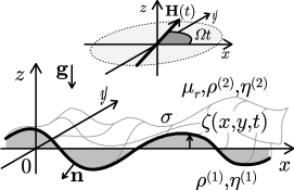
Figure 1: Sketch of the system under consideration. A ferrofluid of relative permeability $\mu_{r}$, density $\rho^{(2)}$ and viscosity $\eta^{(2)}$ is superimposed on a non-magnetic fluid with density $\rho^{(1)}<\rho^{(2)}$ and viscosity $\eta^{(1)}$. The normal vector ${\bf n}$ on the interface $\zeta(x,y,t)$ points into the non-magnetic liquid. The vector ${\bf g}$ denotes the gravitational acceleration, $\sigma$ is the interface tension. The system is subjected to a horizontal rotating magnetic field ${\bf H}_{0}=H_{0}(\cos(\Omega t),\sin(\Omega t),0)$ with angular frequency $\Omega$.

The time evolution of the system is governed by the following set of equations. The incompressibility of both liquids gives rise to the continuity equations for the velocity fields ${\bf v}^{(j)}$

$$\nabla\cdot{\bf v}^{(j)}=0\;,$$ (1)

with $j=1,2$ where here and in the following the lower (i.e. non-magnetic) fluid parameters are denoted with superscript $(1)$ and the higher (magnetic) one with superscript $(2)$. The hydrodynamic equations of motion are the Navier-Stokes equations

$$\rho^{(j)}\left(\partial_{t}+{\bf v}^{(j)}\cdot\nabla\right){\bf v}^{(j)}=\nabla\cdot T^{(j)}+\rho^{(j)}{\bf g}$$ (2)

with ${\bf g}=(0,0,-g)$ denoting the acceleration due to gravity and the stress tensors $T_{\ell m}^{(j)}$ given by

$$\begin{split}T_{\ell m}^{(j)}=&-\left(p^{(j)}+\frac{\mu_{0}}{2}H^{(j)2}\right)\delta_{\ell m}\\[4.30554pt] &+B_{\ell}^{(j)}H_{m}^{(j)}+\eta^{(j)}\left(\partial_{\ell}v_{m}^{(j)}+\partial_{m}v_{\ell}^{(j)}\right)\;.\end{split}$$ (3)

Here $p^{(j)}$ denotes the pressure in each liquid, and ${\bf B}^{(j)}=\mu_{0}({\bf H}^{(j)}+{\bf M}^{(j)})$ is the respective magnetic induction. Note that also the stress tensor for the non-magnetic liquid contains contributions from the magnetic field which, however, are divergence free and therefore do not give rise to a force density in the lower fluid.

For values of $\Omega$ relevant to the present investigation radiative effects are negligible and the magnetic field has to obey the magneto-static Maxwell equations

$$\begin{split}\nabla\cdot{\bf B}^{(j)}&=0\\[4.30554pt] \nabla\times{\bf H}^{(j)}&=0\end{split}\quad.$$ (4)

In view of the second equation it is convenient to introduce scalar magnetic potentials $\Phi^{(j)}$ according to ${\bf H}^{(j)}=-\nabla\Phi^{(j)}$. These potentials then fulfill the Laplace equations

$$\nabla^{2}\Phi^{(j)}=0\;.$$ (5)

The above equation have to be supplemented by appropriate boundary conditions. Far from the interface the velocities must remain bounded,

$$\lim_{z\rightarrow\pm\infty}|{\bf v}^{(j)}|<\infty\;,$$ (6)

and the magnetic field must be equal to the externally imposed field,

$$\lim_{z\rightarrow\pm\infty}-\nabla\Phi^{(j)}={\bf H}_{0}\;.$$ (7)

To formulate the boundary conditions at the interface $z=\zeta(x,y,t)$ we define the normal vector ${\bf n}$ by

$${\bf n}=-\frac{\nabla(z-\zeta(x,z,t))}{\left|\nabla(z-\zeta(x,z,t))\right|}\;.$$ (8)

The normal component of the stress tensor has to fulfill

$$\sum_{\ell,m}{\mathrm{n}}_{\ell}\;\triangle T_{\ell m}\;{\mathrm{n}}_{m}=-\sigma K$$ (9)

where $K=\nabla\cdot{\bf n}$ is the local curvature of the interface and the symbol $\triangle\lambda\equiv\lambda^{(2)}-\lambda^{(1)}$ denotes here and in the following the difference in the value of the respective quantity slightly above and slightly below the interface. The tangential components of the stress tensor have to be continuous,

$$\sum_{\ell,m}{\mathrm{t}}_{\ell}\;\triangle T_{\ell m}\;{\mathrm{n}}_{m}=0$$ (10)

for all vectors ${\bf t}$ perpendicular to ${\bf n}$. The motion of the interface is related to the velocity fields in the liquids by the kinematic condition

$$\partial_{t}\zeta+{\bf v}^{(j)}\cdot\nabla\zeta={\bf v}_{z}^{(j)}\;.$$ (11)

Finally, at the interface the normal component of ${\bf B}$ and the tangential component of ${\bf H}$ have to be continuous which gives rise to the following boundary conditions for the magnetic potentials at the interface

$$\begin{split}\Phi^{(1)}&=\Phi^{(2)}\\[4.30554pt] \partial_{n}\Phi^{(1)}&=\mu_{r}\partial_{n}\Phi^{(2)}\end{split}\quad.$$ (12)

III Linear stability analysis

The main purpose of the present work is to investigate whether the Rayleigh-Taylor instability can be suppressed with the help of a rotating magnetic field. We will hence study the linear stability of the reference state with a flat interface, $\zeta(x,y,t)\equiv 0$, in dependence on the magnetic field strength $H_{0}$ and the angular frequency $\Omega$. The reference solution of the basic equations is given by

$$\begin{split}&{\bf v}_{0}^{(j)}=0,\quad p_{0}^{(j)}=-\rho^{(j)}gz,\\[4.30554pt] &\Phi_{0}=-H_{0}\left(\cos(\Omega t)x+\sin(\Omega t)y\right)\end{split}\qquad.$$ (13)

To investigate its stability we introduce as usual small perturbations

$$\begin{split}&{\bf v}^{(j)}={\bf v}_{0}^{(j)}+\delta{\bf v}^{(j)},\quad p^{(j)}=p_{0}^{(j)}+\delta p^{(j)},\\[4.30554pt] &\Phi^{(j)}=\Phi_{0}+\phi^{(j)}\end{split}\;,$$ (14)

and linearize the basic equations in these perturbations as well as in the interface deflection $\zeta(x,y,t)$. We will denote the components of the perturbed velocity vectors by $\delta{\bf v}^{(j)}=(u^{(j)},v^{(j)},w^{(j)})$. It is convenient to introduce dimensionless quantities according to

$$\begin{split}k&\rightarrow k_{c,H=0}\;k\\[4.30554pt] t&\rightarrow\left(\frac{\sigma}{g^{3}\triangle\rho}\right)^{1/4}t\\[4.30554pt] p^{(j)}&\rightarrow\sqrt{\triangle\rho g\sigma}\;p^{(j)}\\[4.30554pt] H^{2}&\rightarrow\left(\frac{2}{\mu_{0}}\frac{\chi+2}{\chi^{2}}\sqrt{\triangle\rho g\sigma}\right)H^{2}\\[4.30554pt] \rho^{(j)}&\rightarrow\triangle\rho\;\rho^{(j)}\\[4.30554pt] \eta^{(j)}&\rightarrow\left(\frac{\triangle\rho\sigma^{3}}{g}\right)^{1/4}\;\eta^{(j)}\;,\end{split}$$ (15)

where $k_{c,H=0}=\sqrt{\triangle\rho\,g/\sigma}$ is the critical wave number of the Rayleigh-Taylor instability for $H_{0}=0$.

The linearized set of basic equations (1,2,5) then reads

$$\nabla\cdot\delta{\bf v}^{(j)} =0$$ (16)

$$\rho^{(j)}\partial_{t}\delta{\bf v}^{(j)} =-\nabla\delta p^{(j)}+\eta^{(j)}\nabla^{2}\delta{\bf v}^{(j)}$$ (17)

$$-2\frac{\chi+2}{\chi}\nabla\left({\bf H}_{0}^{(j)}\cdot\nabla\phi^{(j)}\right)$$ (18)

$$\nabla^{2}\phi^{(i)} =0\;.$$ (19)

In order to eliminated the pressure it is convenient to consider the $z$-component of the curl curl of eq.(17) which is of the form

$$\left(\partial_{t}-\nu^{(j)}\nabla^{2}\right)\nabla^{2}w^{(j)}=0\;,$$ (20)

where we have introduced the kinematic viscosities $\nu^{(j)}=\eta^{(j)}/\rho^{(j)}$.

From the boundary conditions (6) and (7) we find

$$\lim_{z\rightarrow\pm\infty}w^{(j)}<\infty$$ (21)

and

$$\lim_{z\rightarrow\pm\infty}\partial_{z}\phi^{(j)}=0\;.$$ (22)

The boundary conditions at the interface simplify under linearization. Generally we may replace the interface position $z=\zeta(x,y,t)$ by $z=0$ to linear order in $\zeta(x,y,t)$. Therefore the symbol $\triangle$ has now the more specific meaning $\triangle\,\lambda=\lim_{z\downarrow 0}\lambda(z)-\lim_{z\uparrow 0}\lambda(z)$. From (11) we then get

$$\partial_{t}\zeta=w^{(j)}\Big{|}_{z=0}$$ (23)

implying

$$\triangle\,w=0\;.$$ (24)

Moreover, the continuity of the flow field ${\bf v}$ together with (16) gives rise to

$$\triangle\;\partial_{z}w=0\;.$$ (25)

From (10) we find

$$\triangle\Big{[}\eta\left(\nabla_{\perp}^{2}-\partial_{z}^{2}\right)w\Big{]}=0\;.$$ (26)

Finally, linearization of (9) together with (17) yields

$$\begin{split}&\triangle\Big{[}\left(\rho\partial_{t}-\eta\left(3\nabla_{\perp}^{2}+\partial_{z}^{2}\right)\right)\partial_{z}w\Big{]}=\\[4.30554pt] &\quad\nabla_{\perp}^{2}\left(\left(1+\nabla_{\perp}^{2}\right)\zeta+2\frac{\chi+2}{\chi}{\bf H}_{0}\cdot\nabla\phi^{(2)}\Big{|}_{z=0}\right)\;.\end{split}$$ (27)

where the horizontal Laplace operator is defined by $\nabla_{\perp}^{2}=\partial_{x}^{2}+\partial_{y}^{2}$.

The magnetic boundary conditions (12) acquire the form

$$\begin{split}&\triangle\,\phi=0\\[4.30554pt] &M_{0}\Big{(}\cos(\Omega t)\partial_{x}\zeta+\sin(\Omega t)\partial_{y}\zeta\Big{)}+\partial_{z}\Big{(}\mu_{r}\phi^{(2)}-\phi^{(1)}\Big{)}=0\;.\end{split}$$ (28)

To find a solution of the set of linearized equations (19), (20) together with their boundary conditions we may exploit their translational invariance and have to keep in mind their explicit time dependence induced by the second boundary condition (28) for the magnetic field problem. An appropriate ansatz is therefore given by

$$\left(\begin{array}[]{c}\zeta(x,y,t)\\[4.30554pt] w^{(j)}(x,y,z,t)\end{array}\right)=\left(\begin{array}[]{c}\hat{\zeta}(t)\\[4.30554pt] \hat{w}^{(j)}(z,t)\end{array}\right)e^{i(k_{x}x+k_{y}y)}$$ (29)

and

$$\phi^{(1)}(x,y,z,t) =\hat{\phi}(t)\;e^{i(k_{x}x+k_{y}y)+kz}$$ (30)

$$\phi^{(2)}(x,y,z,t) =\hat{\phi}(t)\;e^{i(k_{x}x+k_{y}y)-kz}\;.$$ (31)

With the abbreviation $k^{2}=k_{x}^{2}+k_{y}^{2}\;$ eq. (20) acquires the form

$$\Big{(}\partial_{t}-\nu^{(j)}\left(\partial_{z}^{2}-k^{2}\right)\Big{)}\Big{(}\partial_{z}^{2}-k^{2}\Big{)}\hat{w}^{(j)}(z,t)=0\;.$$ (32)

Moreover the ansatzes (30) and (31) already fulfill (19), (22) and the first of the boundary conditions (28). The second one yields

$$\hat{\phi}(t)=i\frac{\chi}{\chi+2}H_{0}\frac{\hat{\zeta}(t)}{k}\left(\cos(\Omega t)k_{x}+\sin(\Omega t)k_{y}\right)\,,$$ (33)

which gives rise to

$${\bf H}_{0}\cdot\nabla\phi^{(2)}\Big{|}_{z=0}=-\frac{\chi}{\chi+2}H_{0}^{2}k\cos^{2}(\Omega t)\hat{\zeta}(t)e^{i(k_{x}x+k_{y}y)}\,.$$ (34)

The boundary conditions (21,23-27) assume the form

$$\lim_{z\rightarrow\pm\infty}\hat{w}^{(j)} <\infty$$ (35)

$$\partial_{t}\hat{\zeta} =\hat{w}^{(j)}\Big{|}_{z=0}$$ (36)

$$\triangle\,\hat{w} =0$$ (37)

$$\triangle\,\partial_{z}\hat{w} =0$$ (38)

$$\triangle\Big{[}\eta\left(k^{2}+\partial_{z}^{2}\right)\hat{w}\Big{]} =0$$ (39)

and, using also (34),

$$\begin{split}\triangle\Big{[}&\left(\rho\partial_{t}-\eta\left(\partial_{z}^{2}-3k^{2}\right)\right)\partial_{z}\hat{w}\Big{]}=\\[4.30554pt] &\Big{(}-1+H_{0}^{2}(1+\cos(2\Omega t))k+k^{2}\Big{)}k^{2}\hat{\zeta}\;.\end{split}$$ (40)

We now invoke Floquet theory JordanSmith ; KumarTuckerman to solve this system of linear differential equations with time periodic boundary conditions for the amplitudes $\hat{w}^{(j)}(z,t)$ and $\hat{\zeta}(t)$.

IV Floquet theory

In order to analyze the stability of the flat interface we employ the following Floquet ansatz for the time dependence of the interface perturbation amplitude $\hat{\zeta}$ and the $z$-components of the velocity $\hat{w}^{(j)}$:

$$\Big{\{}\hat{\zeta}(t),\hat{w}^{(j)}(z,t)\Big{\}}=e^{(\alpha+i\beta)\,\Omega t}\sum_{n}\Big{\{}\tilde{\zeta}_{n},\tilde{w}_{n}^{(j)}(z)\Big{\}}e^{2in\,\Omega t}\,,$$ (41)

where $\alpha+i\beta$ is the Floquet exponent. Here $\alpha$ is a real number and negative $\alpha$ describes stable situation whereas positive $\alpha$ signals an instability of the reference state. The imaginary part $\beta$ of the Floquet exponent is either zero or one and distinguishes between harmonic ($\beta=0$) and subharmonic ($\beta=1$) response of the system JordanSmith . Plugging (41) into (32) we find

$$\big{(}\partial_{z}^{2}-q_{n}^{(j)2}\big{)}\big{(}\partial_{z}^{2}-k^{2}\big{)}\tilde{w}_{n}^{(j)}(z)=0\;,$$ (42)

where

$$q_{n}^{(j)}=\sqrt{k^{2}+\frac{\alpha+i(\beta+2n)}{\nu^{(j)}}\Omega}\;.$$ (43)

Eq.(42) has the solution

$$\tilde{w}_{n}^{(j)}(z)=A^{(j)}_{n}\,e^{kz}+B^{(j)}_{n}\,e^{-kz}+D^{(j)}_{n}\,e^{q_{n}^{(j)}z}+C^{(j)}_{n}\,e^{-q_{n}^{(j)}z}\,,$$ (44)

where the constants $A^{(j)}_{n}...D^{(j)}_{n}$ can be determined with the help of the boundary conditions (35-39). As a result the amplitude of the $z$-component of the velocity may be expressed in terms of the interface amplitude $\zeta_{n}$ according to

$$\begin{split}\tilde{w}_{n}^{(2)}&=\left(\tilde{B}_{n}e^{-kz}+\tilde{D}_{n}e^{-q_{n}^{(2)}z}\right)\tilde{\zeta}_{n}\\[4.30554pt] \tilde{w}_{n}^{(1)}&=\left(\tilde{A}_{n}e^{kz}+\tilde{C}_{n}e^{q_{n}^{(1)}z}\right)\tilde{\zeta}_{n}\;,\end{split}$$ (45)

where

$$\begin{split}\tilde{A}_{n}&=\frac{-\triangle\eta k^{4}-\left(\eta^{(1)}q_{n}^{(1)}+\eta^{(2)}q_{n}^{(2)}\right)q_{n}^{(1)}q_{n}^{(2)2}-\eta^{(1)}\triangle q_{n}^{2}k^{2}+\eta^{(2)}\left(q_{n}^{(1)}+q_{n}^{(2)}\right)\left(k^{3}+\left(k-q_{n}^{(2)}\right)q_{n}^{(2)}k\right)}{\left(k-q_{n}^{(1)}\right)\left(\eta^{(2)}\left(k+q_{n}^{(2)}\right)+\eta^{(1)}\left(k+q_{n}^{(1)}\right)\right)}\nu^{(2)}\\[4.30554pt] \tilde{B}_{n}&=\frac{\triangle\eta k^{3}+\left(\eta^{(1)}q_{n}^{(1)}+\eta^{(2)}q_{n}^{(2)}\right)k^{2}+\left(\eta^{(1)}\left(k+q_{n}^{(1)}\right)+\eta^{(2)}\left(k+q_{n}^{(2)}\right)\right)q_{n}^{(2)2}+2\eta^{(1)}q_{n}^{(1)}q_{n}^{(2)}k}{\eta^{(2)}\left(k+q_{n}^{(2)}\right)+\eta^{(1)}\left(k+q_{n}^{(1)}\right)}\nu^{(2)}\\[4.30554pt] \tilde{C}_{n}&=\frac{\left(\eta^{(1)}k+\eta^{(2)}q_{n}^{(2)}\right)\left(q_{n}^{(2)2}-k^{2}\right)}{\left(k-q_{n}^{(1)}\right)\left(\eta^{(2)}\left(k+q_{n}^{(2)}\right)+\eta^{(1)}\left(k+q_{n}^{(1)}\right)\right)}2k\nu^{(2)}\\[4.30554pt] \tilde{D}_{n}&=-\frac{\left(\eta^{(1)}q_{n}^{(1)}+\eta^{(2)}k\right)\left(k+q_{n}^{(2)}\right)}{\eta^{(2)}\left(k+q_{n}^{(2)}\right)+\eta^{(1)}\left(k+q_{n}^{(1)}\right)}2k\nu^{(2)}\quad.\end{split}$$ (46)

Finally, using these results in (40) we find a relation of the form

$$\sum_{n=-\infty}^{\infty}\left\{W_{n}\tilde{\zeta}_{n}-H_{0}^{2}\left[\tilde{\zeta}_{n}+\frac{1}{2}(\tilde{\zeta}_{n-1}+\tilde{\zeta}_{n+1})\right]\right\}k^{3}\,e^{(\alpha+i(\beta+2n))\,\Omega t}=0\;.$$ (47)

Since this equation has to hold for all values of $t$ all coefficients in the curly brackets must vanish separately. We therefore end up with an infinite homogeneous system of linear equations for the amplitudes $\tilde{\zeta}_{n}$ in which the off-diagonal terms arise due to the time dependence in (40). Nontrivial solutions for the $\tilde{\zeta}_{n}$ require that the determinant of the coefficient matrix vanishes which yields the desired relation between the parameters of the problem, $H_{0}$, $k$ and $\alpha$. In the present investigation we are mainly interested in the stability boundaries in the parameter plane. We therefore specialize to the case $\alpha=0$ and find for the coefficients $W_{n}$ in (47)

$$\begin{split}W_{n}=&\frac{1}{k^{3}}\left[-i(2n+\beta)\,\Omega\left(\rho^{(2)}(k\tilde{B}+q_{n}^{(2)}\tilde{D})+\rho^{(1)}(k\tilde{A}+q_{n}^{(1)}\tilde{C})\right)+\eta^{(2)}(k^{3}\tilde{B}+q_{n}^{(2)3}\tilde{D})+\eta^{(1)}(k^{3}\tilde{A}+q_{n}^{(1)3}\tilde{C})\right]+\\[4.30554pt] &\frac{1}{k}\Big{[}-3\left(\eta^{(2)}(k\tilde{B}+q_{n}^{(2)}\tilde{D})+\eta^{(1)}(k\tilde{A}+q_{n}^{(1)}\tilde{C})\right)+1-k^{2}\Big{]}\;.\end{split}$$ (48)

To exploit the solvability condition for a numerical determination of the stability boundaries we have to truncate the infinite system of linear equations at some finite value $n_{\mathrm{max}}$ of $n$. Comparing the results for different values of $n_{\mathrm{max}}$ the accuracy of the procedure may be estimated. For the results presented in section VI we have used $n_{\mathrm{max}}=19$, i.e. we have included 39 terms, $-19\leq n\leq 19$.

V Special cases

Before presenting explicit results of our analysis for experimentally relevant parameter values it is instructive to consider two limiting cases for which alternative approaches are available. Let us first discuss the situation of ideal liquids, $\eta^{(1)}=\eta^{(2)}=0$. Using (32), (36) and (37) we may then express $\hat{w}^{(j)}$ in terms of $\hat{\zeta}$. Plugging the result into the boundary condition (40) we obtain the following Mathieu equation for the amplitude of the surface deflection $\hat{\zeta}(t)$:

$$\begin{split}\partial_{t}^{2}\hat{\zeta}+\frac{\hat{\zeta}}{\rho_{1}+\rho_{2}}&\Big{(}-k+H_{0}^{2}k^{2}+k^{3}\\[4.30554pt] &+H_{0}^{2}k^{2}\cos(2\Omega t)\Big{)}=0\;.\end{split}$$ (49)

From the standard stability chart of the Mathieu equation AbSt we are now able to determine the threshold for the amplitude $H_{0}$ of the external field necessary to stabilize interface deflections with wavenumber modulus $k$. However, since most ferrofluids are rather viscous this theory will not adequately describe the experimental situation.

It is possible to approximately incorporate the influence of viscosity by assuming that the dominant contribution to viscous damping originates far from the interface in the bulk of the fluids where the flow field is identical to the one of ideal liquids Lamb ; LL . One may then derive a damped Mathieu equation for the amplitudes of the interface deflection of the form

$$\begin{split}\partial_{t}^{2}\hat{\zeta}+2\gamma\partial_{t}\hat{\zeta}+\frac{\hat{\zeta}}{\rho_{1}+\rho_{2}}&\Big{(}-k+H_{0}^{2}k^{2}+k^{3}\\[4.30554pt] &+H_{0}^{2}k^{2}\cos(2\Omega t)\Big{)}=0\;,\end{split}$$ (50)

where the damping constant $\gamma$ is given by

$$\gamma=2\frac{\eta_{1}+\eta_{2}}{\rho_{1}+\rho_{2}}k^{2}\;.$$ (51)

Since the damped Mathieu equation may be mapped on the undamped one AbSt we may again employ the stability chart of the Mathieu equation to discuss the stabilization of a surface deflection mode with wave vector modulus $k$ in the presence of small damping. In the following section we compare the results of these approximate estimates with those of our complete treatment.

VI Results

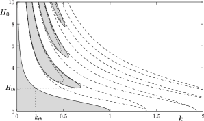
Figure 2: Stability chart in the plane spanned by the dimensionless wavenumber $k$ and the magnetic field amplitude $H_{0}$ for the flat interface between a ferrofluid and a non-magnetic fluid in a rotating magnetic field. The dimensionless angular frequency of the magnetic field is $\Omega=0.69$ corresponding to $f=10\,{\rm Hz}$, the remaining parameters are as given in the main text. The full lines separating the white regions of stability from the gray regions of unstable combinations derive from a numerical solution of (47). For comparison also the results of the inviscid theory building on (49) and of the approximate treatment of viscosity related to (50) are included as long and short dashed lines respectively. The threshold values of the magnetic field and wave number are $H_{th}=2.2$ and $k_{th}=0.2$ corresponding in physical units to $H_{th}\simeq 7.3\,{\rm kAm^{-1}}$ and $\lambda_{th}\simeq 3.7\,{\rm cm}$.

In this section we display detailed results of our analysis for a typical experimental combination of a ferrofluid and an immiscible non-magnetic fluid which has been used in a related experimental investigation Pacitto . The fluid parameters are as follows: $\rho^{(2)}=1690\,{\rm kg\,m^{-3}}$, $\eta^{(2)}=0.14\,{\rm Pa\,s}$, $\chi=2.6$, $\rho^{(1)}=800\,{\rm kg\,m^{-3}}$, $\eta^{(1)}=0.005\,{\rm Pa\,s}$, and $\sigma=0.012\,{\rm N\,m^{-1}}$. For the capillary length $\lambda_{c}=2\pi/k_{c,H=0}$ we then obtain $\lambda_{c}\simeq 7\,{\rm mm}$. The dimensionless magnetic field amplitude $H_{0}=1$ corresponds to a field of $H_{0}=3.3\,{\rm kA/m}$, $\Omega=1$ corresponds to a field rotating with frequency $f=14.6\,{\rm Hz}$.

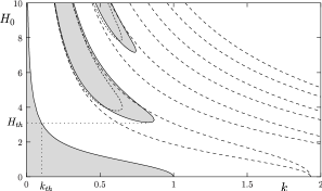
Figure 3: Same as Fig. 2 for an angular frequency of $\Omega=1.37$ ($f=20\,{\rm Hz}$). Due to the higher frequency the influence of the viscosity is stronger giving rise to the threshold values $H_{th}=3.1$ and $k_{th}=0.1$ corresponding to $H_{th}\simeq 10.3\,{\rm kAm^{-1}}$ and $\lambda_{th}\simeq 7.4\,{\rm cm}$.

In Figs. 2 and 3 we show the regions of instability of the flat interface in the $k$-$H_{0}$ plane. For $H_{0}=0$ all perturbations are unstable for which the modulus of the wave vector is smaller than 1 (in our dimensionless units, cf. (15)), which is the well-known trademark of the Rayleigh-Taylor instability. Increasing $H_{0}$ from zero the interval of unstable wave numbers shrinks and hence more and more long-wave perturbations may be stabilized. However, if $H_{0}$ gets larger than a threshold value $H_{th}$ the parametric excitation due to the time-dependent magnetic field gives rise to new instabilities at higher wave-numbers. Since these additional unstable modes are clearly unwanted $H_{0}$ must remain below this threshold value $H_{th}$. Correspondingly there is a threshold $k_{th}$ for the wavenumber modulus such that perturbations with $k<k_{th}$ cannot be stabilized with the help of the magnetic field. As we will detail in section VII these modes have to be stabilized by lateral boundary conditions. We note that with decreasing $\Omega$ the tongues of instability move closer together and come nearer to the $k$-axis implying $H_{th}\to 0$ and $k_{th}\to 1$ for $\Omega\to 0$.

It is clearly seen from the figures that the stability regions are strongly influenced by the viscosity of the liquids. In the inviscid theory the tongues of instability all reach the $k$-axis implying that any rotating magnetic field would induce new unstable modes at values of $k$ that were stable in the absence of the field. Therefore a complete suppression of the Rayleigh-Taylor instability would be impossible. It is also apparent that for realistic parameter combinations the phenomenological inclusion of viscosity in the theoretical description as discussed in the previous section may give results which significantly differ from the complete theory. This is similar to the analysis of the Faraday instability performed in KumarTuckerman .

Figs. 4 and 5 display the dependence of the threshold values $H_{th}$ and $k_{th}$ on the angular frequency $\Omega$ of the field. Clearly $H_{th}$ increases and $k_{th}$ decreases with increasing $\Omega$ as exemplified also by a comparison between Fig. 2 and 3. For the parameters considered an increase in $\Omega$ beyond $\Omega=2$ does not significantly reduce $k_{th}$ any more.

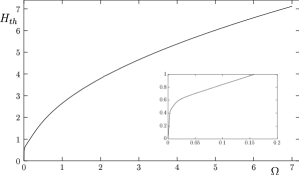
Figure 4: Threshold value $H_{th}$ of the magnetic field amplitude $H_{0}$ as function of the angular frequency $\Omega$ of the field for the parameters given in the main text. The displayed interval $\Omega=1...7$ corresponds in physical units to $f\simeq 15\,{\rm Hz}...100\,{\rm Hz}$. The inset shows a blow-up of the steep increase of $H_{th}$ for small values of $\Omega$.

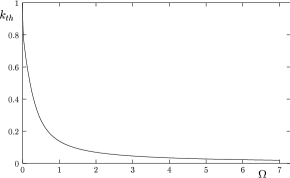
Figure 5: Similarly to Fig. 4 the threshold value $k_{th}$ of the wavenumber modulus $k$ is shown as function of the angular frequency $\Omega$ of the field.

Finally, Fig. 6 combines Figs. 4 and 5 and shows the relation between the two threshold values $H_{th}$ and $k_{th}$.

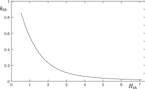
Figure 6: Threshold value $k_{th}$ of the wave number $k$ versus threshold value $H_{th}$ of the magnetic field amplitude $H_{0}$, again for the special set of parameters given in the main text.

VII Discussion

In the present paper we have investigated the possibility to stabilize a layering of a ferrofluid and a non-magnetic fluid which were potentially unstable due to the Rayleigh-Taylor instability by a spatially homogeneous magnetic field rotating in the plane of the undisturbed interface. Special emphasis was put on an exact treatment of the influence of the viscosities by starting from the complete set of Navier-Stokes equations for both liquids. Our results show that this approach is for experimentally relevant parameter values superior to both the inviscid theory and to a standard phenomenological procedure to include viscous effects using the inviscid flow field.

The trademark of the Rayleigh-Taylor instability is a band of unstable wave numbers extending from $k=0$ up to a threshold value $k_{th}$ which in the absence of magnetic effects is given by the capillary wavelength $k_{c}=\sqrt{\triangle\rho g/\sigma}$. The main result of the present investigation is that $k_{th}$ may be reduced roughly by a factor of ten with the help of a rotating magnetic field of experimentally easily accessible amplitude and frequency. As expected the stabilization works best for ferrofluids with high susceptibility $\chi$ which, however, have also high densities increasing in turn $k_{c}$.

In order to provide a clean initial condition for an experimental study of the onset of the Rayleigh-Taylor instability one has also to stabilize the modes with $k\leq k_{th}$. One way to accomplish this suppression may be to use the boundary condition of a finite geometry, i.e. by pinning the contact line between the liquids at the boundary of the sample. In this way all long wave-number modes with $k<k_{bc}$ are stabilized. Here $k_{bc}$ is determined by the linear extension $L$ of the sample and roughly given by $k_{bc}\simeq\pi/L$. Modes with $k>k_{c,H=0}$ are suppressed by surface tension. If one is able to temporarily stabilize the remaining modes by the rotating magnetic field, i.e. if one is able to realize $k_{th}<k_{bc}$ the flat interface is stable. Switching off the magnetic field at a given time all modes with $k_{bc}<k<1$ will become unstable. Since it is easily possible to realize values of $k_{th}$ significantly smaller than $k_{max}$, the wavenumber with largest growth rate in the absence of the field, the ensuing Rayleigh-Taylor instability should closely resemble the case without lateral boundary conditions. To be precise it should be emphasized that our theoretical analysis is for infinite layers only and does not take into account the influence of lateral boundary conditions. However, the relevant values of $H_{th}$ and $k_{th}$ will only marginally be modified.

For an order of magnitude estimate let us consider a cylindrical vessel of diameter $d=5\,{\rm cm}$. Pinning the contact line at the boundary the instability of modes with dimensionless wavenumber $k<k_{bc}\simeq 0.11$ will be suppressed. On the other hand a rotating magnetic field with amplitude $H_{0}\simeq 10\,{\rm kAm^{-1}}$ and frequency $f=20\,{\rm Hz}$ realizes $k_{th}\simeq 0.1$ (cf. Fig. 3). Switching off the magnetic field all modes with $k_{bc}<k<1$ will become unstable. For the above example this includes the first 8 cylindrical modes which should allow a rather accurate study of the Rayleigh-Taylor instability. We hope that our theoretical study may stimulate experimental work along these lines.

- (1) Lord Rayleigh, Scientific Papers (Cambridge University Press, Cambridge, England, 1900) 2, pp. 200-207
- (2) G. I. Taylor, Proc. R. Soc. London, Ser. A 201, 192 (1950)
- (3) D. J. Lewis, Proc. R. Soc. London, Ser. A 202, 81 (1950)
- (4) S. Chandrasekhar, Hydrodynamic and Hydromagnetic Stability, (Oxford University Press 1961)
- (5) D. H. Sharp, Physics D12, 3 (1984)
- (6) P. F. Linden and J. M. Redondo, Phys. Fluids A3, 1269 (1991)
- (7) S. B. Dalziel, P. F. Linden, and D. L. Youngs, J. Fluid. Mech. 399, 1 (1999)
- (8) M. S. Plesset and C. G. Whipple, Phys. Fluids 17, 1 (1974)
- (9) A. Lange, M. Schröter, M. A. Scherer, and I. Rehberg, Eur. Phys. J. B 4, 475 (1998)
- (10) G. H. Wolf, PRL 24, 9 (1970)
- (11) G. H. Wolf, Z. Physik A 227, 291 (1969)
- (12) J. M. Burgess, A. Juel, W. D. McCormick, J. B. Swift, and H. L. Swinney, PRL 86, 1203 (2001)
- (13) R. E. Rosensweig, Ferrohydrodynamics, Cambridge University Press, Cambridge, (1985)
- (14) M. D. Cowley and R. E. Rosensweig, J. Fluid Mech. 30, 671 (1967).
- (15) G. Pacitto, C. Flament, J.-C. Bacri, and M. Widom, PRE 62, 7941 (2000)
- (16) P. Carlès, Z. Huang, G. Carbone, and C. Rosenblatt, PRL 96, 104501 (2006)
- (17) R. E. Zelazo, and J. R. Melcher, J. Fluid Mech. 39, 1 (1969)
- (18) D. W. Jordan, and P. Smith, Nonlinear ordinary differential equations, 3th edition, Oxford University Press, Oxford (1999)
- (19) K. Kumar, and L. S. Tuckerman, J. Fluid. Mech. 279, 49 (1994); K. Kumar, Proc. Soc. Lond. A 452, 1113 1996
- (20) Y. Fautrelle and A. D. Sneyd, J. Fluid. Mech. 375, 65 (1998)
- (21) T. Mahr, and I. Rehberg, Europhys. Lett. 43, 23 (1998)
- (22) M. Abramowitz, I.A. Stegun, Handbook of mathematical functions, (Dover Publications, Inc., New York, 1972)
- (23) H. Lamb, Hydrodynamics, 6th edition, (Dover, New York, 1932), §348
- (24) L. D. Landau and E. M. Lifschitz, Hydrodynamik, (Akademie-Verlag, Berlin, 1991), §25