Experimental evidence of accelerated energy transfer in turbulence

Abstract

We investigate the vorticity dynamics in a turbulent vortex using scattering of acoustic waves. Two ultrasonic beams are adjusted to probe simultaneously two spatial scales in a given volume of the flow, thus allowing a dual channel recording of the dynamics of coherent vorticity structures. Our results show that this allows to measure the average energy transfer time between different spatial length scales, and that such transfer goes faster at smaller scales.

Much of the investigation in turbulence has been devoted to the understanding of the mechanisms underlying the energy transfer through the turbulent cascade, a concept introduced by Richardson in 1922 Frisch . A good deal of theoretical and numerical work has been dedicated to study shell models, which include the essential features expected in a turbulent cascade, but without some of the complications inherent to the Navier-Stokes equations. Though these models retain some of the dynamics of the motion equations, they handle the velocity field as a scalar. Thus the price payed is a complete loss of flow geometry Bife . Another approach is the study of random multiplicative cascade models, which adequately mimic the statistics of the local energy dissipation rate $\epsilon$ at different flow scales, and the intermittency of small scales observed in a large number of experimental results. Although much progress was done, many issues related to the statistics of energy transfer, energy dissipation and small scale intermittency in turbulent flows still remain without satisfactory answers. In particular, the dynamics of the energy transfer through the turbulent cascade has been only recently addressed in some theoretical works Leve ; Benz , but this aspect of turbulent flows is still lacking experimental studies specifically addressing it.

In this note we report an experimental result, obtained for the case of a vortex embedded in a turbulent flow produced in air by two coaxial centrifugal fans, each facing the other and rotating at fixed angular velocities. This so-called von Kármán flow has been used in a number of experiments in turbulence All . When the fans rotate in the same direction with identical speeds, a strong vortex is produced between them LPF . The advantage of this configuration is that in a small volume we obtain an intense and well-defined coherent vorticity structure, surrounded by a fully turbulent background. Details of this setup are given in a previous work LP . The parameters used in this case are: diameter of fans: D = 30 cm, height of vanes: $h=2.2$ cm, distance between disks: $H=30$ cm, rotation speed: $f=30$ Hz, and diameter of central holes: $d=2.5$ cm. The fans were driven by two DC motors, powered by independent constant voltage sources allowing to keep the disk rotation within $1$% of the desired speed. Local measurements of the airflow speed were performed with a Dantec Streamline 90N10 frame housing a Constant Temperature Anemometer which drives a $5\thinspace\mu$m diameter and $2$ mm length platinum wire probe. A Streamline 90H02 Flow Unit was used to calibrate it. To produce and detect the sound waves, four circular Sell type electrostatic transducers Ank were used, each having an active surface diameter of 14 cm. Two B&K model 2713 power amplifiers drove the emitters. The receivers used custom made charge amplifiers, whose output were connected to two Stanford Research model SR830 lock-in amplifiers (LIA) through $2^{\textrm{nd}}$ order high-pass RC filters having cut-off frequencies of 7.5 kHz. The sine-wave output of each LIA internal generator was used as signal source for the corresponding emitter. The LIA output signals, comprising in-phase and quadrature components, were low-pass filtered by an IOTech Filter-488 $8^{\textrm{th}}$ order elliptic filter bank, using a cutoff frequency of 4 kHz. The resulting signal was digitized at 12.5 kS/s with a 16-bit resolution National Instruments AT-MIO-16X multifunction board, installed into a personal computer. A total of $2^{20}$ points per signal channel was collected in each of 77 data sets.

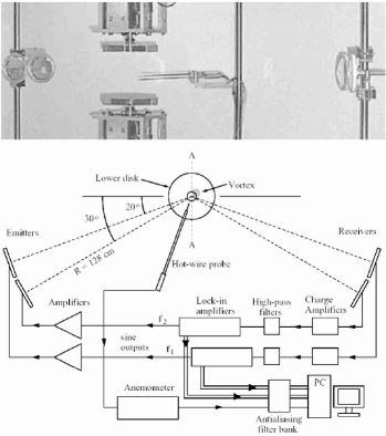
Figure 1: Top: Partial view of the experimental setup. Bottom: a schematic drawing of the experimental setup (see text).

Fig. 1 (top) shows the device that produced the flow, along with the four circular ultrasonic transducers, and the hot-wire probe. The transducers were arranged to perform measurements using an interferometric configuration, described in detail in a previous work Baud . The scattering angles were $\theta_{1}=40^{\circ}$ and $\theta_{2}=60^{\circ}$. The magnitude of the scattering wave-vectors, $q_{i}^{scatt}=4\pi\nu_{0,i}\sin(\theta_{i}^{scatt}/2)/c=|\bm{k^{\prime}}-\bm{k}|,i=1,2$, were adjusted independently for each channel through their corresponding frequencies $\nu_{0,i}$. We acquired three sets of data, setting $\nu_{0,1}=20$ kHz, $40$ kHz, and $60$ kHz; while $\nu_{0,2}$ took some 25 values in the interval $[16,90]$ kHz in each case. Notice that each probed scattering wave-vector, related to the $z$ -component of the vorticity distribution, can be set arbitrarily close (even identical) to the other. Fig. 1 (bottom) displays a schematic upper view of the lower disk, hot-wire probe and ultrasonic transducers, along with distances and angles. This arrangement is symmetric with respect to the vertical plane AA. Also displayed is a schematic diagram of the measuring chain. Fig. 2 (top) is a sketch of the volume probed by the ultrasonic beams, showing the relationships between scattering vectors and wave-vectors in the case of exact inter-channel tuning (same scattering wave-vector). As mentioned in previous works LPF ; LP , the vortex performs a slow precession motion around the axis of rotation of the fans. Even so, it remains inside the measurement volume, as shown in fig. 2. A horizontal cut of the measurement volume is displayed as a shaded rhombus, the heavier shaded circle indicating the position of the vortex core. Air speed measurements with the probe wire aligned vertically, and located at about 2 cm of the disks’s rotation axis and some 10 cm above the lower disk, give the sample record displayed in fig. 2 (bottom). The nearly periodic precession of the vortex is visible as a pattern with sharp dips —sometimes enlarged or doubled by fluctuations due to the turbulent background, each time the center of the vortex is close or coincides with the hot wire location. These events are signaled by arrows in fig. 2, the time interval between single events being about $1$ s. Accordingly, the spectrum displayed in fig. 3 (top) has a rather wide peak located at $f_{0}\approx 1$ Hz. The Taylor hypothesis is not met by this flow, but this spectrum gives an idea of the energy contents at different scales. At higher frequencies (smaller scales), it meets only approximately the $k^{-5/3}$ K41 law (represented by the straight line) in the inertial range, due to the presence of the vortex in the bulk of the flow. In fact, we observe three regions, A, B, and C, where the spectrum looks self-similar, but with different slopes. As we will see later, this could be related to the influence of the flow anisotropy on the dynamics of the energy transfer through the turbulent cascade. The acoustic signals are delivered by the LIAs as low frequency complex voltages, which are images of the spatial Fourier modes $\Omega_{z}(q_{j},t)$ of the flow vorticity, probed at well-defined wave vectors $q_{j}=4\pi\nu_{0,j}\sin(\theta_{j}/2)/c$, $j=1,2$. Typical spectra of these signals are displayed in fig. 3 (bottom). The wide central peak, due to the intense coherent vorticity of the vortex, lies between two side bands produced by the background flow. There is a close correspondence between the low frequency region of the velocity spectrum (up to $50$ Hz) and the central region of the vorticity spectrum. The same is true for the high frequency region ($>200$ Hz) of the spectra, both exhibiting a slowly decaying roll-off, with a slope close to $-5/3$ related to the background turbulence of the flow.

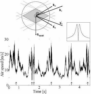
Figure 2: Top: Diagram showing the relationship between wave-vectors, the volume probed by the ultrasonic beams (shaded region) and the size of the disks. The dark circle represents a cut of the vortex core. Bottom: A sample of the anemometer signal. Arrows signal events of minimal air speed, the vortex core being close to the hot wire probe there. The inset displays the velocity profile of a non turbulent vortex, which helps in recognizing the vortex core in the turbulent signal.

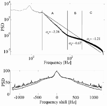
Figure 3: Top: Power spectral density of the signal displayed in fig. 2. Three almost linear regions are labeled A, B, and C (see text), with slopes $\alpha_{A,B,C}$. The straight line represents the Kolmogorov spectrum, with slope $\alpha_{K}=-1.66$. Bottom: Individual spectra of the signals delivered by the lock-in amplifiers. The spectrum corresponding to the scattering angle of 60 degrees decreases slightly faster with the frequency shift. Scattered waves having the same central frequency of the incident beam have no frequency shift.

Now we address the separation of the coherent structure and the background turbulent flow. Following ref. Baud , we compute the coherence between two spatial Fourier modes of the vorticity, $\Omega_{z}(q_{1},t)$ and $\Omega_{z}(q_{2},t)$. The coherence function, $C(q_{1},q_{2},\nu)=\langle\Omega_{z}(q_{1},\nu)\Omega^{\ast}_{z}(q_{2},\nu)\rangle/\sqrt{\langle|\Omega_{z}(q_{1},\nu)|^{2}\rangle\langle|\Omega_{z}(q_{2},\nu)|^{2}\rangle}$, where $\nu$ is a frequency shift associated to the Fourier transform in time of $\Omega_{z}(q_{i},t)$, is a statistical estimator that allows to evidence phase stationarity (coherence) between distinct Fourier modes. Fig. 4 (top) is a plot of the coherence between two scattering channels tuned to probe the same scale of the vorticity distribution $(q_{1}=q_{2})$. A central peak with a high level of coherence ($0.9$, being $1$ the maximum expected value; the value of $0.9$ should be ascribed to incoherent noise) reveals that both channels are detecting the same coherent structure. This was verified “turning off” the vortex by rotating the disks in opposite directions at the same angular speed. In this case only a turbulent shear layer remains, and the plot of the coherence function displays only the side bands. By stacking plots of coherence for a sequence of values of $q_{1}$, it is possible to build surfaces of coherence relating events at different flow scales, as functions of $\Delta q=q_{2}-q_{1}$ and the frequency shift $\nu$, as shown in fig. 4. We can interpret them in as eddies at given scales drawing its energy from decaying structures at larger scales, in the frame of the Richardson’s turbulent cascade. As these surfaces represent a time average of the whole story, we perform a time cross-correlation analysis to confirm this interpretation. This is done by computing the cross-correlation $\chi(q_{1},\Delta q,\Delta t)=\langle|\Omega_{z}(q_{1},t)||\Omega_{z}(q_{1}+\Delta q,t+\Delta t)|\rangle/\sqrt{\langle|\Omega_{z}(q_{1},t)|^{2}\rangle\langle|\Omega_{z}(q_{1}+\Delta q,t+\Delta t)|^{2}\rangle}$, were $|\Omega_{z}(q_{i},t)|$ is a measure of the strength of a structure with vorticity $\Omega_{z}(q_{i},t)$. The function $\chi(q_{1},\Delta q,\Delta t)$ will have a peak at $\Delta t=\tau$ ($\tau=$ time lag), indicating the presence of a vorticity pattern at the scale $l_{1}=2\pi/q_{1}$ in time $t$ that appears at the scale $l_{2}=2\pi/q_{2}$ a time $t+\tau$ later. The peak amplitude is a measure of how well the pattern is preserved from one scale to the other, a value of one meaning a perfect preservation. Fig. 5 shows three straight lines resulting from fits to the time lags calculated from such cross-correlation analysis, each corresponding to one of the coherence surfaces shown in fig. 4. The time lags found here are consistent with those given in reference Baud . We have $\tau\sim 1$ ms for $\Delta q=8$ cm^-1, and the transfer rates of fig. 7 (c) in reference Baud are similar note .

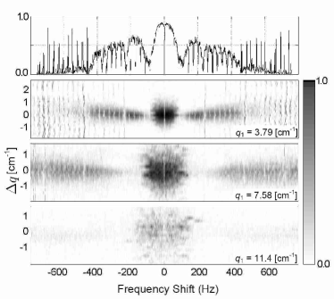
Figure 4: Top: coherence plot of signals detected simultaneously by both receivers. The wide peak centered at zero frequency shift is due to the vortex. Bottom: Three coherence surfaces are shown, obtained by detuning one of the emitters by a frequency corresponding to a shift $\Delta q$ in the wave number.

Our main result is the experimental observation of acceleration in the energy transfer in turbulence, evidenced by the systematic change in the trend of the data in fig. 5 when the magnitude of the reference wave-vector $q_{1}$ is changed. The slopes of the fitted straight lines decrease with increasing $q_{1}$. The scattering of the points is an indication of the intrinsic variability of the energy transfer time through the turbulent cascade ($R^{2}\geq 0.6$ in all cases). The following argument helps to understand the trend change: the time lag measured between the wave numbers $q_{1}$ and $q_{2}=q_{1}+\Delta q$ can be seen as the average transfer time of the energy contained in a scale corresponding to $q_{1}$ to a smaller scale corresponding to $q_{2}$. Thus, the slope $\delta\tau/\delta q$ (we drop $\Delta$’s from now on) of the straight lines can be related to the inverse of the average transfer rate of energy in the $k$ -space, in a neighborhood of the reference scale corresponding to the wave number $q_{1}$ Fauve . This decrease in slope with increasing $q_{1}$ reveals that the average transfer time of the energy decreases when the involved scales are smaller. In other words, taking $\delta q/\delta\tau$ as the average transit speed (in the $k$ -space) of structures starting at the wave number $q_{1}$ and ending at the wave number $q_{2}$, we conclude that such speed is larger at larger $q$’s (or smaller scales). This is consistent with a remark made in a previous numerical work Leve . A rather crude explanation of this result follows: if $E(q)$ is the spectral density of energy per unit mass —averaged in time, and we think of $\delta q/\delta\tau$ as being an ordinary derivative, then $E(q)\delta q/\delta\tau$ is the average energy flux density in $k$ -space. But this is the average dissipation rate per unit mass $\epsilon$. Thus, $E(q)\delta q/\delta\tau=\epsilon$, and $\delta\tau/\delta q=E(q)/\epsilon$. As $E(q)$ decreases with increasing $q$, so does $\delta\tau/\delta q$. Notice that in this picture, the energy attached to a given eddy is transported towards larger wave numbers merely by reduction of its spatial scale (in directions perpendicular to its vorticity) due to stretching by the velocity field of larger eddies.

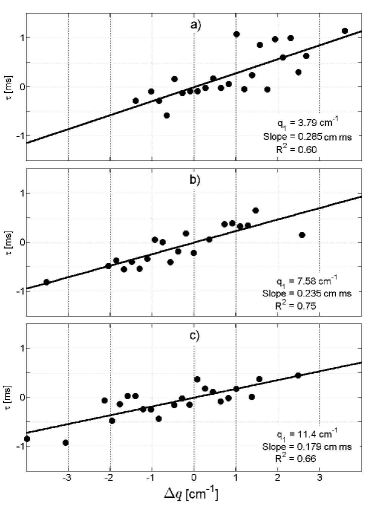
Figure 5: Time lags corresponding to the coherence surfaces of fig. 4. a), b), and c) correspond to $q_{1}=3.79,~{}7.58,$ and $11.4$ cm^-1, respectively. The straight lines are linear fits to the measured points, with correlation coefficient $R^{2}=0.60~{}(0.75,0.66)$. Note that the slopes decrease with increasing $q_{1}$.

We can illustrate our view in the frame of K41 theory Frisch : we have $E(q)=C_{\text{K}}\epsilon^{2/3}q^{-5/3}$, where $C_{\text{K}}$ is the Kolmogorov constant. Thus, for homogeneous and isotropic turbulence, $\delta\tau/\delta q=C_{\text{K}}\epsilon^{-1/3}q^{-5/3}$, which is of course a decreasing quantity. By rearranging terms, we have $q^{-5/3}\delta q=(\epsilon^{1/3}/C_{\text{K}})\delta t$, which by integration yields $q(t)=(q_{0}^{-2/3}-\frac{2}{3}\epsilon^{1/3}t/C_{\text{K}})^{-3/2}$. This is the itinerary of the average magnitude $q$ in a homogeneous and isotropic turbulent flow in which the mean dissipation rate per unit mass is $\epsilon$. The scale $l_{0}=2\pi/q_{0}$, corresponding to $t=0$, can take any value within the inertial range. Notice that $q(t)$ diverges in a finite time $t_{\text{K}}^{0}=\frac{3}{2}C_{\text{K}}\thinspace\epsilon^{-1/3}q_{0}^{-2/3}$, corresponding to the average time taken by the energy at the scale $l_{0}$ to cascade down to $l=0^{+}$ ($q\rightarrow\infty$), in a fluid with vanishing viscosity —in the frame of K41 theory. Putting $C_{\text{K}}\approx 0.5$, $\epsilon\sim 10^{2}$ W/kg, estimated from the power injected to the flow ($\approx 70$ W) and the volume of moving air ($\sim 0.5$ m³) and, for instance, $q_{0}\approx 3\times 10^{2}$ m^-1, corresponding to the largest scale measured with our acoustic method, we get $t_{\text{K}}^{0}\sim 4$ ms. This is on the order of characteristic times in fig. 5, showing that transfer times in homogeneous turbulence do not differ too much from those in our flow. Thus, our reasoning shows that the trend observed in fig. 5 can be understood in terms of “classical” homogeneous and isotropic turbulence. In non-homogenous, non-isotropic turbulence, as in the present experiment, the behavior of $\delta\tau/\delta q$ can be estimated from the experimental spectrum shown in fig. 3, where the Kolmogorov spectrum is plotted as a straight line, for comparison. In the large scales region (A), $\delta\tau/\delta q$ decreases faster than in K41 turbulence, the cascade acceleration being larger. In the small scales region (C), $\delta\tau/\delta q$ tends to reach the Kolmogorov slope, but the acceleration is slightly smaller than in K41. Region (B), in which the cascade acceleration reaches its minimum, is a transition zone from a non-isotropic flow at large scales, where vorticity is mainly parallel to the $z$ -axis, to a more isotropic small-scale flow. In all three regions the spectrum seems to be self-similar, with different scaling exponents. Of course, being this one a first experimental result revealing the accelerated nature of energy transfer through the turbulent cascade, more work will be necessary to state our conclusions on more solid ground. We recall that we are measuring only the $z$ -component of the vorticity and the modulus of the velocity component normal to the $z$ -axis. It should be necessary to simultaneously measure at least one more component of the vorticity. Additionally, the conditions of validity for the Taylor hypothesis are not meet in these hot-wire measurements —a flying probe would be much better to study this flow. At any rate, in the large-scale range the vorticity in our flow is mainly parallel to the $z$ -axis. Thus, eddies in the large scale region have mostly parallel vorticities, and the vortex stretching is largely inhibited there, slowing down the energy transfer. At smaller scales, where a more isotropic flow exists, vortex stretching is reestablished, giving faster energy flux rates. Thus, in-between the acceleration should be greater than in the isotropic case. This could explain in part our results. To conclude, we remark that our reasoning suggest that cascade acceleration may be a necessary but not sufficient condition for small scale intermittency.

Financial support for this work was provided by FONDECYT, under projects #1990169, #7990057 and #1040291.

References

- (1) U. Frisch, Turbulence: the Legacy of A. N. Kolmogorov, (Cambridge University Press, Cambridge, 1995)
- (2) L. Biferale, Annu. Rev. Fluid Mech. 35, 441 (2003)
- (3) E. Lévêque and C. R. Koudella, Phys. Rev. Lett. 86, 4033 (2001).
- (4) Roberto Benzi, Luca Biferale, and Mauro Sbragaglia Phys. Rev. E 71, 065302(R) (2005).
- (5) For example, experimental results in confined von Kármán flows are given in J.-F. Pinton, P. C. W. Holdsworth, and R. Labbé, Phys. Rev. E 60, R2452 (1999); P. Odier, J.-F. Pinton, and S. Fauve, Phys. Rev. E 58, 7397 (1998); O. Cadot, Y. Couder, A. Daerr, S. Douady, and A. Tsinober Phys. Rev. E 56, 427 (1997); O. Cadot, S. Douady, and Y. Couder, Phys. Fluids 7, 630 (1995); J. Maurer, P. Tabeling, and G Zocchi, Europhys. Lett. 26, 31 (1994); S. Douady, Y. Couder, and M. E. Brachet, Phys. Rev. Lett. 67, 983 (1991).
- (6) R. Labbé, J.-F. Pinton, and S. Fauve, Phys. Fluids 8, 914 (1996).
- (7) R. Labbé and J.-F. Pinton, Phys. Rev. Lett. 81, 1413 (1998).
- (8) C. Baudet, O. Michel, and W. J. Williams, Physica D 128, 1 (1999).
- (9) D. Anke, Acustica 30, 30 (1974).
- (10) We have not dropped factors here in the magnitude of scattering vectors, which explain the difference in scales in the aforementioned figures.
- (11) This is like measuring the advection of a magnitude in the Fourier space. Of course, here the “advection” mechanism lies in the dynamics of the turbulent velocity field in the direct space. The idea of measuring a wind in the Fourier space by looking simultaneouly at two different scales was proposed by S. Fauve in 1990.