A method for extracting the scaling exponents of a self-affine, non-Gaussian process from a finite length timeseries.

Abstract

We address the generic problem of extracting the scaling exponents of a stationary, self-affine process realised by a timeseries of finite length, where information about the process is not known a priori. Estimating the scaling exponents relies upon estimating the moments, or more typically structure functions, of the probability density of the differenced timeseries. If the probability density is heavy tailed, outliers strongly influence the scaling behaviour of the moments. From an operational point of view, we wish to recover the scaling exponents of the underlying process by excluding a minimal population of these outliers. We test these ideas on a synthetically generated symmetric $\alpha$-stable Lévy process and show that the Lévy exponent is recovered in up to the $6^{th}$ order moment after only $\sim$0.1-0.5% of the data are excluded. The scaling properties of the excluded outliers can then be tested to provide additional information about the system.

I introduction

There is increasing observational evidence that natural systems often show scaling in a statistical sense, coincident with non-Gaussian ‘heavy tailed’ statistics. Complex systems approaches aim to understand these phenomena as universal, with a key quantitative prediction of theory being scaling exponents. Importantly, the identification of universal scaling functions implies the ability to describe many different length and time scales as well as apparently disjoint physical phenomena with the same macroscopic scaling behaviour Sethna et al. (2001); Sornette (2000); Mandelbrot (1983).

One of the outstanding challenges in complex system science is then to find robust methods that (i) establish whether there is scaling and (ii) accurately determine the scaling exponents for statistical measures of series of data that are of large, but finite length. We seek to determine the scaling properties of probability distributions that are heavy-tailed. The scaling exponents can be determined through the scaling behaviour of the moments, usually characterised by computing structure functions. Where the probability density is heavy tailed the moments and structure functions can depend strongly on extremal values, or outliers. Once we insist that the data series is represented by a finite number of measurements, the values at which these outliers occur will always vary between one realisation and the next. From an operational point of view, that is, when the underlying behaviour is not known a priori, these outliers can potentially distort the scaling properties of the data and the values of scaling exponents extracted via the structure functions. In this paper we propose a generic method for excluding these outliers in a manner which does not distort the underlying scaling properties of the data. These outliers also contain information and we explore a method for extracting this. We will test these ideas on numerically generated Lévy processes.

There has been considerable interest in fractional kinetics as providing stochastic models for the data of candidate complex systems Zaslavsky (2002); Schmitt et al. (1999). Lévy processes have been identified for example in biological systems (foraging of albatrosses Viswanathan et al. (2002)), financial markets (S&P 500 Mantegna and Stanley (1995)) and physical systems (laser cooling and trapping Bardou et al. (2002)). A robust method for determining the Lévy exponent from finite sized data sets, where the statistics are not known a priori is thus important in its own right. The method that we propose here is however quite generic, with application to a wide class of systems that show scaling; for example those that can be modelled by stochastic differential equations with scaling Hnat et al. (2003, 2005); Chapman et al. (2005). In this wider context Lévy processes, which have non-convergent higher order moments, provide a particularly stringent test of our ideas.

I.1 Statistical self-similarity

One can characterise fluctuations in a timeseries $x(t)$ on a given time scale $\tau$ in terms of a differenced variable $y(t,\tau)$

$$y(t,\tau)=x(t+\tau)-x(t)\ ,$$ (1)

for time $t$ and interval $\tau$, where the timeseries/stochastic process $x(t)$ represents a particular realisation or set of observations of the system from which the $y$’s are generated. We consider the case where the $y(t,\tau)$ satisfy the following scaling relation

$$y(b\tau)\,{\buildrel d\over{=}}\,f(b)y(\tau)\ ,$$ (2)

where $b$ is some scale dilation factor; $\,{\buildrel d\over{=}}\,$ indicates an equality in the statistical/distribution sense; $f$ is some scaling function (to be determined); and we have dropped the time argument in the increments $y$ by assuming statistical stationarity. Both $b$ and $f(b)$ are positive. The property in (2) is a generalized form of self-affinity, and in this sense $x(t)$ is a self-affine field. Self-affinity is a particular case of statistical self-similarity i.e. stochastic processes that exhibit the absence of characteristic scales Mandelbrot (1983); Greis and Greenside (1991); Chapman et al. (2005). We can write the scaling transformations (2) as

$$\tau^{\prime}=b\tau\ ,\quad\;y^{\prime}=f(b)y\ ,$$ (3)

where the primed variables represent scaled quantities. Conservation of probability under change of variables implies that the probability density function (PDF) of $y$, $P(y,\tau)$ is related to the PDF of $y^{\prime}$, $P(y^{\prime},\tau^{\prime})$ by

$$P(y,\tau) = P^{\prime}(y^{\prime},\tau^{\prime})\left|\frac{dy^{\prime}}{dy}\right|\ ,$$ (4)

thus giving from (3)

$$P(y,\tau)=f(b)P^{\prime}(f(b)y,\tau^{\prime})\ .$$ (5)

The result (5) expresses the fact that the stochastic process $x(t)$ is statistically self-similar i.e. that a given process on scale $\tau^{\prime}$ (and thus $y^{\prime}$) maps onto another process based on a different scale $\tau$ (and $y$) by the scaling transformation in (3); and that the PDFs of both these processes are related by (5).

We can go further and reduce the expression (5) to a function of one variable. Since the dilation factor $b$ is arbitrary we choose $b=\tau^{-1}$, which gives the important result

$$P(y,\tau) = f(\tau^{-1})P^{\prime}(f(\tau^{-1})y,1)$$ (6)

$$= f(\tau^{-1})\mathcal{P}_{s}(f(\tau^{-1})y)\ ,$$

and shows that any PDF $P$ of increments $y$ characterised by a time increment $\tau$ may be collapsed onto a single unique PDF $\mathcal{P}_{s}$ of rescaled increments $f(\tau^{-1})y$ and time increment $\tau=1$, by the above scaling transformation. Identification of this unique scaling function and the ensuing collapse is a clearer method of discriminating between different (universality) scaling classes than simply identifying the scaling exponents by themselves Sethna et al. (2001).

In this paper we will consider the scaling as defined by the structure functions. The generalised structure functions of order $p$ are simply defined as

$$S^{p}(\tau;\pm\infty)=\left\langle\left|y\right|^{p}\right\rangle\ =\int_{-\infty}^{\infty}\left|y\right|^{p}P(y,\tau)dy\ .$$ (7)

The analysis which follows is also valid for the moments; however, structure functions are typically calculated for data. This avoids the result that odd order moments of symmetric PDFs are zero so that as a consequence, in a physical system, they would be dominated by experimental error. Using the transformation (6), the scaling of the structure functions is:

$$S^{p}(\tau;\pm\infty) = \int_{-\infty}^{\infty}\left|y\right|^{p}P(y,\tau)dy$$ (8)

$$= \int_{-\infty}^{\infty}\left|y\right|^{p}f(\tau^{-1})\mathcal{P}_{s}(f(\tau^{-1})y)\ dy$$

$$\,{\buildrel{y^{\prime}=yf(\tau^{-1})}\over{=}}\, \left(f(\tau^{-1})\right)^{-p}\int_{-\infty}^{\infty}\left|y^{\prime}\right|^{p}\mathcal{P}_{s}(y^{\prime})\ dy^{\prime}$$

$$= \left(f(\tau^{-1})\right)^{-p}\mathcal{S}_{s}^{p}(1;\pm\infty)\ .$$

This formalism encompasses a general class of self-affine systems in the sense that it is not restricted to the well-studied case of mono-exponent scaling.

The above result (8) holds provided that the PDF $P$ is defined for all $y$. However, for finite data sets this is not the case. In this situation we have the integral (7) defined for the interval $[y_{-},y_{+}]$ where the $y_{\pm}$ are defined in some sense by the largest events measured in the data set. The values of $y_{\pm}$ will depend on the time scale $\tau$ and the sample size $N$ (which will be held constant). Thus the structure functions for the finite data set are

$$S^{p}(\tau;y_{\pm}(\tau))=\int_{y_{-}(\tau)}^{y_{+}(\tau)}\left|y\right|^{p}P(y,\tau)dy\ .$$ (9)

Manipulating this in a similar way to (8) results in the following scaling relation

$$S^{p}(\tau;y_{\pm}(\tau))=\left(f(\tau^{-1})\right)^{-p}\mathcal{S}_{s}^{p}(1;y_{\pm}(\tau)f(\tau^{-1}))\ .$$ (10)

If we assume that the values $y_{\pm}$ scale with $\tau$ in the same way as the increments $y$ in (3), then (10) becomes:

$$S^{p}(\tau;y_{\pm}(\tau))=\left(f(\tau^{-1})\right)^{-p}\mathcal{S}_{s}^{p}(1;y_{s\pm}(1))\ .$$ (11)

We will consider the case of self-affine scaling where the scaling function $f$ takes the form of a mono-scaling power law $f(b)=b^{H}=\tau^{-H}$, where $H$ is known as the Hurst exponent. Equation (6) then becomes

$$P(y,\tau)=\tau^{-H}\mathcal{P}_{s}(\tau^{-H}y)\ ,$$ (12)

and (8) becomes

$$S^{p}(\tau;\pm\infty)=\tau^{\zeta(p)}\mathcal{S}_{s}^{p}(1;\pm\infty)\ ,$$ (13)

where $\zeta(p)=Hp$ for this self-affine case. A log-log plot of $S^{p}$ vs. $\tau$ for various orders $p$ reveals scaling if present, and the slope of such a plot determines the exponents $\zeta(p)$ Sornette (2000); Bohr et al. (1998). One then verifies that $\zeta(p)=Hp$ by plotting $\zeta(p)$ as a function of $p$.

The aim of this paper is to obtain a good estimate of the scaling properties of (7), the structure functions at $N\rightarrow\infty$, via (11) for $N$ large but finite. However, we can anticipate that simply setting the limits $y_{\pm}$ of the integral (9) to the largest values found in a given realisation of the data, will give a scaling behaviour of (11) which can differ substantially from that of (13). This problem arises since the $y$ values of the extremal points fluctuate between one realisation and the next, and these fluctuations are more significant in heavy tailed distributions. This in turn will strongly modify the integral. We will therefore explore the possibility of choosing a range for the integral (9) based on the scaling property of the data itself, by systematically excluding the most extreme outlying points. This has the added advantage of not requiring a priori information about the system.

We stress that as our aim is to extract scaling exponents, we do not attempt to estimate the value of the moments or structure functions. Thus we will not compute an estimate of the integral (7) per se, rather we will examine methods for quantifying its dependence on the dilation factor $b$ (or equivalently $\tau$). Hence, our method can be applied to Lévy processes – where the moments are not defined, but where the PDF has scaling.

The paper is organised as follows. We first introduce the Lévy process that we will use to obtain (9) and briefly survey results pertaining to its asymptotic behaviour. We then discuss the effects of finite sized data sets and demonstrate the effect of removing outliers on the scaling behaviour of the Lévy process. We then explore the behaviour of these outliers.

II Lévy processes and Finite Size Effects

II.1 $\alpha$- stable processes

Many stochastic processes exhibit self-affine scaling and are characterised by ‘broad tails’ described by power-laws in their PDFs. Some possible mechanisms by which these power laws occur are discussed in Sornette (2000). This general class of stochastic processes can be described in the context of so-called $\alpha$-stable Lévy processes Samorodnitsky and Taqqu (1994); Zaslavsky (2002); Janicki and Weron (1994). We will restrict our attention to symmetric $\alpha$-stable processes. The PDFs $L_{\alpha}^{\gamma}$ of the increments $y$ of these processes are defined through the Fourier transform of their characteristic function

$$L_{\alpha}^{\gamma}(y,\tau)=\frac{1}{2\pi}\int_{-\infty}^{\infty}dke^{iky}e^{-\gamma\tau|k|^{\alpha}},$$ (14)

where $\gamma\geq 0$ and $\tau\geq 0$ are the characteristic scales of the process and describe the width of the distribution; and $\alpha\in(0,2]$ parameterises the stability of the distribution; $\alpha$ can be heuristically seen as an indication of the variability of the increments of such processes (also known as Lévy flights). In this paper we will take $\gamma=1$ and will consequently reduce the notation $L_{\alpha}^{\gamma}$ to $L_{\alpha}$. The form and convention of the parameters in equation (14) are similar to that presented in Paul and Baschnagel (1999); for a more rigorous discussion of the mathematical properties of such processes readers are referred to Samorodnitsky and Taqqu (1994); Janicki and Weron (1994).

From (14) it follows that the scaling properties of $L_{\alpha}$ are

$$L_{\alpha}(y,\tau) = \tau^{-\frac{1}{\alpha}}L_{\alpha}(\tau^{-\frac{1}{\alpha}}y,1)$$ (15)

$$= \tau^{-\frac{1}{\alpha}}\mathcal{L}_{s,\alpha}(\tau^{-\frac{1}{\alpha}}y)\ ,$$

from which the Hurst exponent of symmetric $\alpha$-stable processes is $H=1/\alpha$, by comparison with (12). Figure 1 (a) shows the $L_{\alpha}(y,\tau)$ for $\alpha=1.4$ and a range of $\tau=2^{0},2^{1},\ldots,2^{10}$; the scaling collapse (15) has been applied to these in Figure 1 (b).

a)

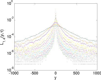
b)

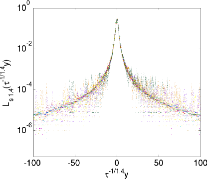
Figure 1: Plots showing probability density functions of the Lévy distribution for index $\alpha=1.4$ ($N=10^{6}$) at different values of differenced interval $\tau$ (a) before and (b) after the scaling collapse described by (15).

We now focus on the asymptotic behaviour of such distributions. By expanding the complex exponential in equation (14) and integrating one can show that in the large $y$ limit we obtain the asymptotic behaviour

$$\lim_{y\rightarrow\infty}L_{\alpha}(y,\tau) \simeq \frac{\tau\Gamma(1+\alpha)\sin(\pi\alpha/2)}{\pi\left|y\right|^{1+\alpha}}$$ (16)

$$= D_{\alpha}\frac{\tau}{\left|y\right|^{1+\alpha}}\ .$$

for $y\gg\tau^{\frac{1}{\alpha}}$ Paul and Baschnagel (1999); Jespersen et al. (1999). It immediately follows that these power-law tails ensure that for the $p^{th}$ moment to exist, $p-\alpha<0$. Hence the process has no variance defined for $0<\alpha<2$, and in the cases where $0<\alpha\leq 1$ the process will also have no mean defined i.e. both these quantities and the other higher order moments are infinite.

A generalized version of the Central Limit Theorem (CLT) Sornette (2000) ensures that the sum of all independent and identically distributed (i.i.d.) random variables with no finite variance that have distributions with power law tails that go asymptotically as $y^{-1-\alpha}$ ($\alpha\in(0,2]$), will converge to a Lévy distribution of the same index $\alpha$. In practice, however, we will always obtain a finite mean and variance from a finite length timeseries.

II.2 Finite-Size effects and outliers

We will now consider in detail the procedure for extracting the scaling exponents, $\zeta(p)$, from the structure functions in (13). This centres on first computing $S^{p}(\tau;y_{\pm})$ and the gradients $\zeta(p)$ of log-log plots of $S^{p}(\tau;y_{\pm})$ vs. $\tau$. If the process is self-affine ($\zeta(p)=Hp$) we should obtain a straight line on a plot of $\zeta(p)$ vs. $p$ from which we can measure the gradient and obtain the Hurst exponent, $H$. Note that the $\zeta(p)$ for several $p$ are needed to determine $H$ uniquely Chapman et al. (2005).

However, finite sample sizes result in pseudo multi-affine behaviour. As we will show, the primary reason for this anomalous behaviour is due to the large scatter in the outlying events of the tails of the distribution. In the case of Lévy-like processes this scaling bias shows up as a saturation/roll-over on the $\zeta(p)$ plots at $p>\alpha$.

a)

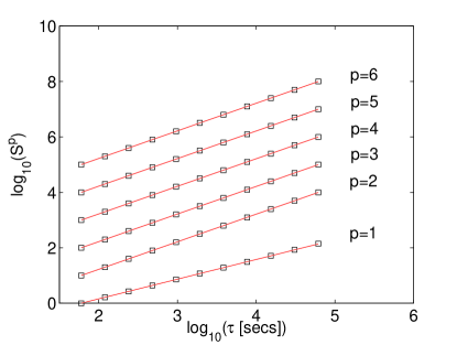
b)

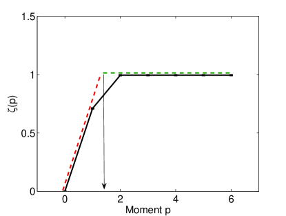
Figure 2: Plots of (a) generalised structure functions $S^{p}$ vs. $\tau$ for moments of order $p=1-6$, and (b) the scaling exponents $\zeta(p)$ vs. $p$ (solid black line). These quantities are shown for a Lévy process of index $\alpha=1.4$ and with $N=10^{6}$ data points. The dashed red line indicates the expected scaling $\zeta(p)=p/\alpha$ for $p<\alpha$; the green dashed line indicates the scaling exponent observed for $p>\alpha$ in a finite sized sample. The vertical arrow at $p\simeq\alpha$ seperates these two regions of scaling.

This can be seen in Figure 2 which illustrates both the methodology of extracting scaling exponents from structure function plots, and this finite sample size saturation effect in a Lévy process of index $\alpha=1.4$. This saturation effect is well-known and an explanation for it can be found in the work by Schmitt et. al. Schmitt et al. (1999) and Chechkin and Gonchar Chechkin and Gonchar (2000). We will now establish the scaling properties of these extremal events. We need to emphasise, however, that in contrast to Schmitt et al. (1999); Chechkin and Gonchar (2000) we will propose a method for estimating the integral in (7) such that the scaling in (13) is recovered for all $p$.

We consider the situation where we have many realisations, that is many data series of size $N$ obtained from the same process. Each of these realisations will have extremal points $y^{*}$ of their respective PDF. We know the properties of $\bar{y}^{*}$, the ensemble average of the $y^{*}$ over the realisations, since it will fall on the Lévy asymptotic distribution (16). We will use a simple example of Extreme Value Theory, EVT, (see Sornette (2000)) to obtain an estimate of the largest event in a sample of $N$ i.i.d. measurements of a random variable $y\in\mathbb{R}^{+}$. An approximation to the probability to see an event that occurs only once can be made by realising that an event with probability $P$ occurs typically $NP$ times. Therefore, the rarest event in a sample of $N$ measurements, which occurs typically only once can be seen to be described by $NP(y\geq\bar{y}^{*})=1$, where $P(y\geq\bar{y}^{*})$ is the probability of observing an event greater than or equal to $\bar{y}^{*}$ ; thus

$$P(y\geq\bar{y}^{*})=\frac{1}{N}\ .$$ (17)

We can generalise this to the $m^{th}$ largest event:

$$P(y\geq\bar{y}_{m}^{*})=\frac{m}{N}\ .$$ (18)

For the case of the Lévy-like process, within the limits of the integral in $P(y\geq\bar{y}_{m}^{*})$ the main contribution is from the tail and thus we can use (16) and estimate $P(y\geq\bar{y}_{m}^{*})$ to be

$$P(y\geq\bar{y}_{m}^{*})=\int_{\bar{y}_{m}^{*}}^{\infty}L_{\alpha}(y,\tau)dy\simeq D_{\alpha}\tau\int_{\bar{y}_{m}^{*}}^{\infty}\frac{dy}{\left|y\right|^{1+\alpha}}\ .$$ (19)

Evaluating the integral and equating with (18) gives the following result for the scaling behaviour of the $m^{th}$ largest event

$$\bar{y}_{m}^{*}=\left(\frac{D_{\alpha}N\tau}{m\alpha}\right)^{\frac{1}{\alpha}}\ .$$ (20)

A more detailed account would be to attempt to specify approximately the full PDF of the $m^{th}$ largest event amongst $N$ i.i.d. measurements. Following Sornette Sornette (2000) the cumulative distribution function (CDF) $\Pi(y<\bar{y}_{m}^{*})$ of the maximum value is

$$\Pi(y<\bar{y}_{m}^{*})=\int_{-\infty}^{\bar{y}_{m}^{*}}p_{N}(y)dy\simeq e^{-\frac{N}{m}P(y\geq\bar{y}_{m}^{*})}\ ,$$ (21)

where $p_{N}(y)$ is the PDF of the maximum value among $N$ observations, and is obtained by differentiating equation (21) to obtain

$$\frac{d\Pi(y<\bar{y}_{m}^{*})}{dy_{m}^{*}}=p_{N}(\bar{y}_{m}^{*})=\frac{N}{m}L_{\alpha}(\bar{y}_{m}^{*},\tau)e^{-\frac{N}{m}P(y\geq\bar{y}_{m}^{*})}\ .$$ (22)

By substituting (19) in (21) we obtain an estimate of the $m^{th}$ largest value, $\bar{y}_{m,\Pi}^{*}$, that will not be exceeded with probability $\Pi$. By setting the LHS of (21) to some probability $0<\Pi<1$, we obtain

$$\bar{y}_{m,\Pi}^{*}=\left(\frac{D_{\alpha}N\tau}{m\alpha\ln(1/\Pi)}\right)^{\frac{1}{\alpha}}\ .$$ (23)

If one was to set $\Pi=1/2$ the value of $y_{m}^{*}$ would correspond to the median value of the $m^{th}$ largest event. To obtain the modal value of $\bar{y}_{m}^{*}$ , we optimise for the maximum by differentiating (22) and setting it to zero. This gives us the following solution for the modal value of $\bar{y}_{m}^{*}$

$$\bar{y}_{m,mode}^{*}=\left(\frac{D_{\alpha}N\tau}{m(1+\alpha)}\right)^{\frac{1}{\alpha}}\ .$$ (24)

By comparing these expressions one can see that although the approximation of $\bar{y}_{m}^{*}$ becomes more refined, the scaling with $\tau$ is still that of (20). Thus we will proceed using the simplest expression (20). In addition, we will be working with a varying fraction $m/N$ rather than varying $m$ or $N$ separately. Importantly, since we are concerned primarily with the scaling with respect to $\tau$ we will write $\bar{y}_{m}^{*}$ more informatively as $\bar{y}_{m}^{*}(\tau)$ and thus adding to our scaling relations

$$\bar{y}_{m}^{*}(\tau)=\tau^{\frac{1}{\alpha}}\bar{y}_{m}^{*}(1)\ ,$$ (25)

as expected from equation (2) . We emphasise that this is the scaling of $\bar{y}_{m}^{*}$; the average over the $m^{th}$ largest events of a large number of realisations (timeseries). In practice we will have a single realisation and thus one value of $y_{m}^{*}$ which will fluctuate about this ensemble averaged $\bar{y}_{m}^{*}$. The behaviour (25) refers to the property that any point in the curve $P(y,\tau)$ scales as (6) and (3).

III Structure functions

III.1 Effects of finite sample size

We can now investigate the scaling behaviour of the structure functions of a Lévy-like process, but now with a finite sample size. Following the procedure in (11) we can discuss the structure functions in the average sense, that is averaged over many realisations of our $N$ sample finite length timeseries:

$$\bar{S}^{p}(\tau;\bar{y}_{1,\pm}^{*}(\tau)) = \int_{-\bar{y}_{1,-}^{*}(\tau)}^{\bar{y}_{1,+}^{*}(\tau)}\left|y\right|^{p}L_{\alpha}(y,\tau)dy$$

$$= \int_{-\bar{y}_{1,-}^{*}(\tau)}^{\bar{y}_{1,+}^{*}(\tau)}\left|y\right|^{p}\tau^{-\frac{1}{\alpha}}\mathcal{L}_{s,\alpha}(\tau^{-\frac{1}{\alpha}}y)\ dy$$

where we have set $m=1$ in $\bar{y}_{m}^{*}$ to emphasise that this is the structure function for the raw data with the largest events obviously bounding the data; the subscripts $+$ and $-$ indicate the largest positive and negative events. The substitution $y^{\prime}=\tau^{-\frac{1}{\alpha}}y$ gives

$$\bar{S}^{p}(\tau;\bar{y}_{1,\pm}^{*}(\tau)) = \tau^{\frac{p}{\alpha}}\int_{-\bar{y}_{1,-}^{*}(\tau)\tau^{-\frac{1}{\alpha}}}^{\bar{y}_{1,+}^{*}(\tau)\tau^{-\frac{1}{\alpha}}}\left|y^{\prime}\right|^{p}\mathcal{L}_{s,\alpha}(y^{\prime})\ dy^{\prime}$$ (27)

$$= \tau^{\frac{p}{\alpha}}\left[\int_{0}^{\bar{y}_{1,+}^{*}(\tau)\tau^{-\frac{1}{\alpha}}}y^{\prime p}\mathcal{L}_{s,\alpha}(y^{\prime})\ dy^{\prime}\right.$$

$$\ \left.+\int_{0}^{\bar{y}_{1,-}^{*}(\tau)\tau^{-\frac{1}{\alpha}}}y^{\prime p}\mathcal{L}_{s,\alpha}(y^{\prime})\ dy^{\prime}\right]\ .$$

To approximate the integrals in (27) we assume that values of the largest events are deep in the tail region of the distribution so that we may use the asymptotic form (16). This gives

$$\bar{S}^{p}(\tau;\bar{y}_{1,\pm}^{*}(\tau)) = \tau\ \frac{D_{\alpha}}{p-\alpha}\left(\bar{y}_{1,+}^{*(p-\alpha)}(\tau)+\bar{y}_{1,-}^{*(p-\alpha)}(\tau)\ \right)$$ (28)

$$\quad\quad\quad\quad\quad\quad\quad\quad\quad\quad\forall p>\alpha,$$

where the condition $p>\alpha$ is necessary as all structure functions of order $p<\alpha$ of a Lévy distribution exist (i.e. are finite) and this approximation would result in an infrared divergence in (27), which is clearly incompatible. For the ensemble average (19), (20) and (25) hold; thus we can simply substitute (25) into (28) to obtain:

$$\bar{S}^{p}(\tau;\bar{y}_{1,\pm}^{*}(\tau))=\tau^{\frac{p}{\alpha}}\ \frac{D_{\alpha}}{p-\alpha}\left(\bar{y}_{1,+}^{*(p-\alpha)}(1)+\bar{y}_{1,-}^{*(p-\alpha)}(1)\right)\ .$$ (29)

In practice the value of $y_{m}^{*}$ will vary for each realisation of $P(y,\tau)$ about the average $\bar{y}_{m}^{*}$ which obeys (25). For a given functional form of $P(y,\tau)$ the $y_{m}^{*}$ will have some probability density $p_{N}(y_{m}^{*})$ with a statistical spread about the average $\bar{y}_{m}^{*}$. An approximation to this can be made by substituting the asymptotic tail form of equation (16) into equation (22) to obtain

$$p_{N}(y_{m}^{*})=\frac{\Lambda}{y_{m}^{*1+\alpha}}\exp\left(-\frac{\Lambda}{\alpha y_{m}^{*\alpha}}\right)\ ,$$ (30)

where $\Lambda$ is given by

$$\Lambda=\frac{ND_{\alpha}\tau}{m}\ .$$ (31)

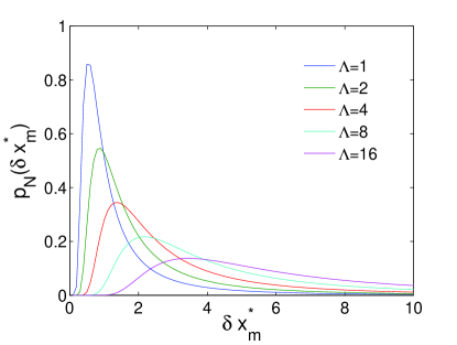
Figure 3: Plot showing the PDF, in equation (30), of the $m^{th}$ largest value of a sample size $N$ of a set of measurements taken from a Lévy-like process; the Lévy index $\alpha=1.5$.

Equation (30) is of the form of a stretched exponential. As with any power-law tailed PDF it has infinite variance for $0<\alpha<2$. In the context of EVT, equation (30) is not surprising as it is simply an Extreme Value Distribution of Type II i.e. the PDF from a Fréchet distribution. The extreme value distributions can be seen as the large event statistics equivalent to stable distributions (i.e. Gaussian and Lévy). The interested reader is referred to Gumbel (1967); Castillo (1988) for a further discussion of EVT and extreme value distributions.

A plot of the PDF (30) is given in Figure 3 for various values of $\Lambda$ and for $\alpha=1.5$. From Figure 3 we see that as the value of $\Lambda$ increases, the PDF of $y_{m}^{*}$ broadens. Importantly, the PDF of $y_{m}^{*}$ (30) has an infinite variance and thus has more frequently occuring extreme values of $y_{m}^{*}$ away from $\bar{y}_{m}^{*}$. Thus from Figure 3 and (31) we see that the scatter in the $y_{m}^{*}$ about the average $\bar{y}_{m}^{*}$ increases with $N$ and decreases with $m/N$.

III.2 Conditioning – overview

We now present a method to ‘condition’ data so that the scaling behaviour (13) emerges from the structure functions obtained for a finite data series. From an operational point of view, that is, when attempting to determine an (unknown) exponent from a finite length timeseries, our aim is to recover (13) for as many orders $p$ as feasible. This method involves excluding a fraction $m/N$ of the largest events from the data set such that our post-exclusion tails are now sufficiently resolved and populated. Although there is some literature on the removal of extreme outliers in data, the first time it was clearly done in the scaling context was by Veltri et. al Veltri (1999); Mangeney et al. (2001). They calculated structure functions via the use of a Haar wavelet transform and conditioned their data by separating the wavelet coefficients into two classes: the majority of coefficients which characterise the “quietly turbulent flow”; and the coefficients which characterise the rare intermittent events corresponding to coherent structures. The partition between these two classes was a wavelet coefficient based upon a multiple $F$ of the square root of the second moment of the coefficents. The easiest way to view this is by looking at the more recent works of Chapman et. al. Chapman et al. (2005); Hnat et al. (2005) (and refs therein) who employed an equivalent technique but did not use wavelet transforms to calculate the structure functions. Along with their solar wind turbulence data, the latter authors also studied some toy cases of fractional Brownian motion and a Lévy process of $\alpha=1.8$. This conditioning can be succinctly written as the approximation

$$S^{p}(\tau;\pm\infty) = \int_{-\infty}^{\infty}\left|y\right|^{p}P(y,\tau)dy$$ (32)

$$\rightarrow S^{C}(\tau;\pm A)$$

$$= \int_{-A}^{A}\left|y\right|^{p}P(y,\tau)dy\ ,$$

where $A=Q\sigma(\tau)$, $\sigma(\tau)$ is the standard deviation and $Q$ is some constant. This corresponds to clipping the wings of the distribution to exclude the very large unresolved events. Both these studies Veltri (1999); Chapman et al. (2005) showed that removing a relatively few percentage of points is sufficient to regain the scaling. However, the disadvantage of these schemes is that the measure used to exclude the extreme events is the standard deviation, $\sigma$, of the raw data which must be calculated a priori and we have already seen in the above analysis that $p>\alpha$ (and thus $\sigma$) is poorly represented in the unconditioned data. A better estimate is to condition the data based on the actual extreme events i.e. by excluding a certain negligible fraction of the data outliers.

A brief mention should be made of the work by Jespersen et. al. Jespersen et al. (1999). They studied the behaviour of Lévy flights in external force fields and used a form of conditioning for obtaining a good statistical ensemble in the power-law tail range of a Lévy process. Their conditioning, however, assumes a priori knowledge of the distribution and its scaling behaviour, and is thus not congruent to the applications to which this paper aims; this being single finite size natural timeseries.

To summarise, our procedure will be to:

1. Choose limits of the integral in (32) such that the scaling (13) is recovered – using a method that does not require a priori knowledge of the PDF $P(y,\tau)$ to specify those limits.

2. This procedure will exclude the most outlying points ($\lesssim 1$%).

3. These outliers contain some physics of the system. They may or may not share the scaling (12) with the core of the PDF $P(y,\tau)$, instead showing finite size scaling (exponential roll-off) or other dynamics. Therefore we will also test the outliers for the property (25).

III.3 Conditioning – Lévy process

We now test these ideas with a numerically generated Lévy process. The increments $y$ of the Lévy process of index $\alpha$ were generated by using the following algorithm Siegert and Friedrich (2001)

$$y=\frac{\sin(\alpha r)}{(\cos r)^{1/\alpha}}\left(\frac{\cos\left[(1-\alpha)r\right]}{v}\right)^{(1-\alpha)/\alpha}\ ,$$ (33)

where $r\in[-\pi/2,\pi/2]$ is a uniformly distributed random variable and $v$ is an exponentially distributed random variable with unit mean. Expression (33) corresponds to the Lévy distribution (14) with $\gamma=1$ and $\tau=1$. We generate a sample of size $N$ and then construct a timeseries by use of a cumulative sum. This timeseries was then differenced at various $\tau$ as in (1) using an overlapping window; appropriate here since the data increments are uncorrelated. Structure functions of the increments $S^{p}(\tau;y_{\pm}^{*}(\tau))$, are then calculated at different orders $p$ and at different values of $\tau$. These are then plotted on a $S^{p}$ vs. $\tau$ plot and a linear regression is performed to obtain the gradients $\zeta(p)$ for each moment order $p$. The plots of these $\zeta(p)$ vs. $p$ are shown in Figure 4 for the two cases $\alpha=1.0$ and $\alpha=1.8$. The error bars in Figure 4 were obtained from the difference between the linear regression of the structure functions for all moment orders concerned, and the linear regression with the $5^{th}$ and $6^{th}$ moment orders not included.

a)

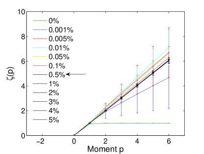
b)

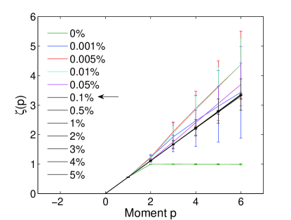
Figure 4: Plots showing the exponents $\zeta(p)$ against moment order $p$ of the generalized structure functions for various values of the percentage of large events excluded for (a) $\alpha=1.0$ and (b) $\alpha=1.8$. The arrows indicate the percentage beyond which convergence to the expected behaviour $\zeta(p)=p/\alpha$ is established. Both plots are for a sample size of $N=10^{6}$.

a)

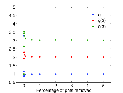
b)

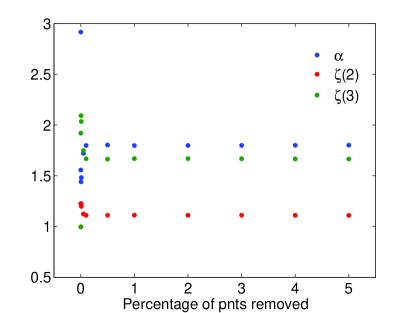
Figure 5: Plots showing the rapid convergence of the Lévy parameter $\alpha$; and the exponents of the $2^{nd}$ and $3^{rd}$ moments $\zeta(2)$ and $\zeta(3)$. The plots in (a) are for $\alpha=1.0$ and in (b) for $\alpha=1.8$ – both have $N=10^{6}.$ $\zeta(2)$ and $\zeta(3)$ are the best fit gradients of the $S^{p}$ vs. $\tau$ plots, and $\alpha$ is obtained from the inverse of the gradient of the $\zeta(p)$ vs. $p$ plot shown in Figure 4.

In Figure 4 we see that if no outliers are removed from the integral for $S^{p}$, the resulting values of $\zeta(p)$ for $p>\alpha$ saturate to unity. Removing a small fraction ($\sim$0.001%) of the outliers results in a drastic change in the $\zeta(p)$, again emphasising the strong effect these points have in the integral for $S^{p}$. The $\zeta(p)$ converge to the values predicted by (29) quite rapidly with $m/N$. The rate of convergence is illustrated in Figure 5 for the two cases shown in Figure 4. Convergence is achieved at $m/N=0.001$ for $\alpha=1.8$ and $m/N=0.005$ for $\alpha=1.0$; which correspond to the largest event being $y^{*}\simeq 18$ and $y^{*}\simeq 130$ respectively. These values lie in the region given by (16), as the asymptotic tail region of the PDF is valid for $y\gg\tau^{1/\alpha}=1$ here.

It is also instructive to investigate the effects of variations in sample size $N$ on the rates of convergence. Figure 6 illustrates these effects in the form of $\zeta(p)$ vs. $p$ plots for sizes $N=10^{5}$ and $N=5\times 10^{6}$ for a Lévy process of index $\alpha=1.0$. Recall that decreasing the sample size would result in further undersampling and thus poor statistics in the tails of the PDF. This can be clearly seen in Figure 6 (a) where we see a slow convergence to the line $\zeta(p)=p/\alpha$ which is achieved after $\sim 4$% of the data is excluded. The converse of this is shown in Figure 6 (b) where increasing the sample size by a factor of $20$ results in a very rapid convergence to scaling which is reached after only $\sim 0.5$% of the data is excluded.

a)

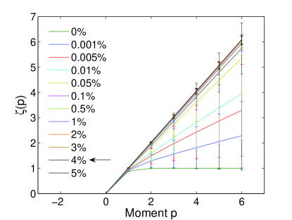
b)

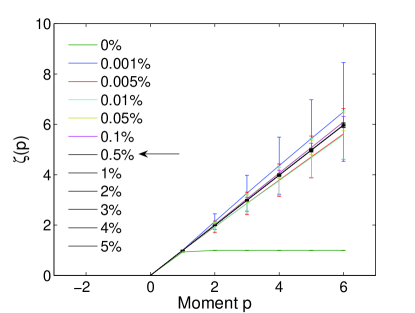
Figure 6: $\zeta(p)$ vs. $p$ plots for $\alpha=1.0$; (a) $N=10^{5}$ and (b) $N=5\times 10^{6}$.

Lastly we consider the behaviour of the outliers that are removed by this procedure. As we succesively remove more outliers (increasing $m$), the behaviour of $y_{m}^{*}$ will more closely correspond to that of $\bar{y}_{m}^{*}$. This is shown in Figure 7 where we plot $y_{m}^{*}(\tau)$ for increasing $m/N$. The anticipated scaling (25) appears at a value of $m/N$ corresponding to a few percent. A more established method for determining the scaling of outliers is a rank order (or Zipf) plot (see Sornette Sornette (2000)); this is shown in Figure 8 where we plot $y_{m}^{*}(m/N)$ for succesively large values of $\tau$. The scaling with $m/N$ is again as expected from (20)–(24), and the rank order plots also highlight scatter of individual realisations of $y_{m}^{*}$ from the ensemble average. In Figure 8 this becomes apparent at higher values of $\tau$. As we increase $\tau$ we require a higher fraction of points to be excluded before we regain the expected scaling with $m/N$. This breakdown of the scaling at higher values of $\tau$ follows from equations (30) and (31). We can see that $\Lambda$ increases with $\tau$ and so the distribution becomes more broad. Consequently this will require a higher fraction $m/N$ of points to be excluded so that we may regain the scaling behaviour (20). At the largest $\tau$, Figures 7 and 8 show a saturation indicative of the difference $y_{m}^{*}$ being dominated by a single extremal value $x$ of the original timeseries in (1). These plots are also a useful indicator of how feasable, for a dataset of size $N$, it would be to distinguish a departure from Lévy scaling in the tails.

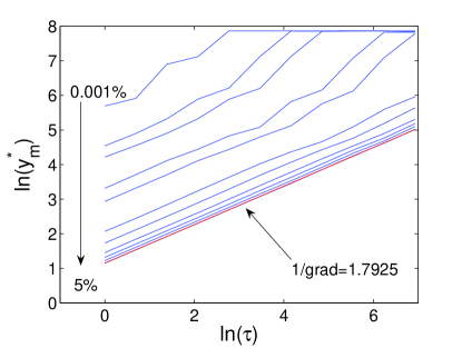
Figure 7: Log-log plot illustrating the scaling of the $m^{th}$ largest event $y_{m}^{*}$ with $\tau$ as $m$ is increased; $\alpha=1.8$ , $N=10^{6}$. For comparison with previous figures we indicate the % of points that would be excluded for the particular $m$.

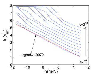
Figure 8: Log-log plot illustrating the scaling of the largest event $y_{m}^{*}$ with $m/N$ for various values of $\tau$; $\alpha=1.8$ , $N=10^{6}$.

IV summary and conclusions

In this paper we have presented a novel technique for ‘conditioning’ data to deal with anomalous scaling properties that arise due to finite size effects. We have demonstrated our ideas on a numerically generated symmetric $\alpha$-stable Lévy process. We are concerned with the situation of observations of natural systems, or of experiments, where the underlying PDF is not known a priori and where one inevitably has a finite length series of data. Hence we have proposed a technique that does not require a priori knowledge of the underlying process and that has consistency checks.

We have shown that ‘conditioning’ the data by progressively excluding the outliers, or extremal points, when computing the scaling exponents from the structure functions, recovers the underlying scaling of a self-affine process up to large order. For large datasets of a Lévy process this corresponds to removing 0.1-1% of the data. The conditioned structure functions then provide a straightforward method for determining the self-affine scaling exponent, in this case the Lévy index $\alpha$, directly from the slope of a plot of the exponents versus moment order.

This method offers two consistency checks. The first of these is that for a self-affine process, as we progressively remove more outliers we expect that the exponents obtained from the structure functions should converge on values which then do not vary. Practically speaking, one would plot the exponents as a function of the location of the last outlier excluded and expect a plateau that extended deep into the tail of the PDF. A second check is obtained by examining the scaling properties of these discarded outliers.

Importantly, the above analysis assumes that we have some relatively good statistics – in practice the high variability of the Lévy process due to the fat tails will always result in some lone extreme points with a finite probability of occurence, resulting in anomalous scaling exponents. This implies that we always need some way of cleaning or conditioning the data to recover the scaling behaviour. These lone points can have a drastic effect since in a Lévy-like process the largest value of a set of increments of a timeseries can be of the order of the total sum Bardou et al. (2002); Sornette (2000). Coupled with this we have that the tails of a distribution are described by the higher order moments (structure functions here). If the statistics of the tail are not well resolved then these moments will also give anomalous values of $\zeta(p)$.

In principle, this approach may be extended to the case of multi-affine timeseries and this will be the subject of further work.