Nonlinear magnetoacoustic waves in a cold plasma

Abstract

The equations describing planar magnetoacoustic waves of permanent form in a cold plasma are rewritten so as to highlight the presence of a naturally small parameter equal to the ratio of the electron and ion masses. If the magnetic field is not nearly perpendicular to the direction of wave propagation, this allows us to use a multiple-scale expansion to demonstrate the existence and nature of nonlinear wave solutions. Such solutions are found to have a rapid oscillation of constant amplitude superimposed on the underlying large-scale variation. The approximate equations for the large-scale variation are obtained by making an adiabatic approximation and in one limit, new explicit solitary pulse solutions are found. In the case of a perpendicular magnetic field, conditions for the existence of solitary pulses are derived. Our results are consistent with earlier studies which were restricted to waves having a velocity close to that of long-wavelength linear magnetoacoustic waves.

1 Introduction

For a plasma composed of cold electrons and a single species of cold ions, both collisions and Landau damping can be neglected with the result that a two-fluid model provides an accurate description (Kakutani et al. 1968). Such a model is governed by the continuity and momentum equations for electrons and ions, and Maxwell’s equations. In the study of non-relativistic hydromagnetic waves with a frequency much less than the plasma frequency, these equations may be simplified somewhat by neglecting the displacement current and taking the number densities of electrons and ions to be equal, except in Poisson’s equation (Kakutani et al. 1967). Then taking all quantities to be independent of $y$ and $z$ one arrives at a set of equations governing planar hydromagnetic waves. Il’ichev (1996) integrates these to obtain the following equations for a magnetoacoustic wave of permanent form propagating in the $x$-direction at a constant speed $V$: d vd ξ&=-RicosθVnw-R_iB_z,
d wd ξ=RicosθVnv+R_i^B_y+R_isinθ (1-n),
d ^Byd ξ=R_enw+RecosθVnB_z,
d Bzd ξ=-R_env-RecosθVn^B_y, where $\xi=x-Vt$,

$$\frac{1}{n}=1-\frac{1}{2V^{2}}\left(\hat{B}_{y}^{2}+2\hat{B}_{y}\sin\theta+B_{z}^{2}\right),$$ (1)

$$\hat{B}_{y}=B_{y}-\sin\theta,$$ (2)

and $\theta$ is the angle between the equilibrium magnetic field and the $x$-axis. In the above, $\xi$, the ion density $n$, the $y$ and $z$ components of the ion drift velocity $v$ and $w$, and the magnetic field $(B_{x},B_{y},B_{z})$ are normalized, respectively, by the characteristic length $l$, the equilibrium ion density, the Alfvén velocity $V_{A}$, and the equilibrium magnetic field strength. In such units the speed of a linear long-wavelength magnetoacoustic wave is unity. The remaining parameters are defined by $R_{i}=\omega_{ci}l/V_{A}$ and $R_{e}=\omega_{ce}l/V_{A}$ where $\omega_{ci}$ and $\omega_{ce}$ are the ion and electron cyclotron frequencies, respectively. The values of the dependent variables in the absence of a wave are zero for $v$, $w$, $\hat{B}_{y}$, and $B_{z}$, and unity in the case of $n$.

The results we present here originate from our observation that equations (1) may be rewritten so as to include a small parameter, $\varepsilon$. After introducing the variable $s\equiv R_{e}\xi/\bar{V}$, where $\bar{V}=V\sec\theta$, the equations take the form d vd s&=-ε{nw+¯VB_z},
d wd s=ε{nv+¯V^B_y+Vtanθ (1-n)},
d ^Byd s=n{¯Vw+B_z},
d Bzd s=-n{¯Vv+^B_y}, where $\varepsilon\equiv R_{i}/R_{e}$ is simply the ratio of the electron and ion masses. With $\varepsilon\sim 10^{-3}$ or smaller, any analytical treatment should make use of the smallness of this parameter and some form of perturbation theory is obviously called for. Furthermore, even a purely numerical method of solution should attempt to take advantage of the smallness of $\varepsilon$ as otherwise it means integrating over many small-scale variations before the underlying variation on the large scale takes place.

From (1) it can be seen that generally $v$ and $w$ change on a much slower scale than $\hat{B}_{y}$ and $B_{z}$. It is therefore natural to make an adiabatic approximation (see Haken (1983)) which is equivalent to equating the right-hand sides of (1) and (1) to zero. This gives

$$B_{z}=-\bar{V}w,\qquad\hat{B}_{y}=-\bar{V}v.$$ (3)

These relationships can be used to eliminate $\hat{B}_{y}$ and $B_{z}$ and it is shown in Appendix A that all the dependent variables can be expressed in terms of a single variable which itself satisfies a Newtonian type energy equation with a polynomial Sagdeev potential. This equation is then used to show the existence of solitary pulses and nonlinear waves on the larger scale. However, it should be stressed that the very nature of the adiabatic approximation as used in the above is to eliminate any variation on the smaller scale. Furthermore, the class of solutions to (1) is restricted, in view of relationships (3), which implies that at some particular value of $s$ the corresponding values of $(B_{z},w)$ and $(\hat{B}_{y},v)$ are not independent.

It is the purpose of this paper to construct a perturbation expansion based on the smallness of $\varepsilon$ which allows one to put the adiabatic approximation in context and to allow for rapid oscillations on the small scale. These effects have been studied analytically in Il’ichev (1996) and later numerically by Bakholdin and Il’ichev (1998) and Bakholdin et al. (2002). However, those studies were only carried out for the case $V=1+\mu/2$ where $\mu$ is small. In the present paper, the analytic theory based on the smallness of $\varepsilon$, a naturally small parameter, clearly shows the origin of all the basic features of the solutions they obtain and is not restricted to small $\mu$.

The underlying form of the governing equations suggests that a multiple-scale perturbation expansion is appropriate and this is carried out in Sec. 2 where explicit equations are obtained which describe the evolution of $v$, $w$, $\hat{B}_{y}$, and $B_{z}$ on both the small and large scale to lowest significant order in $\varepsilon$. This analysis is only valid when $\cos\theta$ is not small. For $\theta$ close to $\pm\pi/2$ singularities develop in (1) and so an alternative set of variables and equations derived from (1) must be employed, as is shown in Sec. 3. The final section summarizes our results and the further applicability of our approach is discussed.

2 Multiple-scale perturbation expansion

The perturbation expansion is based on the implication from equations (1) that two distinct spatial scales exist – a large one and a small one. We formally proceed by introducing multiple scales, $s,s_{1}=\varepsilon s,s_{2}=\varepsilon^{2}s,\ldots$ and treating them as independent variables so that

$$\frac{{\rm d}}{{\rm d}s}=\frac{\partial}{\partial s}+\varepsilon\frac{\partial}{\partial s_{1}}+\varepsilon^{2}\frac{\partial^{2}}{\partial s_{2}^{2}}+\ldots,$$

and allowing all dependent variables $f$ to be functions of $s,s_{1},\ldots$ and expressible in the form

$$f(s)=f_{0}(s,s_{1},\ldots)+\varepsilon f_{1}(s,s_{1},\dots)+\ldots,$$

although in the following it is not necessary to consider the scaled variables beyond $s$ (the small scale) and $s_{1}$ (the large scale). For a more general introduction to this form of perturbation theory see, for example, Nayfeh and Mook (1979) and Rowlands (1990).

Substituting the above form for the dependent variables into (1) and (1) gives to lowest order

$$\frac{\partial v_{0}}{\partial s}=0,\qquad\frac{\partial w_{0}}{\partial s}=0,$$

and so $v_{0}$ and $w_{0}$ can only be functions of $s_{1}$, and not $s$. At lowest order, (1) and (1) reduce to

$$\frac{\partial\hat{B}_{y0}}{\partial s}=n_{0}\{\bar{V}w_{0}+B_{z0}\},\qquad\frac{\partial B_{z0}}{\partial s}=n_{0}\{\bar{V}v_{0}+\hat{B}_{y0}\}.$$ (4)

Since $v_{0}$ and $w_{0}$ are independent of $s$, the solution of these equations is

$$\hat{B}_{y0}=h_{y}-\bar{V}v_{0},\qquad B_{z0}=h_{z}-\bar{V}w_{0},$$ (5)

where

$$\frac{\partial h_{y}}{\partial s}=n_{0}h_{z},\qquad\frac{\partial h_{z}}{\partial s}=-n_{0}h_{y}.$$

These equations have the solution

$$h_{y}=h(s_{1})\sin\phi,\qquad h_{z}=h(s_{1})\cos\phi,$$ (6)

where

$$\frac{\partial\phi}{\partial s}=n_{0}$$ (7)

and $h(s_{1})$ is an as yet to be determined function of $s_{1}$. Substituting the above results into (1) gives, to this approximation,

$$\frac{1}{n_{0}}=A+D(s_{1})\cos\phi+E(s_{1})\sin\phi$$ (8)

where

$$A=1+\frac{2V\tan\theta\;v_{0}-\bar{V}^{2}(w_{0}^{2}+v_{0}^{2})-h^{2}}{2V^{2}}$$ (9)

and

$$D=\frac{\bar{V}hw_{0}}{V^{2}},\qquad E=\frac{(\bar{V}v_{0}-\sin\theta)h}{V^{2}}.$$

Thus $A$, $D$, and $E$ are functions of $s_{1}$ only and the $s$ variation of $n_{0}$ is through $\phi$ only. Integrating the reciprocal of (7) after using (8) to express $n_{0}$ in terms of $\phi$ yields

$$A\phi+D\sin\phi-E\cos\phi=s-\tilde{s}(s_{1})$$ (10)

where $\tilde{s}$ is a function of $s_{1}$. A solution of (10) in the form $\phi=\phi(s,s_{1})$ is obtained in Appendix B.

We now proceed to next order and find using (1) that

$$\frac{\partial v_{1}}{\partial s}=-\frac{{\rm d}v_{0}}{{\rm d}s_{1}}-n_{0}w_{0}+\bar{V}^{2}w_{0}-\bar{V}h\cos\phi.\\$$ (11)

Since the right-hand side depends on $s$ via $\phi$ only, we replace $\partial v_{1}/\partial s$ by $n_{0}\partial v_{1}/\partial\phi$. Remembering that $v_{0}$, $w_{0}$ and $h$ are independent of $\phi$, and using (8), (11) is readily integrated to give

$$v_{1} = \left(\bar{V}^{2}w_{0}-\frac{{\rm d}v_{0}}{{\rm d}s_{1}}\right)(A\phi+D\sin\phi-E\cos\phi)-w_{0}\phi$$ (12)

$$\mbox{}+\bar{V}h\left(\frac{E}{4}\cos 2\phi-\frac{D}{4}(2\phi+\sin 2\phi)-A\sin\phi\right)+\tilde{v}(s_{1})$$

where $\tilde{v}(s_{1})$ is an undetermined function. To ensure that $v_{1}$ is a bounded function of $s$, we must remove terms proportional to $\phi$. After replacing $D$ by its definition this results in the consistency condition

$$A\frac{{\rm d}v_{0}}{{\rm d}s_{1}}=\left(A\bar{V}^{2}-1-\frac{\bar{V}^{2}h^{2}}{2V^{2}}\right)w_{0}.$$ (13)

This is the equation for the variation of $v_{0}$ on the slowly varying scale, $s_{1}$. Using (13) to simplify (12) leaves us with

$$v_{1}=\frac{1}{A}\left(w_{0}+\frac{\bar{V}hD}{2}\right)(D\sin\phi-E\cos\phi)+\bar{V}h\left(\frac{E}{4}\cos 2\phi-\frac{D}{4}\sin 2\phi-A\sin\phi\right)$$ (14)

in which $\tilde{v}$ has been absorbed into $v_{0}$.

Similarly, to first order, (1) yields

$$\frac{\partial w_{1}}{\partial s}=-\frac{{\rm d}w_{0}}{{\rm d}s_{1}}+n_{0}v_{0}-\bar{V}^{2}v_{0}+\bar{V}h\sin\phi+V\tan\theta\;(1-n_{0}).$$ (15)

After again replacing $\partial/\partial s$ by $n_{0}\partial/\partial\phi$ and integrating, to obtain a bounded $w_{1}$ we require that

$$A\frac{{\rm d}w_{0}}{{\rm d}s_{1}}=\left(1-A\bar{V}^{2}+\frac{\bar{V}^{2}h^{2}}{2V^{2}}\right)v_{0}+V\tan\theta\left(A-1-\frac{h^{2}}{2V^{2}}\right)$$ (16)

with the result that

$$w_{1} = \frac{1}{A}\left(V\tan\theta-v_{0}-\frac{\bar{V}hE}{2}\right)(D\sin\phi-E\cos\phi)$$ (17)

$$\mbox{}-\bar{V}h\left(A\cos\phi+\frac{D}{4}\cos 2\phi+\frac{E}{4}\sin 2\phi\right).$$

To lowest order, the adiabatic approximation (3) is

$$B_{z0}=-\bar{V}w_{0},\qquad\hat{B}_{y0}=-\bar{V}v_{0}.$$ (18)

Comparison with equations (5) shows that this approximation is equivalent to setting $h=0$. Equations (13) and (16) then form a complete set which can be integrated. The details are given in Appendix A. In particular, the existence of solitary pulses is proven.

If the adiabatic approximation is not made, it is necessary to obtain an equation for the variation of $h$ on the $s_{1}$ scale. This is achieved by considering the equations for $\hat{B}_{y}$ and $B_{z}$ to next order in $\varepsilon$. From (1) and (1) we may write, respectively,

$$\frac{\partial\hat{B}_{y1}}{\partial s}+\frac{\partial\hat{B}_{y0}}{\partial s_{1}} = n_{0}\{\bar{V}w_{1}+B_{z1}\}+n_{1}h\cos\phi,$$

$$\frac{\partial B_{z1}}{\partial s}+\frac{\partial B_{z0}}{\partial s_{1}} = -n_{0}\{\bar{V}v_{1}+\hat{B}_{y1}\}-n_{1}h\sin\phi.$$

Since the variation of all coefficients with $s$ is through $\phi$, we replace $\partial/\partial s$ by $n_{0}\partial/\partial\phi$ and rewrite the above equations as ∂^By1∂ϕ+1n0∂^By0∂s1&= ¯Vw_1+B_z1+n1hn0cosϕ,
∂Bz1∂ϕ+1n0∂Bz0∂s1= -¯Vv_1-^B_y1-n1hn0sinϕ. We proceed by adding (2) multiplied by $\sin\phi$ to (2) multiplied by $\cos\phi$ and then integrating from 0 to $2\pi$. Insisting that $\hat{B}_{y1}$ and $B_{z1}$ are periodic functions of $\phi$ means that

$$\left\langle\frac{\partial\hat{B}_{y1}}{\partial\phi}\sin\phi\right\rangle=-\left\langle\hat{B}_{y1}\cos\phi\right\rangle,\qquad\left\langle\frac{\partial B_{z1}}{\partial\phi}\cos\phi\right\rangle=\left\langle B_{z1}\sin\phi\right\rangle,$$

where $\left\langle\cdot\right\rangle$ denotes the average as $\phi$ varies from 0 to $2\pi$. The combined equations then reduce to the following equation for the variation of $h$:

$$\left\langle\frac{1}{n_{0}}\right\rangle\frac{{\rm d}h}{{\rm d}s_{1}}=\bar{V}\left\{\frac{{\rm d}v_{0}}{{\rm d}s_{1}}\left\langle\frac{\sin\phi}{n_{0}}\right\rangle+\frac{{\rm d}w_{0}}{{\rm d}s_{1}}\left\langle\frac{\cos\phi}{n_{0}}\right\rangle+\left\langle w_{1}\sin\phi\right\rangle-\left\langle v_{1}\cos\phi\right\rangle\right\}.$$ (19)

Using (8), (14), and (17) we have

$$\left\langle\frac{1}{n_{0}}\right\rangle=A,\qquad\left\langle\frac{\sin\phi}{n_{0}}\right\rangle=\frac{E}{2},\qquad\left\langle\frac{\cos\phi}{n_{0}}\right\rangle=\frac{D}{2},$$

$$\left\langle w_{1}\sin\phi\right\rangle=\left(V\tan\theta-v_{0}-\frac{\bar{V}hE}{2}\right)\frac{D}{2A},\qquad\left\langle v_{1}\cos\phi\right\rangle=-\left(1+\frac{\bar{V}^{2}h^{2}}{2V^{2}}\right)\frac{Ew_{0}}{2A}.$$

Then inserting the above expressions and results (13) and (16) into (19) and simplifying we find that the right-hand side of (19) is zero and hence that $h$ is a constant. This is in agreement with the result obtained for $V$ close to 1 in Il’ichev (1996).

In summary, we have seen that to lowest order, the ion drift velocity components $v$ and $w$ only show large-scale variation. Fast periodic variation occurs at the next order of approximation, as given by (14) and (17), but given the smallness of $\varepsilon$, these oscillations would be barely discernible. On the other hand, even to lowest order, the magnetic field components show rapid oscillations on top of the large-scale variation:

$$\hat{B}_{y0}=-\bar{V}v_{0}(s_{1})+h\sin\phi(s,s_{1}),\qquad B_{z0}=-\bar{V}w_{0}(s_{1})+h\cos\phi(s,s_{1}),$$

where, as is shown in Appendix B, $\sin\phi$ and $\cos\phi$ are periodic functions of the variable $S$ given by (40).

3 The small $\cos\theta$ and $\theta=\pm\pi/2$ limits

So far we have treated $\cos\theta$ as finite but our treatment does not allow one to pass to the case $\cos\theta=0$ since in this limit $\bar{V}$ becomes infinite. To consider this limit we write $\theta=\pm\pi/2\mp\sqrt{\varepsilon}\psi$ so that $\cos\theta=\sin(\sqrt{\varepsilon}\psi)\simeq\sqrt{\varepsilon}\psi$. (In the remainder of this section the upper and lower signs refer to the cases where $\theta$ is in the neighbourhood of $\pi/2$ and $-\pi/2$, respectively.) It is now necessary to go back to the original equations expressed in terms of $\xi$ rather than $s$ and define $X\equiv\sqrt{R_{i}R_{e}}\xi$. Also, to avoid singular solutions we need to use scaled versions of the ion drift velocities, defined by $\bar{v}=v/\sqrt{\varepsilon}$ and $\bar{w}=w/\sqrt{\varepsilon}$. Then dividing (1) by $\sqrt{R_{i}R_{e}}$ we obtain d ¯vd X&=-B_z+O(εψ),
d ¯wd X=^B_y±1-n+O(εψ^2),
d ^Byd X=n¯w+nBzVψ+O(εψ^3),
d Bzd X=-n¯v-n^ByVψ+O(εψ^3) with

$$\frac{1}{n}=1-\frac{1}{2V^{2}}\left(\hat{B}_{y}^{2}\pm 2\hat{B}_{y}+B_{z}^{2}\right)+O(\varepsilon\psi^{2}).$$ (20)

Any solution to the above equations will be such that $\bar{v}\sim B$ and hence the real velocity $v=\sqrt{\varepsilon}\bar{v}$ will be small compared to $B$.

For the $\theta=\pm\pi/2$ limits, equations (3) reduce to d ¯vd X=-B_z,   d Bzd X=-n¯v,
d ¯wd X=^B_y±1-n,   d ^Byd X=n¯w. We now define an operator $L$ by

$$Lf\equiv\frac{{\rm d}}{{\rm d}X}\left(\frac{1}{n}\frac{{\rm d}f}{{\rm d}X}\right).$$

Then from (3) and (3) it can be seen that, respectively, LB_z&=B_z,
LB_y=B_y-n, in which we have re-instated $B_{y}$, as given in (2). Combining equations (3) gives

$$B_{y}LB_{z}-B_{z}LB_{y}=B_{z}n.$$

Integrating this over one period (or all $X$ if boundary conditions permit) yields

$$\left\langle B_{z}n\right\rangle=0,$$ (21)

where $\left\langle\cdot\right\rangle$ denotes the integral over $X$. Similarly, (3) and (3) imply that

$$\left\langle B_{z}\right\rangle=0,\qquad\left\langle B_{y}\right\rangle=\left\langle n\right\rangle.$$ (22)

Relations (21) and (22) are satisfied if $n$ and $B_{y}$ are even functions and $B_{z}$ is an odd function of $X$.

We can demonstrate the existence of a non-trivial solution of (3) by taking $B_{z}=0$. In this case (20) becomes

$$\frac{1}{n}=\alpha(1-\beta B_{y}^{2})$$

where

$$\alpha=1+\frac{1}{2V^{2}},\qquad\beta=\frac{1}{1+2V^{2}},$$ (23)

with the result that (3) can be re-expressed as

$$\alpha\frac{{\rm d}}{{\rm d}X}\left((1-\beta B_{y}^{2})\frac{{\rm d}B_{y}}{{\rm d}X}\right)=B_{y}-\frac{1}{\alpha(1-\beta B_{y}^{2})}.$$

Letting $p={\rm d}B_{y}/{\rm d}X$, this can be written as the following first-order differential equation for $p^{2}$:

$$\frac{{\rm d}p^{2}}{{\rm d}B_{y}}-\left(\frac{4\beta B_{y}}{1-\beta B_{y}^{2}}\right)p^{2}=\frac{2}{\alpha}\left(\frac{B_{y}}{1-\beta B_{y}^{2}}-\frac{1}{\alpha(1-\beta B_{y}^{2})^{2}}\right)$$

which has an integrating factor of $(1-\beta B_{y}^{2})^{2}$. Hence the solution is given by

$$p^{2}=\frac{2Q}{\alpha(1-\beta B_{y}^{2})^{2}}$$ (24)

where

$$Q=\frac{B_{y}^{2}}{2}-\frac{\beta B_{y}^{4}}{4}-\frac{B_{y}}{\alpha}+Q_{0}$$ (25)

and $Q_{0}$ is an integration constant. For a solitary pulse solution, the appropriate boundary conditions are $B_{y}\to\pm 1$ and $Q\to 0$ as $|X|\to\infty$. Using these allows us to determine $Q_{0}$. We then rewrite (25) as the following expansion in $\hat{B}_{y}$:

$$Q=\hat{B}_{y}^{2}\left\{\frac{1-3\beta}{2}\mp\beta\hat{B}_{y}-\frac{\beta}{4}\hat{B}_{y}^{2}\right\}.$$ (26)

A necessary condition for the existence of solitary pulses is therefore that $\beta<1/3$. In addition, from (24) it can be seen that $p$ is singular at $B_{y}^{2}=1/\beta$. Hence, for a solitary pulse to exist, at least one of the two non-trivial zeros of the expression for $Q$ given in (26) must lie within the range $-1/\sqrt{\beta}\mp 1<\hat{B}_{y}<1/\sqrt{\beta}\mp 1$. The zero which is larger in magnitude never satisfies this. The remaining zero at $\pm\sqrt{2/\beta-2}\mp 2$ satisfies the condition if $\beta>1/9$. Using (23) we can now write the sufficient condition for the existence of a solitary pulse solution as $1<V^{2}<4$.

As a check on our calculation we look at the case when $V=1+\mu/2$ for small positive $\mu$. Then (24) reduces to

$$\left(\frac{{\rm d}\hat{B}_{y}}{{\rm d}X}\right)^{2}=\frac{\hat{B}_{y}^{2}}{4}(\hat{B}_{y}\pm 4)(\pm\mu-\hat{B}_{y})$$

to lowest order in $\mu$. The above equation has the solution

$$\hat{B}_{y}=\pm\mu\mathop{\mathrm{sech}}\nolimits^{2}\mbox{$\frac{1}{2}$}\sqrt{\mu}(X-X_{0})+O(\mu^{2})$$

where $X_{0}$ is an arbitrary constant. This is in agreement with the result given in Bakholdin and Il’ichev (1998).

4 Conclusions

We have studied a set of magnetohydrodynamic equations for planar magnetoacoustic waves of permanent form propagating in a two-component cold plasma and, by taking advantage of the smallness of the ratio of the electron to ion masses, have obtained a reduced set of equations which describe the large-scale variation of the magnetoacoustic wave solution of the full equations. Superimposed on the large-scale variation, multiple-scale perturbation analysis indicates that there is a rapid oscillation which is of constant amplitude in the case of the lowest-order magnetic field components. These results are consistent with the study of Il’ichev (1996) which was restricted to a narrow range of velocities. In addition, the approach expounded in this paper puts the adiabatic approximation into its true context.

In this work we have obtained various conditions for the existence of solitary pulses. Whether these solutions correspond to phenomena that could occur in nature depends on whether they are stable. Linear stability analysis of the solutions shown to exist in this paper is a challenging problem. However, the numerical solution of the full (time-dependent) system of equations obtained by Bakholdin and Il’ichev (1998), show that for a range of initial conditions the solution relaxes to the type of solution shown to exist here. This suggests that our solutions are stable, at least to perturbations applied in the direction of propagation.

Although the equations studied here arise from a magnetohydrodynamics problem, the method is applicable to a more general set of nonlinear equations where two distinct scales are a basic feature. An advantage of the present study is that the equations obtained on the large scale can be investigated analytically and describe real physical processes. Although we have only looked at cold plasmas, an exactly analogous procedure can be applied to the case of warm plasmas, at the expense of some additional algebraic complexity. The relevant governing equations are given in Bakholdin et al. (2002).

Appendix A Adiabatic approximation

When $h=0$, the coupled equations for $v_{0}$ and $w_{0}$, namely (13) and (16), reduce to

$$\frac{{\rm d}v_{0}}{{\rm d}s_{1}}=\left(\bar{V}^{2}-\frac{1}{A}\right)w_{0}$$ (27)

and

$$\frac{{\rm d}w_{0}}{{\rm d}s_{1}}=\left(\frac{1}{A}-\bar{V}^{2}\right)v_{0}+V\tan\theta\;\left(1-\frac{1}{A}\right).$$ (28)

Multiplying (27) and (28) by $2v_{0}$ and $2w_{0}$, respectively, and adding gives

$$\frac{{\rm d}}{{\rm d}s_{1}}(v_{0}^{2}+w_{0}^{2})=2V\tan\theta\;\left(1-\frac{1}{A}\right)w_{0}.$$ (29)

Differentiating (9) with respect to $s_{1}$ and using the above, one obtains

$$\frac{{\rm d}A}{{\rm d}s_{1}}=\frac{(\bar{V}^{2}-1)\tan\theta}{V}\frac{w_{0}}{A},$$

or, provided that $\bar{V}^{2}\neq 1$,

$$w_{0}=\frac{A}{\kappa}\frac{{\rm d}A}{{\rm d}s_{1}},\qquad\kappa=\frac{(\bar{V}^{2}-1)\tan\theta}{V}.$$ (30)

Substituting (30) into (29) and (27) and integrating yields, respectively,

$$v_{0}^{2}+w_{0}^{2}=C_{1}+V\kappa^{-1}\tan\theta(A^{2}-2A)$$ (31)

and

$$v_{0}=C_{2}+\kappa^{-1}(\mbox{$\frac{1}{2}$}\bar{V}^{2}A^{2}-A)$$ (32)

where $C_{1}$ and $C_{2}$ are integration constants. Finally, after combining (30), (31) and (32) one obtains

$$\left(A\frac{{\rm d}A}{{\rm d}s_{1}}\right)^{2}=\sum_{m=0}^{4}\gamma_{m}A^{m}$$ (33)

in which

$$\gamma_{0}=(C_{1}-C_{2}^{2})\kappa^{2},\quad\gamma_{1}=2(C_{2}-V\tan\theta)\kappa,\quad\gamma_{2}=(V\tan\theta-C_{2}\bar{V}^{2})\kappa-1,$$

$$\gamma_{3}=\bar{V}^{2},\qquad\gamma_{4}=-\mbox{$\frac{1}{4}$}\bar{V}^{4}.$$

This is of the form of the energy equation of a particle with position $A$ in a Sagdeev potential which is minus the right-hand side of (33). In general, nonlinear waves exist and in particular solitary pulses. The latter can occur when the boundary conditions are such that $v\to 0$, $w\to 0$, and $n\to 1$ as $s_{1}\to\pm\infty$. Using the result that in this limit $A\to 1$, the boundary conditions allow us to use (31) and (32) to determine the integration constants in this case:

$$C_{1}=V\kappa^{-1}\tan\theta,\qquad C_{2}=(1-\mbox{$\frac{1}{2}$}\bar{V}^{2})\kappa^{-1}.$$

Then (33) reduces to

$$\left(A\frac{{\rm d}A}{{\rm d}s_{1}}\right)^{2}=\frac{(A-1)^{2}}{4}(a+bA+cA^{2})$$ (34)

where

$$a=4(\bar{V}^{2}-1)\tan^{2}\theta-(\bar{V}^{2}-2)^{2},\qquad b=2\bar{V}^{2}(2-\bar{V}^{2}),\qquad c=-\bar{V}^{4}.$$

The requirement that (34) gives rise to a solitary pulse is that $a+b+c>0$. Using the above renders this condition as $(\bar{V}^{2}-1)(1-V^{2})>0$ which on rearranging yields

$$\cos^{2}\theta<V^{2}<1.$$

As illustrated in Fig. 1, since $c<0$, if the above condition is satisfied, compressive solitary pulses will always occur. However, rarefactive pulses are only possible if the smaller root of $a+bA+cA^{2}=0$ is above zero. This will occur if $a<0$ and $\bar{V}^{2}<2$. These requirements are equivalent to the condition

$$V^{2}<2(1-|\sin\theta\,|).$$

This implies that if the values of $V$ and $\theta$ are such that compressive pulses exist, then rarefactive pulses will also occur if $|\theta|\leqslant\pi/6$.

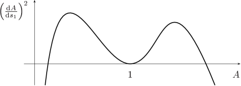
Figure 1: Phase plane for (34) when conditions are such that both compressive and rarefactive solitary pulses occur.

It is possible to integrate (34) to obtain the spatial variation of the solitary pulses implicitly. An approximate explicit solution can be obtained when $\bar{V}^{2}$ is just above 1. Introducing $U\equiv A-1$, (34) becomes

$$\left(\frac{{\rm d}U}{{\rm d}s_{1}}\right)^{2}=\frac{\bar{V}^{4}U^{2}(U_{+}-U)(U-U_{-})}{(1+U)^{2}}$$ (35)

where

$$U_{\pm}=\frac{2\sqrt{\bar{V}^{2}-1}}{\bar{V}^{2}}\left(\pm\tan\theta-\sqrt{\bar{V}^{2}-1}\right).$$

If $\sqrt{\bar{V}^{2}-1}\!<\!\!<\!|\tan\theta\,|$, then $U_{\pm}\simeq\pm\nu$ where

$$\nu=\frac{2\sqrt{\bar{V}^{2}-1}\tan\theta}{\bar{V}^{2}}.$$

For solitary pulse solutions, $|U|<|U_{\pm}|$, and so if $\tan\theta$ is of order unity, $U\!<\!\!<\!1$. Hence (35) reduces to

$$\frac{{\rm d}U}{{\rm d}s_{1}}=U\sqrt{\nu^{2}-U^{2}}$$

at lowest order and one obtains

$$A\simeq 1\pm\nu\mathop{\mathrm{sech}}\nolimits\nu s_{1}.$$ (36)

Using (30) and (32) we can then obtain the corresponding expressions for $w_{0}$ and $v_{0}$:

$$w_{0}\simeq\mp 4V\tan\theta\mathop{\mathrm{sech}}\nolimits\nu s_{1}\tanh\nu s_{1},\qquad v_{0}\simeq 2V\tan\theta\mathop{\mathrm{sech}}\nolimits^{2}\nu s_{1}.$$ (37)

In this adiabatic approximation, the lowest order components of the magnetic field are just multiples of these quantities, as given by (18).

We can now also use (36) and (37) to obtain the solution when $\bar{V}^{2}=1$. This corresponds to the limit $\nu\to 0$ in which case $A\to 1$, $w_{0}\to 0$, and $v_{0}\to 2V\tan\theta$. As a check on our calculation, we note that these results are consistent with the definition of $A$ as given by (9) when $h=0$.

Appendix B Explicit expression for $\phi(s,s_{1})$

The variation of $\phi$ with $s$ is given implicitly by (10). An explicit expression can be obtained by writing the equation in the form

$$S+\psi=\phi+\psi-\sigma\sin(\phi+\psi)$$ (38)

where $S=(s-\tilde{s})/A$, $\psi=\arg(-D+{\rm i}E)$ and $\sigma=\sqrt{D^{2}+E^{2}}/A$. The following explicit solution to (38) was first obtained by Jackson (1960) (although for a more transparent exposition see p.154 of Infeld and Rowlands (2000)):

$$\phi=S+2\sum_{m=1}^{\infty}\frac{J_{m}(m\sigma)}{m}\sin m(S+\psi).$$ (39)

It can be seen that $\phi$ has a directed component, $S$, on which a periodic variation is superimposed. Since $A$ and hence the period vary on the $s_{1}$ timescale, to the order in $\varepsilon$ to which (39) applies, it is more appropriate to re-define $S$ by

$$S=\int_{\tilde{s}}^{s}\frac{{\rm d}s^{\prime}}{A(\varepsilon s^{\prime})}.$$ (40)

Such a definition avoids secular terms at higher order in the $\varepsilon$ expansion.

References

- Bakholdin and Il’ichev (1998) Bakholdin, I. and Il’ichev, A. 1998 J. Plasma Phys. 60, 569.
- Bakholdin et al. (2002) Bakholdin, I., Il’ichev, A. and Zharkov, A. 2002 J. Plasma Phys. 67, 1.
- Haken (1983) Haken, H. 1983 Synergetics. 3rd edn. Springer-Verlag, Berlin.
- Il’ichev (1996) Il’ichev, A. 1996 J. Plasma Phys. 55, 181.
- Infeld and Rowlands (2000) Infeld, E. and Rowlands, G. 2000 Nonlinear Waves, Solitons and Chaos. 2nd edn. Cambridge: Cambridge University Press.
- Jackson (1960) Jackson, E. A. 1960 Phys. Fluids 3, 831.
- Kakutani et al. (1967) Kakutani, T., Kawahara, T. and Taniuti, T. 1967 J. Phys. Soc. Japan 23, 1138.
- Kakutani et al. (1968) Kakutani, T., Ono, H., Taniuti, T. and Wei, C.-C. 1968 J. Phys. Soc. Japan 24, 1159.
- Nayfeh and Mook (1979) Nayfeh, A. H. and Mook, D. T. 1979 Nonlinear Oscillations. Wiley, New York.
- Rowlands (1990) Rowlands, G. 1990 Non-Linear Phenomena in Science and Engineering. Ellis Horwood, London.