Calculation of material properties and ray tracing in transformation media

Abstract

Complex and interesting electromagnetic behavior can be found in spaces with non-flat topology. When considering the properties of an electromagnetic medium under an arbitrary coordinate transformation an alternative interpretation presents itself. The transformed material property tensors may be interpreted as a different set of material properties in a flat, Cartesian space. We describe the calculation of these material properties for coordinate transformations that describe spaces with spherical or cylindrical holes in them. The resulting material properties can then implement invisibility cloaks in flat space. We also describe a method for performing geometric ray tracing in these materials which are both inhomogeneous and anisotropic in their electric permittivity and magnetic permeability.

I
Introduction

Recently the use of coordinate transformations to produce material specifications that control electromagnetic fields in interesting and useful ways has been discussed. We have described such a method in which the transformation properties of Maxwell’s equations and the constitutive relations can yield material descriptions that implement surprising functionality, such as invisibilityPendry et al. (2006). Another author described a similar method where the two dimensional Helmholtz equation is transformed to produce similar effects in the geometric limitLeonhardt (2006). We note that these theoretical design methods are of more than academic interest, as the material specifications can be implemented with metamaterial technologySmith et al. (2004); Cubukcu et al. (2003a, b); Yen et al. (2004); Linden et al. (2004); Schurig et al. (2006). There has also been recent work on invisibility cloaking that does not employ the transformation methodAlu and Engheta (2005); Milton and Nicorovici (2006).

In this article we describe how to calculate these material properties directly as Cartesian tensors and to perform ray tracing on devices composed of these materials. We work out two examples in detail, the spherical and cylindrical invisibility cloak.

II Material Properties

We will describe the transformation properties of the electromagnetic, material property tensors. We first note that the Minkowski form of Maxwell’s equationsE.J.Post (1962); Jackson (1975); Kong (1990)

$$F_{\alpha\beta,\mu}+F_{\beta\mu,\alpha}+F_{\mu\alpha,\beta} =0$$ (1a)

$$G_{,\alpha}^{\alpha\beta} =J^{\beta}$$ (1b)

is form invariant for general space-time transformations. $$F_{\alpha\beta} G^{\alpha\beta} J^{\beta}$$ is the tensor of electric field and magnetic induction, and is the tensor density of electric displacement and magnetic field, and  is the source vecto. In SI units the components are

$$\left(F_{\alpha\beta}\right) =\left(\begin{array}[c]{cccc}0&-E_{1}&-E_{2}&-E_{3}\\ E_{1}&0&B_{3}&-B_{2}\\ E_{2}&-B_{3}&0&B_{1}\\ E_{3}&B_{2}&-B_{1}&0\end{array}\right)$$ (2e)

$$\left(G^{\alpha\beta}\right) =\left(\begin{array}[c]{cccc}0&-D_{1}&-D_{2}&-D_{3}\\ D_{1}&0&H_{3}&-H_{2}\\ D_{2}&-H_{3}&0&H_{1}\\ D_{3}&H_{2}&-H_{1}&0\end{array}\right)$$ (2j)

$$\left(J^{\beta}\right) =\left(\begin{array}[c]{c}\rho\\ J_{1}\\ J_{2}\\ J_{3}\end{array}\right)$$ (2o)

All of the information regarding the topology of the space is contained in the constitutive relations

$$G^{\alpha\beta}=\frac{1}{2}C^{\alpha\beta\mu\nu}F_{\mu\nu}$$ (3)

where $C^{\alpha\beta\mu\nu}$ is the constitutive tensor representing the properties of the medium, including its permittivity, permeability and bianisotropic properties. $C^{\alpha\beta\mu\nu}$ is a tensor density of weight +1, so it transforms asE.J.Post (1962)

$$C^{\alpha^{\prime}\beta^{\prime}\mu^{\prime}\nu^{\prime}}=\left|\det\left(\Lambda_{\;\alpha}^{\alpha^{\prime}}\right)\right|^{-1}\Lambda_{\;\alpha}^{\alpha^{\prime}}\Lambda_{\;\beta}^{\beta^{\prime}}\Lambda_{\;\mu}^{\mu^{\prime}}\Lambda_{\;\nu}^{\nu^{\prime}}C^{\alpha\beta\mu\nu}$$ (4)

written in terms of the Jacobian transformation matrix

$$\Lambda_{\;\alpha}^{\alpha^{\prime}}=\frac{\partial x^{\alpha^{\prime}}}{\partial x^{\alpha}}$$ (5)

which is just the derivative of the transformed coordinates with respect to the original coordinates. If we restrict ourselves to transformations that are time invariant, the permittivity and permeability are also tensors individually. Specifically, they are tensor densities of weight +1, which transform asShyroki (2006); E.J.Post (1962)

$$\varepsilon^{i^{\prime}j^{\prime}} =\left|\det\left(\Lambda_{\;i}^{i^{\prime}}\right)\right|^{-1}\Lambda_{\;i}^{i^{\prime}}\Lambda_{\;j}^{j^{\prime}}\varepsilon^{ij}$$ (6a)

$$\mu^{i^{\prime}j^{\prime}} =\left|\det\left(\Lambda_{\;i}^{i^{\prime}}\right)\right|^{-1}\Lambda_{\;i}^{i^{\prime}}\Lambda_{\;j}^{j^{\prime}}\mu^{ij}$$ (6b)

where the roman indices run from 1 to 3, for the three spatial coordinates, as is standard practice. Equations (6) are the primary tools for the transformation design method when the base medium is not bianisotropic and the desired device moves or change shape with speeds much less than that of light, i.e. probably all devices of practical interest. These equations can be shown to be exactly equivalent to the results derived by Ward and PendryWard and Pendry (1996).

If the original medium is isotropic, (6) can also be written in terms of the metricShyroki (2006); Leonhardt and Philbin (2006)

$$\varepsilon^{i^{\prime}j^{\prime}} =\left|\det\left(g^{i^{\prime}j^{\prime}}\right)\right|^{-1/2}g^{i^{\prime}j^{\prime}}\varepsilon$$ (7)

$$\mu^{i^{\prime}j^{\prime}} =\left|\det\left(g^{i^{\prime}j^{\prime}}\right)\right|^{-1/2}g^{i^{\prime}j^{\prime}}\mu$$ (8)

where the metric is given by

$$g^{i^{\prime}j^{\prime}}=\Lambda_{\;k}^{i^{\prime}}\Lambda_{\;l}^{j^{\prime}}\delta^{kl}$$ (9)

Maxwell’s equations, (1), together with the medium specified by (4) or (6) describe a single electromagnetic behavior, but this behavior can be interpreted in two ways.

One way, the traditional way, is that the material property tensors that appear on the left and right hand sides of (4) or (6) represent the same material properties, but in different spaces. The components in the transformed space are different form those in the original space, due to the topology of the transformation. We will refer to this view as the topological interpretation.

An alternative interpretation, is that the material property tensors on the left and right hand sides of (4) or (6) represent different material properties. Both sets of tensor components are interpreted as components in a flat, Cartesian space. The form invariance of Maxwell’s equations insures that both interpretations lead to the same electromagnetic behavior. We will refer to this view as the materials interpretation.

To design something of interest, one imagines a space with some desired property, a hole for example. Then one constructs the coordinate transformation of the space with this desired property. Using (4) or (6) one can then calculate a set of material properties that will implement this interesting property of the imagined space in our own boring, flat, Cartesian space.

II.1 Spherical Cloak

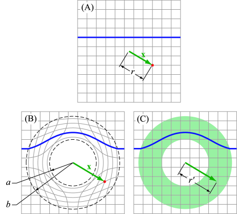
Figure 1: The thick blue line shows the path of the same ray in (A) the original Cartesian space, and under two different interpretations of the electromagnetic equations, (B) the topological interpretation and (C) the materials interpretation. The position vector $\mathbf{x}$ is shown in both the original and transformed spaces, and the length of the vector where the transformed components are interpreted as Cartesian components is shown in (C).

The spherical cloak is designed by considering a spherically symmetric coordinate transformation. This transformation compresses all the space in a volume of radius, $b$, into a spherical shell of inner radius, $a$, and outer radius, $b$. Consider a position vector, $\mathbf{x}$. In the original coordinate system (Fig.1A) it has components, $x^{i}$, and in the transformed coordinate system (Fig.1B), $x^{i^{\prime}}$. Of course, its magnitude, $r$, is independent of coordinate system

$$r=\left(x^{i}x^{j}\delta_{ij}\right)^{1/2}=\left(x^{i^{\prime}}x^{j^{\prime}}g_{i^{\prime}j^{\prime}}\right)^{1/2}$$ (10)

where $g_{i^{\prime}j^{\prime}}$ is the metric of the transformed space. In the materials interpretation, (Fig.1C), we consider the components, $x^{i^{\prime}}$, to be the components of a Cartesian vector, and its magnitude is found using the appropriate flat space metric

$$r^{\prime}=\left(x^{i^{\prime}}x^{j^{\prime}}\delta_{i^{\prime}j^{\prime}}\right)^{1/2}$$ (11)

Perhaps the simplest spherical cloak transformation maps points from a radius, $r$, to a radius, $r^{\prime}$, according to the following linear function

$$r^{\prime}=\frac{b-a}{b}r+a$$ (12)

which we apply over the domain, $0\leq r\leq b$, (or equivalently, $a\leq r^{\prime}\leq b$). Outside this domain we assume an identity transformation. (All equations in the remainder of this article apply only to the transformation domain.) We must always limit the transformation to apply only over a finite region of space if we wish to implement it with materials of finite extent. Note that when $r=0$ then $r^{\prime}=a$, so that the origin is mapped out to a finite radius, opening up a whole in space. Note also that when $r=b$ then $r^{\prime}=b$, so that space at the outer boundary of the transformation is undistorted and there is no discontinuity with the space outside the transformation domain.

Now since our transformation is radially symmetric, the unit vectors in materials interpretation and in the original space must be equal.

$$\frac{x^{i^{\prime}}}{r^{\prime}}=\frac{x^{i}}{r}\delta_{\;i}^{i^{\prime}}$$ (13)

Expressing the components of the position vector in the transformed space in terms of only the components in the original space, using (12), we obtain.

$$x^{i^{\prime}}=\frac{b-a}{b}x^{i}\delta_{\;i}^{i^{\prime}}+a\frac{x^{i}}{r}\delta_{\;i}^{i^{\prime}}$$ (14)

Now that we have this expression, we need not worry about the interpretations of transformed space, we can just proceed in standard fashion to compute the transformation matrix. To take the derivative of this expression we note that

$$\frac{\partial}{\partial x^{j}}\frac{x^{i}}{r}=-\frac{x^{i}x^{k}\delta_{kj}}{r^{3}}+\frac{1}{r}\delta_{\;j}^{i}$$ (15)

and obtain the transformation matrix

$$\Lambda_{\;j}^{i^{\prime}}=\frac{r^{\prime}}{r}\delta_{\;j}^{i^{\prime}}-\frac{ax^{i}x^{k}\delta_{\;i}^{i^{\prime}}\delta_{kj}}{r^{3}}$$ (16)

The components of this expression written out are

$$\left(\Lambda_{\;j}^{i^{\prime}}\right)=\left(\begin{array}[c]{ccc}\frac{r^{\prime}}{r}-\frac{ax^{2}}{r^{3}}&-\frac{axy}{r^{3}}&-\frac{axz}{r^{3}}\\ -\frac{ayx}{r^{3}}&\frac{r^{\prime}}{r}-\frac{ay^{2}}{r^{3}}&-\frac{ayz}{r^{3}}\\ -\frac{azx}{r^{3}}&-\frac{azy}{r^{3}}&\frac{r^{\prime}}{r}-\frac{az^{2}}{r^{3}}\end{array}\right)$$ (17)

To calculate the determinant of this matrix we note that we can always rotate into a coordinate system such that

$$\left(x^{i}\right)=(r,0,0)$$ (18)

then the determinant is, by inspection, given by

$$\det(\Lambda_{\;j}^{i^{\prime}})=\frac{r^{\prime}-a}{r}\left(\frac{r^{\prime}}{r}\right)^{2}$$ (19)

If we assume that our original medium is free space, then the permittivity and permeability will be equal to each other. As a short hand, we define a tensor, $n^{i^{\prime}j^{\prime}}$, to represent both.

$$n^{i^{\prime}j^{\prime}}\equiv\varepsilon^{i^{\prime}j^{\prime}}=\mu^{i^{\prime}j^{\prime}}$$ (20)

Though this definition is suggestive of refractive index, $n^{i^{\prime}j^{\prime}}$ would only represent the scalar refractive index if the permittivity and permeability were additionally isotropic, which is not the case here.

Working out the algebra, we find that the material properties are then given by

$$n^{i^{\prime}j^{\prime}}=\frac{b}{b-a}\left[\delta^{i^{\prime}j^{\prime}}-\frac{2ar^{\prime}-a^{2}}{r^{\prime 4}}x^{i^{\prime}}x^{j^{\prime}}\right]$$ (21)

where we have eliminated any dependence on the components of $\mathbf{x}$ in the original space, $x^{i}$, or the magnitude, $r$. We can now drop the primes for aesthetic reasons, and we need not make the distinction between vectors and one-forms as we consider this to be a material specification in flat, Cartesian, three-space, where such distinctions are not necessary. Writing this expression in direct notation

$$\mathbf{n}=\frac{b}{b-a}\left(\mathbf{I}-\frac{2ar-a^{2}}{r^{4}}\mathbf{r}\otimes\mathbf{r}\right)$$ (22)

where $\mathbf{r}\otimes\mathbf{r}$ is the outer product of the position vector with itself, also referred to as a dyad formed from the position vector. We note, for later use, that the determinant can be easily calculated, as above, using an appropriately chosen rotation

$$\det\left(\mathbf{n}\right)=\left(\frac{b}{b-a}\right)^{3}\left(\frac{r-a}{r}\right)^{2}$$ (23)

II.2
Cylindrical Cloak

To analyze a cylindrical cloak we will use two projection operators. One which projects onto the cylinder’s axis, (which we will call the third coordinate or $z$-axis), and one that projects onto the plane normal to the cylinder’s axis.

$$Z^{ij} =\delta_{\;3}^{i}\delta_{\;3}^{j}$$ (24a)

$$T^{ij} =\delta_{\;1}^{i}\delta_{\;1}^{j}+\delta_{\;2}^{i}\delta_{\;2}^{j}$$ (24b)

We do not mean to imply that these are tensors. We define these operators to perform these projections onto the third coordinate and the plane normal to the third coordinate in whatever basis (including mixed bases) they are applied to. Thus we will refer to their components with indices up or down, primed or un-primed, at will. We now use the transverse projection operator to define a transverse coordinate.

$$\rho^{i}=T_{\;j}^{i}x^{j}$$ (25)

The coordinate transformation for the cylindrical case is the same as that of the spherical case in the two dimensions normal to the cylinder’s axis. Along the cylinders axis the transformation is the identity. Thus we have for the transformation matrix.

$$\left(\Lambda_{\;j}^{i^{\prime}}\right)=\left(\begin{array}[c]{ccc}\frac{\rho^{\prime}}{\rho}-\frac{ax^{2}}{\rho^{3}}&-\frac{axy}{\rho^{3}}&0\\ -\frac{ayx}{\rho^{3}}&\frac{\rho^{\prime}}{\rho}-\frac{ay^{2}}{\rho^{3}}&0\\ 0&0&1\end{array}\right)$$ (26)

or written in index form

$$\Lambda_{\;j}^{i^{\prime}}=\frac{\rho^{\prime}}{\rho}T_{\;j}^{i^{\prime}}-\frac{a\rho^{i}\rho^{k}\delta_{\;i}^{i^{\prime}}\delta_{kj}}{\rho^{3}}+Z_{\;j}^{i^{\prime}}$$ (27)

Again, we can easily calculate the determinant by rotating into a coordinate system where

$$\left(x^{i}\right)=\left(\rho^{i}\right)=(\rho,0,0)$$ (28)

then we find the determinant to be

$$\det(\Lambda_{\;j}^{i^{\prime}})=\frac{\rho^{\prime}-a}{\rho}\frac{\rho^{\prime}}{\rho}$$ (29)

The material properties in direct notation and dropping the primes are

$$\mathbf{n}=\frac{\rho}{\rho-a}\mathbf{T}-\frac{2a\rho-a^{2}}{\rho^{3}\left(\rho-a\right)}\boldsymbol{\rho}\otimes\boldsymbol{\rho}+\left(\frac{b}{b-a}\right)^{2}\frac{\rho-a}{\rho}\mathbf{Z}$$ (30)

Again we note the determinant for later use, which takes the rather simple form

$$\det\left(\mathbf{n}\right)=\left(\frac{b}{b-a}\right)^{2}\frac{\rho-a}{\rho}$$ (31)

III Hamiltonian and Ray Equations

The Hamiltonian we will use for generating the ray paths is essentially the plane wave dispersion relationYu.A.Kravtsov and Yu.I.Orlov (1990). We derive it here, briefly, to show our choice of dimensionality for the relevant variables. We begin with Maxwell’s curl equations in SI units

$$\mathbf{\nabla\times E}=-\frac{\partial\mathbf{B}}{\partial t}\;\;\;\;\;\;\;\;\mathbf{\nabla\times H}=\frac{\partial\mathbf{D}}{\partial t}$$ (32)

We assume plane wave solutions with slowly varying coefficients, appropriate for the geometric limit

$$\mathbf{E}=\mathbf{E}_{0}e^{i\left(k_{0}\mathbf{k\cdot x}-\omega t\right)}\;\;\;\;\;\;\;\;\mathbf{H}=\frac{1}{\eta_{0}}\mathbf{H}_{0}e^{i\left(k_{0}\mathbf{k\cdot x}-\omega t\right)}$$ (33)

Here $\eta_{0}=\sqrt{\mu_{0}/\varepsilon_{0}}$ is the impedance of free space, giving $\mathbf{E}_{0}$ and $\mathbf{H}_{0}$ the same units, and $k_{0}=\omega/c$ making $\mathbf{k}$ dimensionless. We use constitutive relations with dimensionless tensors $\boldsymbol{\varepsilon}$ and $\boldsymbol{\mu}$.

$$\mathbf{D}=\varepsilon_{0}\boldsymbol{\varepsilon}\mathbf{E\;\;\;\;\;\;\;\;B}=\mu_{0}\boldsymbol{\mu}\mathbf{H}$$ (34)

Plugging (33) and (34) into the curl equations (32) we obtain

$$\mathbf{k}\times\mathbf{E}_{0}-\boldsymbol{\mu}\mathbf{H}_{0}=0\;\;\;\;\;\;\;\;\mathbf{k}\times\mathbf{H}_{0}+\boldsymbol{\varepsilon}\mathbf{E}_{0}=0$$ (35)

Eliminating the magnetic field we find

$$\mathbf{k}\times\left(\boldsymbol{\mu}^{-1}\left(\mathbf{k}\times\mathbf{E}_{0}\right)\right)+\boldsymbol{\varepsilon}\mathbf{E}_{0}=0$$ (36)

Defining the operator, $\mathbf{K}$Kong (1990),

$$K_{ik}\equiv\epsilon_{ijk}k_{j}$$ (37)

the dispersion relation (36) can be expressed as a single operator on $\mathbf{E}_{0}$,

$$\left(\mathbf{K}\boldsymbol{\mu}^{-1}\mathbf{K}+\boldsymbol{\varepsilon}\right)\mathbf{E}_{0}=0$$ (38)

which must be singular for non-zero field solutions. The dispersion relation expresses that this operator must have zero determinate.

$$\det\left(\mathbf{K}\boldsymbol{\mu}^{-1}\mathbf{K}+\boldsymbol{\varepsilon}\right)=0$$ (39)

Now for material properties derived from transforming free space, $\boldsymbol{\varepsilon}$ and $\boldsymbol{\mu}$ are the same symmetric tensor, which we call $\mathbf{n}$. In this case the dispersion relation has an alternate expression

$$\det\left(\mathbf{Kn}^{-1}\mathbf{K}+\mathbf{n}\right)=\frac{1}{\det\left(\mathbf{n}\right)}\left(\mathbf{knk-}\det\left(\mathbf{n}\right)\right)^{2}$$ (40)

This can be proved by brute force, evaluating the two expression for a matrix, $\mathbf{n}$, with arbitrary symmetric components, or perhaps some other clever way. The latter expression is clearly fourth order in $\mathbf{k}$, but has only two unique solutions. Thus we discover that in media with $\boldsymbol{\varepsilon}=\boldsymbol{\mu}$ the ordinary ray and extraordinary ray (found in anisotropic dielectrics) are degenerate. This can also be seen by noting that in free space the ordinary ray and extraordinary ray follow the same path. A coordinate transformation cannot separate these two paths, so they will follow the same path in the transformed coordinate space and thus also in the equivalent media.

The Hamiltonian then easily factors into two terms that represent degenerate modes. Further it is easy to show ( by plugging (41) into (42) ) that the Hamiltonian may be multiplied by an arbitrary function of the spatial coordinates without changing the paths obtained from the equations of motion, (only the parameterization is changed), thus we can drop the factor, $1/\det\left(\mathbf{n}\right)$, and our Hamiltonian is

$$H=f\left(\mathbf{x}\right)\left(\mathbf{knk}-\det\left(\mathbf{n}\right)\right)$$ (41)

where $f\left(\mathbf{x}\right)$ is some arbitrary function of position. The equations of motion areYu.A.Kravtsov and Yu.I.Orlov (1990)

$$\frac{d\mathbf{x}}{d\tau} =\frac{\partial H}{\partial\mathbf{k}}$$ (42a)

$$\frac{d\mathbf{k}}{d\tau} =-\frac{\partial H}{\partial\mathbf{x}}$$ (42b)

where $$\tau$$ parameterizes the paths. This pair of coupled, first order, ordinary differential equations can be integrated using a standard solver, such as Mathematica’s NDSolve.

IV
Refraction

The equations of motion, (42), govern the path of the ray throughout the continuously varying inhomogenous media. At discontinuities, such as the outer boundary of a cloak, we must perform boundary matching to determine the discontinuous change in direction of the ray, i.e. refraction. Given $\mathbf{k}_{1}$ on one side of the boundary we find $\mathbf{k}_{2}$ on the other side as follows. The transverse component of the wave vector is conserved across the boundary.

$$\left(\mathbf{k}_{1}-\mathbf{k}_{2}\right)\times\mathbf{n}=\mathbf{0}$$ (43)

where here $\mathbf{n}$ is the unit normal to the boundary. This vector equation represents just two equations. The third is obtained by requiring the wave vector to satisfy the plane wave dispersion relation of the mode represented by the Hamiltonian.

$$H\left(\mathbf{k}_{2}\right)=0$$ (44)

These three equations determine the three unknowns of the vector components of $\mathbf{k}_{2}$. Since $H$ is quadratic in $\mathbf{k}$, there will be two solutions, one that carries energy into medium 2, the desired solution, and one that carries energy out. The path of the ray, $d\mathbf{x}/d\tau$, determines the direction of energy flow, so the Hamiltonian can be used to determine which is the desired solution. The desired solution satisfies

$$\frac{\partial H}{\partial\mathbf{k}}\cdot\mathbf{n}>0$$ (45)

if $\mathbf{n}$ is the normal pointing into medium 2.

These equations apply equally well to refraction into or out of transformation media. Refracting out into free space is much easier since the Hamiltonian of free space is just, $H=\mathbf{k}\cdot\mathbf{k}-1$.

V Cloak Hamiltonians

We now show specific examples of ray tracing. Below we will choose a specific form for the Hamiltonian, plug in the material properties and display the derivatives of the Hamiltonian, for both the spherical and cylindrical cloak.

V.1 Spherical Cloak

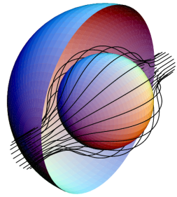
Figure 2: Rays traversing a spherical cloak. The transformation media that comprises the cloak lies between the two spheres.

For the spherical cloak (Fig.2), the Hamiltonian which yields the simplest equations is

$$H=\frac{1}{2}\frac{b-a}{b}\left(\mathbf{knk}-\det\left(\mathbf{n}\right)\right)$$ (46)

Plugging in the material properties from (22) and (23) we obtain

$$H=\frac{1}{2}\mathbf{k}\cdot\mathbf{k}-\frac{1}{2}\frac{2ar-a^{2}}{r^{4}}\left(\mathbf{x}\cdot\mathbf{k}\right)^{2}-\frac{1}{2}\left[\frac{b\left(r-a\right)}{r\left(b-a\right)}\right]^{2}$$

Taking the derivatives, (which is straight forward particularly in index form), yields

$$\frac{\partial H}{\partial\mathbf{k}} =\mathbf{k}-\frac{2ar-a^{2}}{r^{4}}\left(\mathbf{x}\cdot\mathbf{k}\right)\mathbf{x}$$ (47a)

$$\frac{\partial H}{\partial\mathbf{x}} =\left[\begin{array}[c]{c}-\frac{2ar-a^{2}}{r^{4}}\left(\mathbf{x}\cdot\mathbf{k}\right)\mathbf{k}+\frac{3ar-2a^{2}}{r^{6}}\left(\mathbf{x}\cdot\mathbf{k}\right)^{2}\mathbf{x}\\ -\left(\frac{b}{b-a}\right)^{2}\left(\frac{ar-a^{2}}{r^{4}}\right)\mathbf{x}\end{array}\right]$$ (47d)

V.2 Cylindrical Cloak

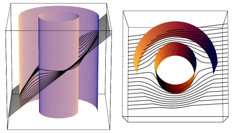
Figure 3: Rays traversing a cylindrical cloak at an oblique angle. The transformation media that comprises the cloak lies in an annular region between the cylinders.

For the cylindrical cloak (Fig.3), the Hamiltonian which yields the simplest equations is

$$H=\frac{1}{2}\frac{\rho-a}{\rho}\left(\mathbf{knk}-\det\left(\mathbf{n}\right)\right)$$ (48)

Plugging in the material properties form (30) and (31) we obtain

$$H=\frac{1}{2}\mathbf{kTk}-\frac{1}{2}\frac{2a\rho-a^{2}}{\rho^{4}}\left(\boldsymbol{\rho}\cdot\mathbf{k}\right)^{2}+\frac{1}{2}\left[\frac{b\left(\rho-a\right)}{\rho\left(b-a\right)}\right]^{2}\left(\mathbf{kZk}-1\right)$$ (49)

For taking the derivatives we note that the derivative of the transverse position vector with respect to the position vector is the transverse projection operator.

$$\frac{\partial\boldsymbol{\rho}}{\partial\mathbf{x}}=\mathbf{T}$$ (50)

The derivatives are thus

$$\frac{\partial H}{\partial\mathbf{k}} =\mathbf{Tk}-\frac{2a\rho-a^{2}}{\rho^{4}}\left(\boldsymbol{\rho}\cdot\mathbf{k}\right)\boldsymbol{\rho}+\left[\frac{b\left(\rho-a\right)}{\rho\left(b-a\right)}\right]^{2}\mathbf{Zk}$$ (51a)

$$\frac{\partial H}{\partial\mathbf{x}} =\left[\begin{array}[c]{c}\frac{3a\rho-2a^{2}}{\rho^{6}}\left(\boldsymbol{\rho}\cdot\mathbf{k}\right)^{2}\boldsymbol{\rho}-\frac{2a\rho-a^{2}}{\rho^{4}}\left(\mathbf{\rho\cdot k}\right)\mathbf{Tk}\\ +\left(\frac{b}{b-a}\right)^{2}\frac{a\rho-a^{2}}{\rho^{4}}\left(\mathbf{kZk}-1\right)\boldsymbol{\rho}\end{array}\right]$$ (51d)

VI Conclusion

We have shown how to calculate the material properties associated with a coordinate transformation and use these properties to perform ray tracing. Examples, of spherical and cylindrical cloaks are worked out in some detail. Some of the value in this effort is to provide independent confirmation that the material properties calculated from the transformation do indeed cause electromagnetic waves to behave in the desired and predicted manner. Eventually, this technique will become more accepted and independent confirmation will not be needed. One can see what the waves will do much more easily by applying the transformation to the rays or fields in the original space where the behavior is simpler if not trivial. However, one may still want to perform ray tracing on these media to see the effects of perturbations from the ideal material specification.

D. Schurig wishes to acknowledge the IC Postdoctoral Research Fellowship program.

References

- Pendry et al. (2006) J. Pendry, D. Schurig, and D. Smith, Science 312 (2006).
- Leonhardt (2006) U. Leonhardt, Science 312 (2006).
- Smith et al. (2004) D. R. Smith, J. B. Pendry, and M. C. K. Wiltshire, Science 305 (2004).
- Cubukcu et al. (2003a) E. Cubukcu, K. Aydin, E. Ozbay, S. Foteinopoulou, and C. M. Soukoulis, Nature 423 (2003a).
- Cubukcu et al. (2003b) E. Cubukcu, K. Aydin, E. Ozbay, S. Foteinopoulou, and C. M. Soukoulis, Phys. Rev. Lett. 91 (2003b).
- Yen et al. (2004) T. J. Yen, W. J. Padilla, N. Fang, D. C. Vier, D. R. Smith, J. B. Pendry, D. N. Basov, and X. Zhang, Science 303, 1494 (2004).
- Linden et al. (2004) S. Linden, C. Enkrich, M. Wegener, J. Zhou, T. Koschny, and C. M. Soukoulis, Science 306, 1351 (2004).
- Schurig et al. (2006) D. Schurig, J. Mock, and D. Smith, Applied Physics Letters 88, 041109 (2006), URL http://dx.doi.org/10.1063/1.2166681.
- Alu and Engheta (2005) A. Alu and N. Engheta, Physical Review E 72 (2005).
- Milton and Nicorovici (2006) G. W. Milton and N.-A. P. Nicorovici, Proc. Roy. Soc. London A 462 (2006).
- E.J.Post (1962) E.J.Post, Formal structure of electromagnetics (Wiley, New York, 1962).
- Jackson (1975) J. D. Jackson, Classical Electrodynamics (Wiley, New York, 1975).
- Kong (1990) J. A. Kong, Electromagnetic Wave Theory (Wiley-Interscience, New York, 1990), 2nd ed.
- Shyroki (2006) D. M. Shyroki (2006), unpublished.
- Ward and Pendry (1996) A. Ward and J. Pendry, Journal of Modern Optics 43, 773 (1996), URL http://dx.doi.org/10.1080/095003496155878.
- Leonhardt and Philbin (2006) U. Leonhardt and T. G. Philbin (2006), URL http://xxx.arxiv.org/abs/cond-mat/0607418.
- Yu.A.Kravtsov and Yu.I.Orlov (1990) Yu.A.Kravtsov and Yu.I.Orlov, Geometrical optics of inhomogeneous media (Springer-Verlag, Berlin, 1990).