30 June 2000

The Effect of Electric Fields In A Classic Introductory Physics Treatment of Eddy Current Forces

P.  J.  Salzman

Department of Physics
University of California
Davis, California 95616 USA
psalzman@dirac.org
John  Robert Burke

Department of Physics and Astronomy
San Francisco State University
San Francisco, California 94132 USA
burke@stars.sfsu.edu
Susan M. Lea

Department of Physics and Astronomy
San Francisco State University
San Francisco, California 94132 USA
lea@stars.sfsu.edu

Abstract

A simple model of eddy currents in which current is computed solely from magnetic forces acting on electrons proves accessible to introductory students and gives a good qualitative account of eddy current forces. However, this model cannot be complete; it ignores the electric fields that drive current outside regions of significant magnetic field. In this paper we show how to extend the model to obtain a boundary value problem for current density. Solution of this problem in polar coordinates shows that the electric field significantly affects the quantitative results and presents an exercise suitable for upper division students. We apply elliptic cylindrical coordinates to generalize the result and offer an exercise useful for teaching graduate students how to use non-standard coordinate systems.

1. Introduction

Every student of Electricity and Magnetism learns that Lenz’s Law predicts a force that opposes the motion of a conductor passing through a non-uniform magnetic field. Motion of the conductor’s free charge through the field results in magnetic forces that drive current in the conductor. This current, in turn, interacts with the $\vec{\mathbf{B}}$ field and results in a net magnetic force acting on the conductor. The current is called an eddy current.

A classic classroom demonstration of eddy currents is a swinging metallic pendulum that passes through the field of a strong magnet. Eddy currents within the conductor damp the oscillation rapidly. When the conductor is replaced by another with holes, the eddy currents are impeded from circulating and the damping effect becomes very small. The currents cease in this case because a Hall electric field develops that balances the magnetic force acting on the free charge.

We can estimate the eddy-current force acting on the conductor by using a few simplifying assumptions^,,. First, model the conductor as a very large plane sheet passing between circular magnet poles of radius $a$. Then, idealize the magnetic field as uniform in the cylindrical volume between the magnet poles and dropping abruptly to zero outside that volume. Figure 1 illustrates the model in a view perpendicular to the conducting sheet.

Figure 1: Magnetic field penetrating a circular portion of a moving conductor.

In this view, the magnetic field falls on a circular region of the conductor, is uniform within the circle, and is zero outside the circle. The conductor moves in the ${\bf\hat{x}}$ direction with speed $v_{0}$ and the magnetic field is given by $\vec{\mathbf{B}}=-B_{0}{\bf\hat{z}}$ within the circle of radius $a$. By Ohm’s Law, the current density is proportional to the force that drives it:

$$\vec{\mathbf{J}}=\sigma\vec{\mathbf{v}}\times\vec{\mathbf{B}}=\sigma vB\,{\bf\hat{z}},$$ (1a)

where $\sigma$ is the conductivity of the metal conductor. Then the force acting on a volume element $d\tau$ of the conductor within the field is:

$$d\vec{\mathbf{F}}=\vec{\mathbf{J}}\times\vec{\mathbf{B}}\,d\tau.$$

The net force acting on the conductor is

$$\vec{\mathbf{F}}=-\sigma v_{0}B_{0}^{2}V{\bf\hat{x}},$$ (1b)

where $V$ is the volume of the conductor exposed to the field.

This calculation correctly illustrates Lenz’s Law and the dependence of the force on velocity and magnetic field strength. So, it gives a useful back-of-the-envelope estimate for the eddy current force. However, it is a somewhat naive estimate. Once the current leaves the vicinity of the $\vec{\mathbf{B}}$ field, the model does not explain what causes the flow of free charge. It lacks an account of the Hall electric field (arising from charge distribution on the surface of discontinuity of $\vec{\mathbf{B}}$) which drives the current outside the $\vec{\mathbf{B}}$-field region, thus completing the current loops. This $\vec{\mathbf{E}}$ field also opposes the current flow within the $\vec{\mathbf{B}}$-field region, indicating that equation (1b) overestimates the force. In this paper we develop a method to account for this effect, and so to improve the estimate.

2. The Exact Circle Problem

Calculating the charge densities that give rise to electric fields driving current in conductors is notoriously difficult, but is usually not necessary. Here we can develop the calculation of current density as a two dimensional boundary-value problem using polar coordinates in the rest frame of the magnets. We retain the simple model of the magnetic field from the introduction and, for now, model the plate as infinite in the dimensions perpendicular to the field. We also assume that the plate’s speed is sufficiently small that we can model the current distribution as a quasi-steady state in the magnet frame. The resulting problem is a challenging but accessible problem for upper division E&M students. In classic form, we observe that the current density is derivable from a potential that satisfies Laplace’s equation except at the magnetic field boundary, develop the appropriate boundary conditions and solve via expansion in eigenfunctions.

Then, the current density throughout is determined by Ohm’s Law:

$$\vec{\mathbf{J}}=\sigma\left(\vec{\mathbf{E}}+\vec{\mathbf{v}}\times\vec{\mathbf{B}}\right).$$

Taking the curl of both sides and using a vector identity for ${\vec{\mathbf{\boldsymbol{\nabla}}}}\times(\vec{\mathbf{v}}\times\vec{\mathbf{B}})$ yields:

$$\vec{\mathbf{\boldsymbol{\nabla}}}\times\vec{\mathbf{J}}=-\sigma(\vec{\mathbf{v}}\cdot\vec{\mathbf{\boldsymbol{\nabla}}})\vec{\mathbf{B}}.$$ (2.1)

Here we used the fact that the conductor’s velocity and $\vec{\mathbf{B}}$ are constant vectors in the magnet frame. Inserting the assumed form for $\vec{\mathbf{B}}$ and using polar coordinates for $\vec{\mathbf{\boldsymbol{\nabla}}}$, equation (2.1) can be rewritten as:

$$\vec{\mathbf{\boldsymbol{\nabla}}}\times\vec{\mathbf{J}}=-\sigma v_{0}B_{0}\cos(\phi)\delta(\rho-a){\bf\hat{z}},$$ (2.2)

where $\rho$ is the radial coordinate with origin at the center of the magnetic field region. Next, since no charge buildup is expected with time, the equation of continuity demands that $\vec{\mathbf{J}}$ be divergence free:

$${\vec{\mathbf{\boldsymbol{\nabla}}}}\cdot\vec{\mathbf{J}}=0.$$ (2.3)

Since the current density is curl free except at $\rho=a$, it is the gradient of some scalar potential on each side of $a$: $\vec{\mathbf{J}}_{\scriptscriptstyle>}=-{\vec{\mathbf{\boldsymbol{\nabla}}}}\Phi_{\scriptscriptstyle>}$ and $\vec{\mathbf{J}}_{\scriptscriptstyle<}=-{\vec{\mathbf{\boldsymbol{\nabla}}}}\Phi_{\scriptscriptstyle<}$, where the subscripts $>$ and $<$ refer respectively to regions outside and inside the boundary. Thus ${\vec{\mathbf{\boldsymbol{\nabla}}}}^{2}\Phi=0$ everywhere except at the magnetic field boundary, and we may proceed with standard methods for solving Laplace’s equation.

The boundary conditions on the components of $\vec{\mathbf{J}}$ perpendicular and parallel to the boundary follow from the divergence and curl of current density. This is a standard calculation, with the results

$$J_{\scriptscriptstyle>,\perp}(a^{\scriptscriptstyle+})-J_{\scriptscriptstyle<,\perp}(a^{\scriptscriptstyle-})=0;$$

$$J_{\scriptscriptstyle<,\parallel}(a^{\scriptscriptstyle+})-J_{\scriptscriptstyle<,\parallel}(a^{\scriptscriptstyle-})=-\sigma v_{0}B_{0}\cos(\phi).$$

In terms of potential, the boundary conditions are:

$$\partial_{\rho}\Phi_{\scriptscriptstyle>}(\rho=a^{\scriptscriptstyle+})-\partial_{\rho}\Phi_{\scriptscriptstyle<}(\rho=a^{\scriptscriptstyle-})=0;$$ (5a)

$$\partial_{\phi}\Phi_{\scriptscriptstyle>}(\rho=a^{\scriptscriptstyle+})-\partial_{\phi}\Phi_{\scriptscriptstyle<}(\rho=a^{\scriptscriptstyle-})=\sigma av_{0}B_{0}\cos(\phi).$$ (5b)

The problem is now completely specified, and we proceed by expanding the potential in eigenfunctions of the Laplace operator in polar coordinates.

$$\Phi(\vec{\mathbf{x}})=\begin{cases}\Phi_{\scriptscriptstyle<}=\sum_{n=0}^{\infty}\rho^{n}\left[A_{n}\sin(n\phi)+B_{n}\cos(n\phi)\right]&\rho<a\\ \Phi_{\scriptscriptstyle>}=\sum_{n=0}^{\infty}\rho^{-n}\left[A_{n}\sin(n\phi)+B_{n}\cos(n\phi)\right]&\rho>a.\end{cases}$$ (2.5)

From the boundary condition for $J_{\scriptscriptstyle\parallel}$ (eqn 5b) and the orthogonality of the trigonometric functions, we see that the $n=1$ terms are the only non-zero terms in the sums. Furthermore, only the $A$ coefficients are non-zero. The boundary conditions on the potential now give two equations for the coefficients. We find:

$$\Phi(\vec{\mathbf{x}})=\begin{cases}\Phi_{\scriptscriptstyle<}=-\frac{1}{2}\sigma v_{0}B_{0}\rho\sin(\phi)&\rho<a\\ \Phi_{\scriptscriptstyle>}=+\frac{1}{2}\sigma v_{0}B_{0}\frac{a^{2}}{\rho}\sin(\phi)&\rho>a.\end{cases}$$

We can take gradients to obtain the current density:

$$\vec{\mathbf{J}}(\vec{\mathbf{x}})=\begin{cases}\vec{\mathbf{J}}_{\scriptscriptstyle<}=-{\vec{\mathbf{\boldsymbol{\nabla}}}}\Phi_{\scriptscriptstyle<}=\frac{1}{2}\sigma v_{0}B_{0}\,\boldsymbol{{\bf\hat{y}}}&\rho<a\\ \vec{\mathbf{J}}_{\scriptscriptstyle>}=-{\vec{\mathbf{\boldsymbol{\nabla}}}}\Phi_{\scriptscriptstyle>}=\frac{1}{2}\sigma v_{0}B_{0}\left(\frac{a}{\rho}\right)^{2}\left[\sin(\phi)\boldsymbol{{\bf\hat{\boldsymbol{\rho}}}}-\cos(\phi)\boldsymbol{{\bf\hat{\boldsymbol{\phi}}}}\right]&\rho>a.\end{cases}$$ (2.6)

We still find a uniform current density within the magnetic field region. The current outside the field region follows a classic dipole pattern. The corresponding electric field that drives current in the region $\rho>a$ and opposes it in the region $\rho<a$ is found from

$$\vec{\mathbf{E}} =\frac{\vec{\mathbf{J}}}{\sigma}-\vec{\mathbf{v}}\times\vec{\mathbf{B}}$$ (2.7)

$$=\begin{cases}-\frac{1}{2}v_{0}B_{0}\,\boldsymbol{{\bf\hat{y}}}&\rho<a\\[5.0pt] \frac{1}{2}v_{0}B_{0}\left(\frac{a^{2}}{\rho}\right)\left[\sin(\phi)\,\boldsymbol{{\bf\hat{\boldsymbol{\rho}}}}-\cos(\phi)\,\boldsymbol{{\bf\hat{\boldsymbol{\phi}}}}\right]&\rho>a\end{cases}$$ (2.8)

The charge density $\sigma_{c}$ that gives rise to this field is localized at $\rho=a$ and is found from the standard boundary condition:

$$\sigma_{c} =\varepsilon_{0}\,\boldsymbol{{\bf\hat{\boldsymbol{\rho}}}}\cdot\left[\vec{\mathbf{E}}_{>}-\vec{\mathbf{E}}_{<}\right]$$ (2.9)

$$=\varepsilon_{0}v_{0}B_{0}\sin(\phi)$$ (2.10)

For a field $B_{0}=1$T and a plate speed of $v_{0}=1\,$m/s, the charge density is of order $\sigma_{c}\sim 10^{-11}$ C/m².

Comparison equation (2.6) with equation (1a) shows that the current, and hence the net force acting on the conductor is half that predicted by the naive model. Such a simple result, in contrast with the complex correction one might have expected, rasies the issue whether a correction factor of $1/2$ is generally correct or specific to the circuclar field geometry. We investigate that question in the following sections.

3. Elliptical Magnetic Field Region

The result for a circular magnetic field geometry demonstrates that electric field has a significant effect on eddy current flow. We were intrigued whether the factor of 1/2 reduction is a general result or special to the case of circular geometry. To investigate this question, we solved the problem of an elliptically shaped magnetic field region with eccentricity $\epsilon$, as shown in Figure 2. The method follows the same outline as the circle problem except that we expand the potential in elliptic cylindrical coordinates, defined^, in terms of Cartesian by:

$$x=h\cosh(\eta)\cos(\psi)\qquad y=h\sinh(\eta)\sin(\psi)\qquad z=z.$$ (3.1)

The unit vectors are given by

$${\bf\hat{x}}=\frac{\boldsymbol{{\bf\hat{\boldsymbol{\eta}}}}\sinh(\eta)\cos(\psi)-\boldsymbol{{\bf\hat{\boldsymbol{\psi}}}}\cosh(\eta)\sin(\psi)}{\sqrt{\cosh^{2}(\eta)-\cos^{2}(\psi)}}\qquad{\bf\hat{y}}=\frac{\boldsymbol{{\bf\hat{\boldsymbol{\eta}}}}\cosh(\eta)\sin(\psi)+\boldsymbol{{\bf\hat{\boldsymbol{\psi}}}}\sinh(\eta)\cos(\psi)}{\sqrt{\cosh^{2}(\eta)-\cos^{2}(\psi)}}.$$ (3.2)

The constant $h$ is the product of the semi-major axis $a$ and eccentricity $\epsilon$ of the elliptical magnetic field region. The boundary of the magnetic field is defined by the level curve

$$\eta=\eta_{0}=\cosh^{-1}\left(\frac{1}{\epsilon}\right).$$ (3.3)

Figure 2: The magnetic field penetrates an elliptical portion of a moving conductor. The level curves of coordinate $\eta$ are ellipses with foci $p$ and $q$, a distance $2h$ apart. The level curves of $\psi$ are semi-hyperbolae; the value of $\psi$ is the polar angle of the asymptote. The boundary of the magnetic field is given by $\eta=\eta_{0}=\cosh^{-1}(\frac{1}{\epsilon})$. The semi-major axis of the boundary is $a$.

In these coordinates, the vector expressions for the divergence and curl of $\vec{\mathbf{J}}$ are unchanged:

$${\vec{\mathbf{\boldsymbol{\nabla}}}}\cdot\vec{\mathbf{J}}=0\qquad{\vec{\mathbf{\boldsymbol{\nabla}}}}\times\vec{\mathbf{J}}=-\sigma(\vec{\mathbf{v}}\cdot{\vec{\mathbf{\boldsymbol{\nabla}}}})\,\vec{\mathbf{B}}(\eta)$$

where $\vec{\mathbf{B}}=-B_{0}{\bf\hat{z}}$ within the field region and zero outside. Using equation (3.2) we may express $(\vec{\mathbf{v}}\cdot{\vec{\mathbf{\boldsymbol{\nabla}}}})\vec{\mathbf{B}}$ in this coordinate system. We find:

$${\vec{\mathbf{\boldsymbol{\nabla}}}}\times\vec{\mathbf{J}} =-\frac{\sigma v_{0}\sinh(\eta)\cos(\psi)}{h[\cosh^{2}(\eta)-\cos^{2}(\psi)]}\frac{\partial\vec{\mathbf{B}}(\eta)}{\partial\eta},$$

$$=-\frac{\sigma v_{0}B_{0}\sinh(\eta)\cos(\psi)}{h[\cosh^{2}(\eta)-\cos^{2}(\psi)]}\delta(\eta-\eta_{0})\,{\bf\hat{z}}.$$

As before, conditions on the curl and divergence of $\vec{\mathbf{J}}$ lead to boundary conditions:

$$J_{\scriptscriptstyle>,\perp}(\eta_{0})-J_{\scriptscriptstyle<,\perp}(\eta_{0}) =0,$$

$$J_{\scriptscriptstyle>,\parallel}(\eta_{0})-J_{\scriptscriptstyle<,\parallel}(\eta_{0}) =-\frac{\sigma v_{0}B_{0}\sinh(\eta_{0})\cos(\psi)}{\sqrt{\cosh^{2}(\eta_{0})-\cos^{2}(\psi)}}.$$

Once again we can make the argument that $\vec{\mathbf{J}}$ is the gradient of some scalar potential $\Phi$ in the regions separated by $\eta=\eta_{0}$. That is, $\vec{\mathbf{J}}_{\scriptscriptstyle<}=-{\vec{\mathbf{\boldsymbol{\nabla}}}}\Phi_{\scriptscriptstyle<}$ for $\eta<\eta_{0}$ and $\vec{\mathbf{J}}_{\scriptscriptstyle>}=-{\vec{\mathbf{\boldsymbol{\nabla}}}}\Phi_{\scriptscriptstyle>}$ for $\eta>\eta_{0}$. Components of current which lie perpendicular and parallel to the curve bounding the $\vec{\mathbf{B}}$ region are then given by:

$$J_{\scriptscriptstyle\perp} =-{\vec{\mathbf{\boldsymbol{\nabla}}}}\Phi\cdot\boldsymbol{{\bf\hat{\boldsymbol{\eta}}}}=-\frac{1}{h\sqrt{\cosh^{2}(\eta)-\cos^{2}(\psi)}}\frac{\partial\Phi}{\partial\eta},$$

$$J_{\scriptscriptstyle\parallel} =-{\vec{\mathbf{\boldsymbol{\nabla}}}}\Phi\cdot\boldsymbol{{\bf\hat{\boldsymbol{\psi}}}}=-\frac{1}{h\sqrt{\cosh^{2}(\eta)-\cos^{2}(\psi)}}\frac{\partial\Phi}{\partial\psi}.$$

The boundary conditions on $\vec{\mathbf{J}}$ then give us the following boundary conditions on the potential:

$$\partial_{\psi}\Phi_{\scriptscriptstyle>}(\eta=\eta^{\scriptscriptstyle+}_{0})-\partial_{\psi}\Phi_{\scriptscriptstyle<}(\eta=\eta^{\scriptscriptstyle-}_{0}) =\sigma hv_{0}B_{0}\sinh(\eta_{0})\cos(\psi),$$

$$\partial_{\eta}\Phi_{\scriptscriptstyle>}(\eta=\eta^{\scriptscriptstyle+}_{0})-\partial_{\eta}\Phi_{\scriptscriptstyle<}(\eta=\eta^{\scriptscriptstyle-}_{0}) =0.$$

The expansion of the potential in terms of eigenfunctions of the Laplace operator in this coordinate system is:

$$\Phi(\vec{\mathbf{x}})=\begin{cases}\Phi_{\scriptscriptstyle<}=\sum_{n=0}^{\infty}\left[E_{n}\sinh(n\eta)+F_{n}\cosh(n\eta)\right]\left[A_{n}\sin(n\psi)+B_{n}\cos(n\psi)\right]&\eta<\eta_{0}\\[5.0pt] \Phi_{\scriptscriptstyle>}=\sum_{n=0}^{\infty}\left[G_{n}e^{n\eta}+H_{n}e^{-n\eta}\right]\left[C_{n}\sin(n\psi)+D_{n}\cos(n\psi)\right]&\eta>\eta_{0}.\end{cases}$$ (3.4)

Once again, orthogonality of the trigonometric functions ensures that only $n=1$ terms will be non-zero. In the limit $\eta\rightarrow\infty$, we require $\Phi_{\scriptscriptstyle>}$ to remain finite, so we have $G_{1}=0$. The limit $\eta\rightarrow 0$ describes the portion of the x-axis between the two foci. Here the curl and divergence of $\vec{\mathbf{J}}$ are both zero, so that $\vec{\mathbf{J}}$ is continuous across the x-axis. Since $\eta$ increases away from the x-axis on both sides, $\boldsymbol{{\bf\hat{\boldsymbol{\eta}}}}$ changes direction discontinuously across the x-axis. Thus, continuity of $J_{\scriptscriptstyle\perp}$ implies that $J_{\eta}\propto\partial_{\eta}\Phi_{\scriptscriptstyle<}$ changes sign across the x-axis. This fact requires that the $\cos(\psi)$ term in $\Phi_{\scriptscriptstyle<}$ be zero since only $\sin(\psi)$ is discontinuous at $y=0$. Now, $\boldsymbol{{\bf\hat{\boldsymbol{\psi}}}}$ is also discontinuous across the x-axis between the foci, so continuity of $J_{\scriptscriptstyle\parallel}$ requires that $\partial_{\psi}\Phi_{\scriptscriptstyle<}\propto\cos(\psi)$ either be discontinuous (which it isn’t) or be zero. Thus $\partial_{\psi}\Phi_{\scriptscriptstyle<}=0$ as $\eta\rightarrow 0$, which requires that $F_{1}=0$. Then, the boundary conditions at $\eta_{0}$ require

$$\Phi(\vec{\mathbf{x}})=\begin{cases}\Phi_{\scriptscriptstyle<}=-\frac{\sigma hv_{0}B_{0}\sinh(\eta_{0})}{\cosh(\eta_{0})+\sinh(\eta_{0})}\sinh(\eta)\sin(\psi)&\eta<\eta_{0}\\ \Phi_{\scriptscriptstyle>}=\sigma hv_{0}B_{0}\sinh(\eta_{0})\cosh(\eta_{0})e^{-\eta}\sin(\psi)&\eta>\eta_{0}.\end{cases}$$

We can take gradients to calculate the exact current density:

$$\vec{\mathbf{J}}(\vec{\mathbf{x}})=\begin{cases}\vec{\mathbf{J}}_{\scriptscriptstyle<}=\frac{\sigma v_{0}B_{0}\sinh(\eta_{0})}{\cosh(\eta_{0})+\sinh(\eta_{0})}\,\boldsymbol{{\bf\hat{y}}}&\eta<\eta_{0}\\ \vec{\mathbf{J}}_{\scriptscriptstyle>}=\sigma v_{0}B_{0}\sinh(\eta_{0})\cosh(\eta_{0})e^{-\eta}\left(\frac{\boldsymbol{{\bf\hat{\boldsymbol{\eta}}}}\sin(\psi)-\boldsymbol{{\bf\hat{\boldsymbol{\psi}}}}\cos(\psi)}{\sqrt{\cosh^{2}(\eta)-\cos^{2}(\psi)}}\right)&\eta>\eta_{0}.\end{cases}$$ (3.5)

Substituting for $\eta_{0}$ in terms of the $\vec{\mathbf{B}}$-field region’s eccentricity (eqn 3.3) we find:

$$\vec{\mathbf{J}}(\vec{\mathbf{x}})=\begin{cases}\vec{\mathbf{J}}_{\scriptscriptstyle<}=\sigma v_{0}B_{0}\frac{\sqrt{1-\epsilon^{2}}}{1+\sqrt{1-\epsilon^{2}}}\,\boldsymbol{{\bf\hat{y}}}&\eta<\cosh^{-1}(1/\epsilon)\\ \vec{\mathbf{J}}_{\scriptscriptstyle>}=\sigma v_{0}B_{0}\frac{\sqrt{1-\epsilon^{2}}}{\epsilon^{2}}e^{-\eta}\left(\frac{\boldsymbol{{\bf\hat{\boldsymbol{\eta}}}}\sin(\psi)-\boldsymbol{{\bf\hat{\boldsymbol{\psi}}}}\cos(\psi)}{\sqrt{\cosh^{2}(\eta)-\cos^{2}(\psi)}}\right)&\eta>\cosh^{-1}(1/\epsilon).\end{cases}$$ (3.6)

Again we find uniform current density in the magnetic field region. The factor of 1/2 reduction in current density found for the circular field turns out not to be general. It is replaced by the factor

$$\frac{\sqrt{1-\epsilon^{2}}}{1+\sqrt{1-\epsilon^{2}}},$$

which, of course, has the limit $1/2$ as $\epsilon\rightarrow 0$. The graph of this function is shown as Figure 3. Since the force acting on the sheet is $\vec{\mathbf{F}}_{net}=-B_{0}|\vec{\mathbf{J}}_{\scriptscriptstyle<}|V\,{\bf\hat{x}}$ where $V$ is the volume exposed to the magnetic field, the force also has the expected limit. It is much more intricate and much less crucial to establish that the expression for $\vec{\mathbf{J}}_{\scriptscriptstyle>}$ reduces to the circular results in the limit $\epsilon\rightarrow 0$. The calculation is not given here, but a copy of it is available from the authors upon request.

4. The Effect Of Finite Conductor Size

Once these two calculations are set up for infinite plates, it is easy to estimate the correction for finite plate size. One changes the boundary condition from $|\vec{\mathbf{J}}_{\scriptscriptstyle>}|\rightarrow 0$ at infinity to vanishing of the radial component of $\vec{\mathbf{J}}_{\scriptscriptstyle>}$ at a finite radial coordinate.

For the circular case we take the plate to have a finite radius $R$. A solution is only feasible for the time when the plate is centered on the magnetic field region, so the result offers only an order of magnitude estimate of the effects.

In eqn (2.5) (the expansion of the potential) an extra term in $\Phi_{\scriptscriptstyle>}$ that increases with $\rho$ is necessary to match the new boundary condition. A straightforward calculation reveals:

$$\vec{\mathbf{J}}(\vec{\mathbf{x}})=\begin{cases}\frac{1}{2}\sigma v_{0}B_{0}\left(1-\frac{a^{2}}{R^{2}}\right)\boldsymbol{{\bf\hat{y}}}&\rho<a\\[5.0pt] \frac{1}{2}\sigma v_{0}B_{0}\left(\frac{a}{\rho R}\right)^{2}\left[(R^{2}-\rho^{2})\sin(\phi)\boldsymbol{{\bf\hat{\boldsymbol{\rho}}}}-(R^{2}+\rho^{2})\cos(\phi)\boldsymbol{{\bf\hat{\boldsymbol{\phi}}}}\right]&R>\rho>a.\end{cases}$$ (4.1)

One may quickly verify that these expressions have the correct limits (eqn 2.6) in the infinite conductor case ($R\rightarrow\infty$). The effect on the dipole current term is substantial near the boundary. Current in the magnetic field region is further reduced by the edge effects, but by an insubstantial amount, unless the distance from the center to the nearest edge is comparable to the radius of the field region.

A similar calculation is possible for elliptic cylindrical coordinates with a border at $\eta=H$ (semi-major axis of the boundary is $A=a\epsilon\cosh(H)$. As in circular geometry, we augment the old conditions with the new condition that the elliptic-radial component of $\vec{\mathbf{J}}_{\scriptscriptstyle>}$ vanishes at the boundary: $\partial_{\eta}\Phi(H,\psi)=0$. We find:

$$\vec{\mathbf{J}}_{\scriptscriptstyle<}(\vec{\mathbf{x}})=\sigma v_{0}B_{0}\frac{\sqrt{1-\epsilon^{2}}}{\epsilon^{2}}\left(\sqrt{1-\left(\frac{a\epsilon}{A}\right)^{2}}-\sqrt{1-\epsilon^{2}}\right)\qquad\eta<\cosh^{-1}(\frac{1}{\epsilon}).$$

Observing that $\sqrt{1-\epsilon^{2}}/(1+\sqrt{1-\epsilon^{2}})=\sqrt{1-\epsilon^{2}}(1-\sqrt{1-\epsilon^{2}})/\epsilon^{2}$, we see that the effect on $\vec{\mathbf{J}}_{\scriptscriptstyle<}$ is to replace $1$ with $\sqrt{1-\left(\frac{a\epsilon}{A}\right)^{2}}$ in the last factor of the expression. Again the correction is of order of the square of the ratio of magnet size to the plate dimension.

5. Conclusion

We have demonstrated that the electric field has a significant effect on the eddy-current force computed from a simple model. The model gives the magnitude of the force as

$$F=\sigma v_{0}B_{0}^{2}Vf,$$ (5.1)

where $V$ is the volume of conductor exposed to the magnetic field $B_{0}$, $\sigma$ is the conductivity of the metal and $v_{0}$ is its speed relative to the source of the magnetic field. The factor $f$ is the correction due to the electric field; $1/2$ for an infinite metal plate and circular magnet poles and $\sqrt{1-\epsilon^{2}}/(1+\sqrt{1-\epsilon^{2}})$ for an infinite metal plate with elliptical magnetic poles.

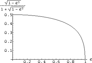
Figure 3: The reduction factor in the current density for an arbitrary ellipse as a function of the ellipse’s eccentricity.

The first result follows from a boundary value problem accessible to an upper division student, while the second result requires boundary value techniques that would be good training for a graduate student. Corrections for finite plate size alter the result by terms of order (magnet size / plate size)².

A possible objection to this method is the need for assuming an abrupt edge to the magnetic field region. Burke and Lea have developed a method for treating a more realistic model of the field. In the limit of zero separation of the magnet poles they find $f=1/2$. For a pole separation of one-tenth of the pole radius, they find $f=0.39266$.

In all cases, $0\leq f\leq 0.5$, though $0.5$ seems to be a robust approximation.

6. Acknowledgements

This work was supported in part by the Department of Energy under grant DE-FG03-91ER40674. It was also supported in part by The Portland Group, Inc. (PGI) for the generous use of the PGI Workstation.