Lead-lag cross-sectional structure and detection of correlated-anticorrelated regime shifts: application to the volatilities of inflation and economic growth rates

Abstract

We have recently introduced the “thermal optimal path” (TOP) method to investigate the real-time lead-lag structure between two time series. The TOP method consists in searching for a robust noise-averaged optimal path of the distance matrix along which the two time series have the greatest similarity. Here, we generalize the TOP method by introducing a more general definition of distance which takes into account possible regime shifts between positive and negative correlations. This generalization to track possible changes of correlation signs is able to identify possible transitions from one convention (or consensus) to another. Numerical simulations on synthetic time series verify that the new TOP method performs as expected even in the presence of substantial noise. We then apply it to investigate changes of convention in the dependence structure between the historical volatilities of the USA inflation rate and economic growth rate. Several measures show that the new TOP method significantly outperforms standard cross-correlation methods.

,

1 Introduction

The study of the lead-lag structure between two time series $X(t)$ and $Y(t)$ has a long history, especially in economics, econometrics and finance, as it is often asked which economic variable might influence other economic phenomena. A simple measure is the lagged cross-correlation function $C_{X,Y}(\tau)=\langle X(t)Y(t+\tau)\rangle/\sqrt{{\rm Var}[X]{\rm Var}[Y]}$, where the brackets $\langle x\rangle$ denotes the statistical expectation of the random variable $x$ and ${\rm Var}[x]$ is the variance of $x$. The observation of a maximum of $C_{X,Y}(\tau)$ at some non-zero positive time lag $\tau$ implies that the knowledge of $X$ at time $t$ gives some information on the future realization of $Y$ at the later time $t+\tau$. However, such correlations do not imply necessarily causality in a strict sense as a correlation may be mediated by a common source influencing the two time series at different times. The concept of Granger causality bypasses this problem by taking a pragmatic approach based on predictability: if the knowledge of $X(t)$ and of its past values improves the prediction of $Y(t+\tau)$ for some $\tau>0$, then it is said that $X$ Granger causes $Y$ (see, e.g., [1, 2, 3]). Such a definition does not address the fundamental philosophical and epistemological question of the real causality links between $X$ and $Y$ but has been found useful in practice. Our approach is similar in that it does not address the question of the existence of a genuine causality but attempts to detect a dependence structure between two time series at non-zero (possibly varying) lags. We thus use the term “causality” in a loose sense embodying the notion of a dependence between two time series with a non-zero lag time.

Many alternative methods have been developed in the physical community. Quiroga et al. proposed a simple and fast method to measure synchronicity and time delay patterns between two time series based on event synchronization [4]. Furthermore, as a generalization of the concept of recurrence plot to analyze complex chaotic time series [5], Marwan et al. developed cross-recurrence plot based on a distance matrix to unravel nonlinear mapping of times between two systems [6, 7]. In Ref. [8], we have introduced a novel non-parametric method to test for the dynamical time evolution of the lag-lead structure between two arbitrary time series based on a thermal averaging of optimal paths embedded in the distance matrix previously introduced in cross-recurrence plots. This method ignores the thresholds used previously in constructing cross recurrence plot [6, 7] and focuses on the distance matrix. The idea consists in constructing a distance matrix based on the matching of all sample data pairs obtained from the two time series under study. The lag-lead structure is searched for as the optimal path in the distance matrix landscape that minimizes the total mismatch between the two time series, and that obeys a one-to-one causal matching condition. To make the solution robust with respect to the presence of noise that may lead to spurious structures in the distance matrix landscape, Sornette and Zhou generalized this search for a single absolute optimal path by introducing a fuzzy search consisting in sampling over all possible paths, each path being weighted according to a multinomial logit or equivalently Boltzmann factor proportional to the exponential of the global mismatch of this path [8]. The method is referred to in the sequel as the thermal optimal path (TOP). Zhou and Sornette investigated further the TOP method by considering difference topologies of feasible paths and found that the two-layer scheme gives the best performance [9].

Here, we generalize the TOP method by introducing a definition of distance which takes into account possible regime shifts between positive and negative correlations. This extension allows us to detect possible changes in the sign of the correlation between the two time series. This is in part motivated by the problem of identifying changes of conventions in economic and financial time series. Keynes [10] and Orléan [11, 12, 13, 14, 15, 16, 17] developed the concept of convention, according to which a pattern can emerge from the self-fulfilling belief of agents acting on the belief itself. Conventions are subject to shifts: in a recent study, Wyart and Bouchaud claimed that the correlation between bond markets and stock markets was positive in the past (because low long term interest rates should favor stocks), but has recently quite suddenly become negative as a new “Flight To Quality” convention has set in: selling risky stocks and buying safe bonds has recently been the dominant pattern [18]. Similarly, Liu and Liu analyzed the nexus between the historical volatility of the output and of the inflation rate, using Chinese data from 1992 to 2004 [19]. They found that there is a strong correlation between the two volatilities and, what is more interesting, that the rolling correlation coefficient changes sign. Such a change of sign of the correlation may be attributed either to a shift in convention and/or to changing macroeconomic variables, the two being possible entangled. Our method does not address the source of the change of the sign of the correlation but provides nevertheless a preliminary tool for detecting such changes of correlations in an time-adaptive lead-lag framework.

The paper is organized as follows. In Section 2, we present a brief description of our generalized TOP method. We recall that an advantage of the TOP method is that it does not require any a priori knowledge of the underlying dynamics. The new TOP method is illustrated with the help of synthetic numerical simulations in Section 3. Section 4 presents the application of the method to the investigation of a possible change of dependence between the historical volatility of the USA inflation rate and the economic growth rate. Section 5 concludes.

2 Thermal optimal path method

In Refs.[8, 9], we have presented the TOP method and several tests and applications. In this section, to be self-contained, we briefly recall its main characteristics in the context of the new proposed distance.

Consider two standardized time series $\{X(t_{1}):t_{1}=0,...,N\}$ and $\{Y(t_{2}):t_{2}=0,...N\}$. The elements of the distance matrix $E_{X,Y}$ between $X$ to $Y$ used in Refs. [8, 9] are defined as

$$\epsilon_{-}(t_{1},t_{2})=[X(t_{1})-Y(t_{2})]^{2}~{}.$$ (1)

The value $[X(t_{1})-Y(t_{2})]^{2}$ defines the distance between the realizations of the first time series at time $t_{1}$ and the second time series at time $t_{2}$.

The distance matrix (1) tracks the co-monotonic relationship between $X$ and $Y$. But, two time series can be more anti-monotonic than monotonic, i.e., they tend to take opposite signs. Consider two limiting cases: (i) $Y(t)=X(t)$ and (ii) $Y(t)=-X(t)$. Obviously, using the traditional distance (1) identifies case (i) as minimizing expression (1) for $t_{1}=t_{2}$ (actually the minimum is identically zero in this special case). In contrast, notwithstanding the fact that $Y(t)$ is perfectly (anti-)correlated with $X(t)$, the naive idea of minimizing the distance (1) between the two time series becomes meaningless. In order to diagnose the occurrence of anti-correlation, one needs to consider the “anti-monotonic” distance

$$\epsilon_{+}(t_{1},t_{2})=[X(t_{1})+Y(t_{2})]^{2}~{}.$$ (2)

The $+$ sign ensures a correct search of synchronization between two anti-correlated time series. More generally, $X$ and $Y$ may exhibit more complicated lead-lag correlation relationships, positive correlation over some time intervals and negative correlation at other times (as in the change of conventions mentioned in the introduction). In order to address all possible situations, we propose to use the mixed distance expressed as follows:

$$\epsilon_{\pm}(t_{1},t_{2})=\min[\epsilon_{-}(t_{1},t_{2}),\epsilon_{+}(t_{1},t_{2})]~{}.$$ (3)

Fig. 1 is a schematic representation of how lead-lag paths are defined. The first (resp. second) time series is indexed by the time $t_{1}$ (resp. $t_{2}$). The nodes of the plane carry the values of the distance (3) for each pair $(t_{1},t_{2})$. The path along the diagonal corresponds to taking $t_{1}=t_{2}$, i.e., compares the two time series at the same time. Paths below (resp. above) the diagonal correspond to the second time series lagging behind (resp. leading) the first time series. The figure shows three arrows which define the three causal steps (time flows from the past to the future both for $t_{1}$ and $t_{2}$) allowed in our construction of the lead-lag paths. A given path selects a contiguous set of nodes from the lower left to the upper right. The relevance or quality of a given path with respect to the detection of the lead-lag relationship between the two time series is quantified by the sum of the distances (3) along its length.

As shown in the figure, it is convenient to use the rotated coordinate system $(x,t)$ such that

$$\left\{\begin{array}[]{ccl}t_{1}&=&1+\left(t-x\right)/2{}\\ t_{2}&=&1+\left(t+x\right)/2{}\end{array}\right.,$$ (4)

where $t$ is in the main diagonal direction of the $(t_{1},t_{2})$ system and $x$ is perpendicular to $t$. The origin $(x=0,t=0)$ corresponds to $(t_{1}=1,t_{2}=1)$. Then, the standard reference path is the diagonal of equation $x=0$, and paths which have $x(t)\neq 0$ define varying lead-lag patterns. The idea of the TOP method is to identify the lead-lag relationship between two time series as the best path in a certain sense. One could first infer that the best path is the one which has the minimum sum of its distances (3) along its length (paths are constructed with equal lengths so as to be comparable). The problem with this idea is that the noises decorating the two time series introduce spurious patterns which may control the determination the path which minimizes the sum of distances, leading to incorrect inferred lead-lag relationships. In Refs.[8, 9], we have shown that a robust lead-lag path is obtained by defining an average over many paths, each weighted according to a Boltzmann-Gibbs factor, hence the name “thermal” optimal path method.

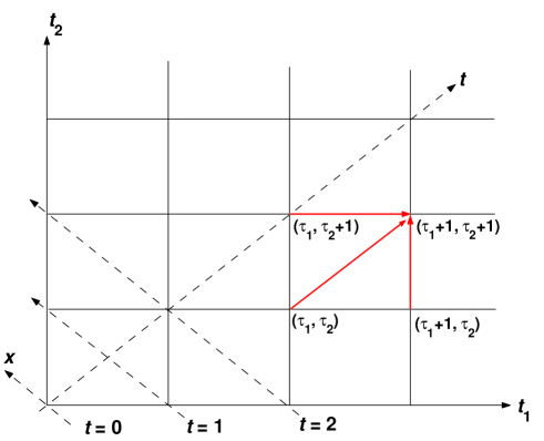
Figure 1: (Color online) Representation of the two-layer approach in the lattice $(t_{1},t_{2})$ and of the rotated frame $(t,x)$ as defined in the text. The three arrows depict the three moves that are allowed to reach any node in one step.

Concretely, we first calculate the partition functions $G(x,t)$ and their sum $G(t)=\sum_{x}G(x,t)$ so that $G(x,t)/G(t)$ can be interpreted as the probability for a path to be at distance $x$ from the diagonal for a distance $t$ along the diagonal. This probability $G(x,t)/G(t)$ is determined as a compromise between minimizing the mismatch (similar to an “energy”) and maximizing the combinatorial weight of the number of paths with similar mismatchs in a neighborhood (similar to an “entropy”). As illustrated in Figure 1, in order to arrive at $(t_{1}+1,t_{2}+1)$, a path can come from $(t_{1}+1,t_{2})$ vertically, $(t_{1},t_{2}+1)$ horizontally, or $(t_{1},t_{2})$ diagonally. The recursive equation on $G(x,t)$ is therefore

$$G(x,t+1)=[G(x-1,t)+G(x+1,t)+G(x,t-1)]e^{-\epsilon_{\pm}(x,t)/T}~{},$$ (5)

where $\epsilon_{\pm}(x,t)$ is defined by (3). This recursion relation uses the same principle and is derived following following the work of Wang et al. [20]. To $G(x,t)$ at the $t$-th layer, we need to know and bookkeep the previous two layers from $G(\cdot,t-2)$ to $G(\cdot,t-1)$. After $G(\cdot,t)$ is determined, the $G$’s at the two layers are normalized by $G(t)$ so that $G(x,t)$ does not diverge at large $t$. We stress that the boundary condition of $G(x,t)$ plays an crucial role. For $t=0$ and $t=1$, $G(x,t)=1$. For $t>1$, the boundary condition is taken to be $G(x=\pm t,t)=0$, in order to prevent paths to remain on the boundaries.

Once the partition functions $G(x,t)$ have been calculated, we can obtain any statistical average related to the positions of the paths weighted by the set of $G(x,t)$. For instance, the local time lag $\langle{x(t)}\rangle$ at time $t$ is given by

$$\langle{x(t)}\rangle=\sum_{x}{xG(x,t)/G(t)}~{}.$$ (6)

Expression (6) defines $\langle{x}\rangle$(t) as the thermal average of the local time lag at $t$ over all possible lead-lag configurations suitably weighted according to the exponential of minus the measure $\epsilon_{\pm}(x,t)$ of the similarities of two time series. For a given $x_{0}$ and temperature $T$, we determine the thermal optimal path $\langle{x}\rangle(t)$. We can also define an “energy” $e_{T}(x_{0})$ to this path, defined as the thermal average of the measure $\epsilon_{\pm}(x,t)$ of the similarities of two time series:

$$e_{T}(x_{0})=\frac{1}{2(N-|x_{0}|)-1}\sum_{t=|x_{0}|}^{2N-1-|x_{0}|}\sum_{x}{\epsilon_{\pm}(x,t)G(x,t)/G(t)}~{}.$$ (7)

Obviously, the same set of calculations can be performed with $\epsilon_{-}$ given by (1) or with $\epsilon_{+}$ given by (2). The former case has been investigated in Refs.[8, 9].

3 Numerical experiments of the TOP approach on synthetic examples

We now present synthetic tests of the efficiency of the optimal thermal causal path method to detect multiple changes of regime. Consider the following model

$$Y(t)=\left\{\begin{array}[]{lr}+X(t-10)+\eta,&~{}~{}~{}~{}1\leq t\leq 100\\ -X(t-~{}5)+\eta,&~{}~{}101\leq t\leq 200\\ +X(t+~{}5)+\eta,&~{}~{}201\leq t\leq 300\\ \end{array}\right.~{},$$ (8)

where $\eta$ is a Gaussian white noise with variance $\sigma_{\eta}^{2}$ and zero mean. By construction, the time series $Y$ is lagging behind $X$ with $\tau=10$ in the first $100$ time steps, $Y$ is still lagging behind $X$ with a reduced lag $\tau=5$ in the next $100$ time steps, and finally $Y$ leads $X$ with a lead time $\tau=-5$ in the last $100$ time steps. In addition, $Y$ becomes negatively correlated with $X$ in the middle interval, while it is positively correlated with $X$ in the first and third interval. The time series $X$ is assumed to be the first-order auto-regressive process

$$X(t)=0.7X(t-1)+\xi~{}$$ (9)

where $\xi$ is an i.i.d. white noise with zero mean and variance $\sigma_{\xi}^{2}$. Our results are essentially the same when $X$ is itself a white noise process. The two time series are standardized before the construction of the distance matrix. Therefore, there is only one parameter $f\triangleq\sigma_{\xi}/\sigma_{\eta}$ characterizing the signal-over-noise ratio of the lead-lag relationship between $X$ and $Y$. We use $f=1/5$ in the simulations presented below, corresponding to a weak signal-to-noise ratio.

Figure 2 compares the reconstructed lead-lag path $x(t)$ when using $\epsilon_{-}$ defined by (1), or $\epsilon_{+}$ defined by (2), or $\epsilon_{\pm}$ defined by (3). If the method worked perfectly, the lead-lag path $x(t)$ would be equal to $x(t)=+10$ for $1\leqslant t\leqslant 100$, $x(t)=+5$ for $101\leqslant t\leqslant 200$ and $x(t)=-5$ for $201\leqslant t\leqslant 300$. One can observe that the new proposed distance $\epsilon_{\pm}$ recovers the correct solution up to moderate fluctuations. Unsurprisingly, the lead-lag path reconstruction using $\epsilon_{-}$ gives the correct solution in the first and third time intervals for which the correlation is positive but is totally wrong with large fluctuations in the middle time interval in which the correlation is negative. Symmetrically, the lead-lag path reconstruction using $\epsilon_{+}$ gives the correct solution in the middle interval where the correlation is negative and is completely wrong with large fluctuations in the two other intervals. Actually, we verify (not shown) that $\epsilon_{\pm}$ reduces to mostly $\epsilon_{-}$ in the first and third interval and to $\epsilon_{+}$ in the middle interval, as it should.

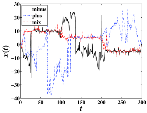
Figure 2: (Color online) Comparison of the three lead-lag thermal optimal paths using the three distances $\epsilon_{-}$ or $\epsilon_{+}$, and $\epsilon_{\pm}$. The temperature is $T=0.1$.

Figure 3 tests the robustness of the reconstructed lead-lag path using the distance $\epsilon_{\pm}$ with respect to different choices of the temperature: $T=1$, $0.2$, $0.1$, and $0.01$. Recall that a vanishing temperature corresponds to selecting the lead-lag path which has the minimum total sum of distances along its length. At the opposite, a very large temperature corresponds to wash out the information contained in the distance matrix and treat all paths on the same footing. In between, a finite temperature allows us to average the contribution over neightboring paths with similar energies, making the estimated lead-lag path more robust to noise-like structures in the distance matrix due to noises decorating the two time series. It is apparent that a too small temperature $T=0.01$ leads to spurious large spiky fluctuations around the correct solution. A too large temperature $T=1$ selects a thermally-averaged path which deviates from the correct solution, here mostly at the beginning of the time series. It seems that there is an optimal range of temperatures around $T=0.1-0.2$ for which the correct solution is retrieved with minimal fluctuations around it. The existence of an optimal range of temperature is confirmed in the inset of Figure 3, which shows the root-mean-square (rms) deviations between the reconstructed lead-lag path and the exact solution ($x(t)=+10$ for $1\leq t\leq 100$, $x(t)=+5$ for $101\leq t\leq 200$ and $x(t)=-5$ for $201\leq t\leq 300$) as a function of temperature in the range $0.01\leq T\leq 10$. The existence of a well-defined optimal range of temperatures is strongest for smaller signal-to-noise ratios $f\triangleq\sigma_{\xi}/\sigma_{\eta}$. For large $f$ (weak noise), we observe that smaller temperatures are better, as expected.

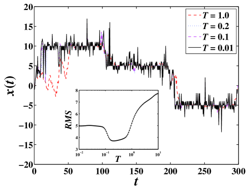
Figure 3: (Color online) Thermally-averaged lead-lag paths of the model (8) for four different temperatures. Inset: root-mean-square (rms) deviations between the reconstructed lead-lag path and the exact solution ($x(t)=+10$ for $1\leq t\leq 100$, $x(t)=+5$ for $101\leq t\leq 200$ and $x(t)=-5$ for $201\leq t\leq 300$) as a function of temperature in the range $0.01\leq T\leq 10$.

The whole purpose of the new distance $\epsilon_{\pm}$ is to be able to identify, not only the lead-lag structure better but also, the existence of possible negative correlations as well as changes of the sign of the correlation with time. We identify the sign $s(t,x(t))=s(t_{1},t_{2})$ of the cross-correlation of the two time series at the times $t_{1},t_{2}$ from the value of $\epsilon_{\pm}$: when $\epsilon_{\pm}$ reduces to $\epsilon_{-}$ (resp. $\epsilon_{+}$), we conclude that the correlation is positive (resp. negative). The corresponding algorithm for the sign of the cross-correlations is thus

$$s(t)=s(t_{1},t_{2})=\left\{\begin{array}[]{cc}+1&~{}~{}{\rm{if}}~{}~{}\epsilon_{\pm}=\epsilon_{-}\\ -1&~{}~{}{\rm{if}}~{}~{}\epsilon_{\pm}=\epsilon_{+}\end{array}\right.$$ (10)

Due to the noises on the two time series, $s(t)$ is also noisy. Thus, to obtain a meaningful information on the sign of the cross-correlations, we apply a smoothing algorithm to $s(t)$. For this, we use the Savitzky-Golay filter with a linear function and include 21 points to the left of each time (to ensure causality). The filtered signal $S(t)$ is shown in Fig. 4. The results are quite consistent with the model in which the correlation is negative in the middle period $100<t<200$ and positive otherwise.

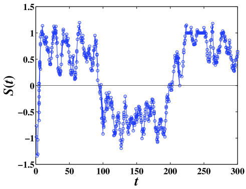
Figure 4: Reconstruction of the sign of the cross-correlation of the model (8,9) by the smoothed sign recognition given by expression (10).

4 Historical volatilities of inflation rate and economic output rate

In this section, we apply our novel technique to the relationship between inflation and real economic output quantified by GDP in the hope of providing new insights. This problem has attracted tremendous interests in past decades in the macroeconomic literature. Different theories have suggested that the impact of inflation on the real economy activity could be either neutral, negative, or positive. Based on the story of Mundell that higher inflation would lower real output [21], Tobin argued that higher inflation causes a shift from money to capital investment and raise output per capita [22], known as the Mundell-Tobin effect. On the contrary, Fischer suggested a negative effect, stating that higher inflation resulted in a shift from money to other assets and reduced the efficiency of transactions in the economy due to higher search costs and lower productivity [23]. In the middle ground, Sidrauski proposed a neutral effect where exogenous time preference fixed the long-run real interest rate and capital intensity [24]. These arguments are based on the rather restrictive assumption that the Philips curve (inverse relationship between inflation and unemployment), taken in addition to be linear, is valid. To evaluate which model characterizes better real economic systems, numerous empirical efforts have been performed and the question is still open.

On the other hand, much focus is put on the nexus between inflation and its uncertainty and economic activity. Okun made the hypothesis of a positive correlation between inflation and inflation uncertainty [25]. Furthermore, Friedman argued that an increase in the uncertainty of future inflation reduces the economic efficiency and lowers the real output rate [26], which is verified empirically (see, e.g. [27, 28, 29, 30, 31, 32]). Following the seminal work of Taylor [33], the output-inflation variability trade-off has been tested extensively in the literature, such as in [34, 35, 36, 37, 38], which are based on model specification. Liu and Liu analyzed the relation between the historical volatility of the output and of the inflation rate, using Chinese data from 1992 to 2004 [19]. They found that there is a strong correlation between the two volatilities and, what is more interesting, that the rolling correlation coefficient changes its sign. In the following, we investigate the nexus between the historical volatilities of inflation and output in a model-free manner to test for possible changes of the signs of their cross-correlation structure.

The data sets, which were retrieved from the FRED II database, include monthly consumer price index (CPI) for all urban consumers and seasonally adjusted quarterly gross domestic product (GDP) covering the time period from 1947 to 2005. The annualized rates of inflation rate $r_{\rm{CPI}}$ and economic growth rate $r_{\rm{GDP}}$ were calculated on a quarterly basis from the CPI and GDP respectively. The historical volatility is calculated in a rolling window as

$$\nu(t)=\left[\frac{1}{\Delta{t}}\sum_{s=t-\Delta{t}+1/4}^{t}\left[r(t)-\mu(t)\right]^{2}\right]^{1/2}~{},$$ (11)

where $r=r_{\rm{CPI}}$ for inflation rate and $r=r_{\rm{GDP}}$ for growth rate, and $\mu(t)$ is their corresponding mean in the rolling window $[t-\Delta{t}+1/4,t]$. The unit of $t$ and $\Delta{t}$ is one year. The resulting historical volatility series $\nu_{\rm{CPI}}(t)$ and $\nu_{\rm{GPD}}(t)$ are shown in the upper panel of Fig. 5 for the time period $[1950,1960]$, with $\Delta{t}=3$ years. Since the volatility $\nu(t)$ is non-stationary (as shown by a standard unit-root test), we use the first-difference of volatility $\Delta{\nu}(t)$, shown in the lower panel of Fig. 5. We focus on the 10-year time period $[1950,1960]$ only for a clearer visualization since the analysis and results are the same qualitatively in other time periods.

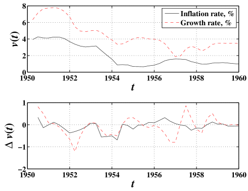
Figure 5: Upper panel: quarterly historical volatilities of the annualized inflation rate and economic growth rate of the United States of America; lower panel: their quarterly changes.

Visual inspection of the lower panel of Fig. 5 suggests that the variations of the volatilities $\nu_{\rm{CPI}}(t)$ and $\nu_{\rm{GPD}}(t)$ are approximately synchronous from 1951 to 1954 and then become approximately anti-phased from 1955 to 1958. Can this be confirmed or falsified by the technique proposed here? To address this question, we determine the smoothed sign function $S(t)$ determined as explained at the end of the previous section. Our tests show that the lead-lag path is close to the diagonal and that there is no significant gain obtained by allowing for a time-varying lag between the variations of the volatilities $\nu_{\rm{CPI}}(t)$ and $\nu_{\rm{GPD}}(t)$. We thus calculate $S(t)$ by smoothing the signal $s(t)$ defined by (10) with the distance matrix constructed using definition (3) along the diagonal of the plane $(t_{1},t_{2})$ (in other words, for $x(t)=0$). We again use the causal Savitzky-Golay filter with a quadratic polynomial and $N_{L}$ data points to the left of each time step $t$ plus the point at $t$ itself. As shown in Fig. 6, we find that the sign signal function $S(t)$ is quite robust with respect to variations of the smoothing parameter $N_{L}$ in the range $N_{L}=5-15$. For comparison, we also plot in Fig. 6 the cross-correlation function $C(t)$ in rolling windows of three years.

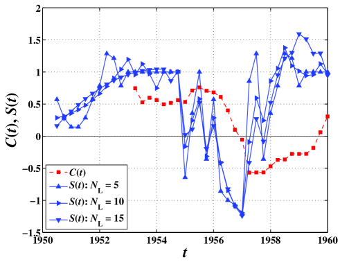
Figure 6: Determination of the sign of the correlation between the variations of the volatilities $\nu_{\rm{CPI}}(t)$ and $\nu_{\rm{GPD}}(t)$ as a function of time in a running window of three years. Our new method $S(t)$ (triangles with three values of the smoothing parameter $N_{L}$) is compared with the cross-correlation $C(t)$ in a running window of size equal to three years (squares).

The reconstructed sign of the correlations between variations of the volatilities $\nu_{\rm{CPI}}(t)$ and $\nu_{\rm{GPD}}(t)$ is in good agreement with and actually makes more precise the visual impression mentioned above. In particular, one can observe that the transition from a synchronicity to anti-phased was gradual with possible ups and downs before the anti-correlation set in in 1956. In contrast, the cross-correlation method suffers from a serious lack of reactivity, predicting a change of correlation sign two years or so after it actually happened. We can thus conclude that our new measure outperforms significantly the traditional cross-correlation measure for real-time identification of switching of correlation structures.

5 Concluding remarks

We have extended the thermal optimal path method [8, 9] in order to, not only identify the time-varying lead-lag structure between two time series but also, to measure the sign of their cross-correlation. In so doing, the identification of the lead-lag structure is improved when there is the possibility for the sign of their correlation to shift. In this goal, the main modification of the method previously introduced in Refs.[8, 9] consists in generalizing the distance matrix in such a way that both correlated and anti-correlated time series can be matched optimally.

A synthetic numerical example has been presented to verify the validity of the new method. Extensive numerical simulations have determined the existence of an optimal range $T\sim(0.1,1)$ of temperatures to use for the robust thermal averaging. We have also proposed a new measure, the sign signal function $S(t)$, that allows us to identify the sign of the correlation structure between two time series.

We have applied our new method to the investigation of possible shifts between synchronous to anti-phased variations of the historical volatility of the USA inflation rate and economic growth rate. The two variables are found positively correlated and in a synchronous state in the 1950’s except over the time period from the last quarter of 1954 till around 1958, when they were in a asynchronous phase (approximately anti-phased). While the traditional cross-correlation function fails to capture this behavior, our new TOP method provides a precise quantification of these regime shifts.

The emphasis of this paper has been methodological. Extensions will investigate the economic meaning of the change of correlation structures as shown here. One possible candidate is the concept of shifts of convention, as discussed in the introduction. More work on many more examples is needed to ascertain the generality of these effects. Overall, the development of better and more precise quantitative tools is progressively unraveling a picture according to which variability and changes of correlation structures is the rule rather than the exceptions in macroeconomics and in financial economics, in the spirit of Aoki and Yoshikawa [39].

Acknowledgments:

We are grateful to M. Wyart for helpful discussions. This work was partially supported by the National Natural Science Foundation of China (Grant No. 70501011), the Fok Ying Tong Education Foundation (Grant No. 101086), and the Alfred Kastler Foundation.

References

- [1] C. W. J. Granger, Testing for causality: A personal viewpoint, J. Econ. Dyn. Control 2 (1980) 329–352.
- [2] R. Ashley, C. W. J. Granger, R. Schmalensee, Advertising and aggregate consumption - an analysis of causality, Econometrica 48 (1980) 1149–1167.
- [3] R. F. Engle, H. White (Eds.), Cointegration, Causality, and Forecasting: A Festschrift in Honour of Clive W.J. Granger, Oxford University Press, Oxford, 1999.
- [4] R. Q. Quiroga, K. T., P. Grassberger, Event synchronization: A simple and fast method to measure synchronicity and time delay patterns, Phys. Rev. E 66 (2002) 041904.
- [5] J.-P. Eckmann, S. Kamphorst, D. Ruelle, Recurrence plots of dynamical systems, Europhys. Lett. 4 (1987) 973–977.
- [6] N. Marwan, J. Kurths, Nonlinear analysis of bivariate data with cross recurrence plots, Phys. Lett. A 302 (2002) 299–307.
- [7] N. Marwan, M. Thiel, N. Nowaczyk, Cross recurrence plot based synchronization of time series, Nonlin. Processes Geophys. 9 (2002) 325–331.
- [8] D. Sornette, W.-X. Zhou, Non-parametric determination of real-time lag structure between two time series: the “optimal thermal causal path” method, Quant. Finance 5 (2005) 577–591.
- [9] W.-X. Zhou, D. Sornette, Non-parametric determination of real-time lag structure between two time series: The “optimal thermal causal path” method with application to economic data, J. Macroeconomics 28 (2006) 197–226.
- [10] J. M. Keynes, The General Theory of Employment, Interest and Money, McMillan, London, 1936.
- [11] A. Orléan, Le rôle des conventions dans la logique monétaire, in Salais R. et L. Thévenot, eds. Le travail. Marchés, règles, conventions, Economica-INSEE (1986) 219–238.
- [12] A. Orléan, Anticipations et conventions en situation d’incertitude, Cahiers d’Economie Politique 13 (1987) 153–172.
- [13] A. Orléan, Pour une approche cognitive des conventions économiques, Revue Economique 40 (1989) 241–272.
- [14] A. Orléan, How do conventions evolve?, J. Evolutionary Econ. 2 (1992) 165–177.
- [15] A. Orléan, L’économie des conventions: définitions et résultats, in: A. Orléan (Ed.), Analyse économique des Conventions, Presses Universitaires de France, coll. “Quadrige”, Paris, 2004.
- [16] R. Boyer, A. Orléan, Persistance et changement des conventions. Deux modèles simples et quelques illustrations, in: A. Orléan (Ed.), Analyse économique des Conventions, 2nd Edition, Presses Universitaires de France, coll. “Quadrige”, Paris, 2004.
- [17] A. Orléan, Efficience, finance comportementaliste et convention : une synthèse théorique, in Boyer R., Dehove M. and D. Plihon, Les crises financières, Rapport du Conseil d’Analyse Economique, Oct. Compléments A (2004) 241–270.
- [18] M. Wyart, J.-P. Bouchaud, Self-referential behaviour, overreaction and conventions in financial markets, J. Econ. Behav. Org. (2006) in press.
- [19] J.-Q. Liu, Z.-G. Liu, The analysis of dynamic patterns and resources of output volatilities in China’s business cycles, Economic Research Journal (Chinese) 40 (3) (2005) 26–35.
- [20] X.-H. Wang, S. Havlin, M. Schwartz, Directed polymers at finite temperatures in 1+1 and 2+1 dimensions, J. Phys. Chem. B 104 (2000) 3875–3880.
- [21] R. A. Mundell, Inflation and real interest, J. Polit. Econ. 71 (1963) 280–283.
- [22] J. Tobin, Money and economic growth, Econometrica 33 (1965) 671–684.
- [23] S. Fischer, Money and production function, Econ. Inq. 12 (1974) 517 C533.
- [24] M. Sidrauski, Rational choice and patterns of growth in a monetary economy, Am. Econ. Rev. 57 (1967) 534–544.
- [25] A. M. Okun, The mirage of economic inflation, Brookings Papers Econ. Activity 1971 (2) (1971) 485–498.
- [26] M. Friedman, Nobel lecture: Inflation and unemployment, J. Polit. Econ. 85 (1977) 451–472.
- [27] G. K. Davis, B. Kanago, On measuring the effect of inflation uncertainty on real GNP growth, Oxford Econ. Papers 48 (1996) 163–175.
- [28] G. K. Davis, B. Kanago, High and uncertain inflation: Results from a new data set , Journal of Money, Credit, and Banking 30 (1998) 218–230.
- [29] F. Al-Marhubi, Cross-country evidence on the link between inflation volatility and growth, Appl. Econ. 30 (1998) 1317–1326.
- [30] K. B. Grier, M. J. Perry, The effects of real and nominal uncertainty on inflation and output growth: Some GARCH-M evidence, J. Appl. Economet. 15 (2000) 45–58.
- [31] M. D. Hayford, Inflation uncertainty, unemployment uncertainty and economic activity, J. Macroeconomics 22 (2000) 315–329.
- [32] S. Fountas, M. Karanasos, J. Kim, Inflation uncertainty, output growth uncertainty and macroeconomic performance, Oxford Bulletin Econ. Stat. 68 (2006) 319–343.
- [33] J. B. Taylor, Estimation and control of a macroeconomic model with rational expectations, Econometrica 47 (1979) 1267–1286.
- [34] R. H. Defina, T. C. Stark, H. E. Taylor, The long-run variance of output and inflation under alternative monetary policy rules, J. Macroeconomics 18 (1996) 235–251.
- [35] J. C. Fuhrer, Inflation/output variance trade-offs and optimal monetary policy, Journal of Money, Credit, and Banking 29 (1997) 214–234.
- [36] D. Cobham, P. Macmillan, D. G. Mcmillan, The inflation/output variability trade-off: Further evidence, Appl. Econ. Lett. 11 (2004) 347–350.
- [37] J. Lee, The inflation-output variability tradeoff and monetary policy: Evidence from a GARCH model, Southern Econ. J. 69 (2002) 175–188.
- [38] J. Lee, The inflation-output variability trade-off: OECD evidence, Contemp. Econ. Pol. 22 (2004) 344–356.
- [39] M. Aoki, H. Yoshikawa, Reconstructing Macroeconomics: A Perspective from Statistical Physics and Combinatorial Stochastic Processes, Cambridge University Press, Cambridge, 2006.