First-order strong field approximation for high-order harmonic generation

Abstract

Recently it was shown [A. Gordon and F. X. Kärtner, Phys. Rev. Lett. 95, 223901 (2005)] that the strong field approximation (SFA) for high-order harmonic generation (HHG) is significantly improved when the SFA wave function is used with the acceleration rather than the length form of the dipole operator. In this work it is shown that using the acceleration form upgrades the SFA from zeroth-order to first-order accuracy in the binding potential. The first-order correct three-step model ($\rm 1^{st}$-order TSM) obtained thereby is systematically compared to its standard zeroth-order counterpart ($\rm 0^{th}$-order TSM) and it is found that they differ significantly even for energetic electrons. For molecules (in the single-electron approximation), the $\rm 0^{th}$-order and the $\rm 1^{st}$-order TSMs in general disagree about the connection between the orbital symmetry and the positions of the minima in the HHG spectrum. At last, we briefly comment on gauge and translation invariance issues of the SFA.

I Introduction

The strong field approximation (SFA) Keldysh ; Faisal ; Reiss is a key technique in the study of interactions of matter with intense laser fields. In particular, the SFA is used to describe high-order harmonic generation (HHG) Becker89 ; Corkum ; Lewenstein ; IvanovBrabec . The three-step model (TSM) Corkum ; Lewenstein ; IvanovBrabec , which is based on the SFA, has proven very successful describing much of the experimental behavior. The best known examples are the cutoff formula Corkum ; Lewenstein ; IvanovBrabec and time-frequency structure of the HHG signal Salieres , which led to the prediction of attosecond pulses atto . Reviews can be found in Refs. BrabecReview ; KnightReview .

It has been long known however that the TSM is incorrect by 1-2 orders of magnitude predicting the spectral intensity of HHG in atomic hydrogen, as found from comparisons with numerically-exact results Tempea ; BrabecReview . For the $\rm H_{2}^{+}$ ion the TSM gives a spectrum which is many orders of magnitude away from numerically-exact results GKPRL , and the shape of the spectrum can be heavily distorted GKPRL ; Bandrauk1 .

HHG experiments are now coming to the point where more accurate theory is needed. The race towards harnessing HHG for a coherent short wavelength source KrauszWaterWindow ; Murnane1997 ; KrauszNature05 can benefit from quantitative theoretical estimates of the HHG efficiency, which to date are very scarce BrabecEffi . The recent orbital imaging experiment CorkumNature uses the HHG spectrum to infer the structure of a molecular orbital, which also requires quantitatively reliable theory, capable of giving a precise description of the shape of the HHG spectrum.

In a recent theoretical work GKPRL we proposed a modified version of the TSM, where the SFA wavefunction is used with the dipole operator in the acceleration rather than the length form. Comparison of the TSM with a numerical solution of the time dependent Schrödinger equation (TDSE) then demonstrated excellent quantitative agreement for atomic hydrogen, and significantly improved agreement for the $\rm H_{2}^{+}$ ion. The argument why using the acceleration form improves the TSM so much was that the TSM then becomes correct to first order in the binding potential (we shall henceforth refer to the TSM obtained this way as $\rm 1^{st}$-order TSM), whereas the standard TSM Corkum ; Lewenstein ; IvanovBrabec ($\rm 0^{th}$-order TSM) is correct to zeroth order in the binding potential.

This work is a followup on Ref. GKPRL , and it has three goals. First, the first-order accuracy of the $\rm 1^{st}$-order TSM is established. Second, a detailed and general comparison between the $\rm 1^{st}$-order TSM and the $\rm 0^{th}$-order TSM is given. It is shown that the two always disagree with respect to the connection between the orbital symmetry and the positions of the minima in the HHG spectrum, as demonstrated for $\rm H_{2}^{+}$ GKPRL ; Bandrauk1 . Third, the opportunity of re-deriving the SFA is used to give a perspective on some delicate issues in the derivation, such as gauge and translation invariance, which have been under debate Milonni ; Kopold ; dispute ; BeckerBauerGauge ; ChLe06 .

This paper is organized as follows. In Sections II and III the derivation of the SFA and $\rm 0^{th}$-order TSM is reviewed, in an attempt to illuminate some subtleties in the derivation and in order to set the stage for deriving the $\rm 1^{st}$-order TSM in Sec. IV. Section V compares the $\rm 0^{th}$-order and $\rm 1^{st}$-order TSMs, and Sec. VI is dedicated to the discussion of gauge and translation invariance issues in the SFA. Section VII gives a brief summary.

Atomic units are adopted throughout the paper.

II Strong field approximation

This work is restricted to the single-electron approximation, where an atom or a molecule are modeled by an electron in an effective (local) potential $V(\mathbf{r})$:

$$H_{0}=-\frac{\nabla^{2}}{2}+V(\mathbf{r})+I_{p},$$ (1)

$I_{p}$ is the binding energy of the ground state, and is added to Eq. (1) for convenience reasons, such that the ground state of $H_{0}$ has zero energy. The atom or molecule is placed in a linearly polarized electric field $E(t)$. The $x$ axis is chosen along the direction of polarization, the wavelength is assumed sufficiently long such that the dipole approximation holds, and the length gauge is chosen, to give the Hamiltonian

$$H(t)=H_{0}-E(t)x.$$ (2)

The SFA is usually presented [see, e. g. Ref. KnightReview and references therein] as a perturbative expansion in $V(\mathbf{r})$, where the unperturbed Hamiltonian is the Volkov Hamiltonian

$$H_{V}(t)=-\frac{1}{2}\nabla^{2}-E(t)x+I_{p}.$$ (3)

The evolution operator $U_{V}(t,t^{\prime})$ of $H_{V}(t)$, defined by

$$i\partial_{t}U_{V}(t,t^{\prime})=H_{V}(t)U_{V}(t,t^{\prime});\quad U_{V}(t^{\prime},t^{\prime})=\mathbbm{1},$$ (4)

is known exactly Lewenstein . Using the Lippmann-Schwinger equation one can approximate $U(t,t^{\prime})$, the evolution operator associated with $H(t)$ (defined through Eq. (4) with all $V$ subscripts omitted) to arbitrary order in $V(\mathbf{r})$ Milo1 . The zeroth and first order would be

$$U_{0}(t,t^{\prime}) = U_{V}(t,t^{\prime})$$ (5)

$$U_{1}(t,t^{\prime}) = -i\int_{t^{\prime}}^{t}dt^{\prime\prime}U_{V}(t,t^{\prime\prime})VU_{V}(t^{\prime\prime},t^{\prime}).$$ (6)

With the operator $U(t,t^{\prime})$ at hand, any problem can be solved.

If at time $t=0$ the electron is in the ground state $|0\rangle$ of $H_{0}$, the wavefunction $|\psi(t)\rangle$ at any time would be given by

$$|\psi(t)\rangle=U(t,0)|0\rangle.$$ (7)

One therefore could suggest approximating $U(t,t^{\prime})$ in Eq. (7) by the perturbative expansion outlined in Eqs. (5, 6). However this is not the way the SFA is usually performed. The route is rather by making the ansatz Lewenstein

$$|\psi\rangle=a(t)|0\rangle+|\varphi(t)\rangle.$$ (8)

$a(t)$ has the initial conditions $a(0)=1$ and is determined later. In other words, the way we split $|\psi\rangle$ into $a(t)|0\rangle$ and $|\varphi(t)\rangle$ is not yet defined.

Let now $|\varphi(t)\rangle$ be the exact solution of

$$i|\dot{\varphi}(t)\rangle=H(t)|\varphi(t)\rangle-a(t)E(t)x|0\rangle,$$ (9)

which in terms of $U$ reads

$$|\varphi(t)\rangle=-i\int_{0}^{t}U(t,t^{\prime})E(t^{\prime})xa(t^{\prime})|0\rangle dt^{\prime}.$$ (10)

Let us assume for the moment that $a(t)$ is specified. The SFA approximates $U$ in Eq. (10) by a perturbation series in $V$ upon $U_{V}$.

One can now ask why the SFA approximates $U$ in Eq. (10) rather than in Eq. (7), if both lead to an exact wavefunction when $U$ is exact? In other words, why one needs the ansatz (8) and the rather non-straightforward Eq. (9)? To our understanding, the answer to these questions is that the perturbed $U_{V}(t,t^{\prime})$ is a very bad approximation for describing the evolution of (quasi) bound states.

Without the laser field, perturbation theory for the evolution operator (the Born series) diverges at bound states of the full Hamiltonian Newton . The presence of a laser field may change the situation, since formally there are no bound states at all. We are not in a position to make a rigorous mathematical statement about the convergence of the SFA, but since the ground state remains quasi-bound, one may expect convergence difficulties. Obviously, at least for the the zeroth order theory, $U_{V}(t,t^{\prime})$ itself gives a very bad approximation for the evolution of a quasi-bound state. In fact, in the Keldysh ionization rate Keldysh is found rather indirectly, by calculating the rate at which the norm of the continuum increases, and the rate at which the ground-state decays is inferred solely by conservation of the total norm.

The last term in Eq. (9) is therefore added because we know in advance that we are going to use an approximate propagator, which will give a very bad description for the evolution of the ground state. Yet, Eq. (9) provides a clear route for systematically improving the SFA: $a(t)$ is first assumed to be known, and Eq. (9) is solved to in principle an arbitrary order in $V(\mathbf{r})$. Then $a(t)$ is found by demanding the conservation of norm, or by means of other approximations, as the perturbed $U_{V}(t,t^{\prime})$ alone is not well suited for this purpose. Note that in the limit where $U$ is exact, one easily finds from Eq. (9) and Eq. (8) that $a(t)\equiv 1$.

III Zeroth order TSM

In this section we re-derive the standard $\rm 0^{th}$-order TSM. The main reason is that our slightly different derivation lays the technical foundations for establishing the first order accuracy of the $\rm 1^{st}$-order TSM in Sec. IV.

The $\rm 0^{th}$-order TSM is obtained by simply replacing $U(t,t^{\prime})$ by $U_{V}(t,t^{\prime})$ in Eq. (9). Since $U_{V}(t,t^{\prime})$ is known exactly, the solution can be written in a closed form Lewenstein :

$$\langle{\bf p-A}(t)|\varphi(t)\rangle=\phantom{AAAAAAAAAAAAAAA}$$ (11)

$$=-i\int\limits_{0}^{t}dt^{\prime}a(t^{\prime})E(t^{\prime})\langle{\bf p}-{\bf A}(t^{\prime})|x|0\rangle e^{-iS({\bf p},t,t^{\prime})}.$$ (12)

${\bf A}(t)\equiv-{\bf\hat{x}}\int^{t}E(t^{\prime})dt^{\prime}$ is a vector potential that describes the electric field $E(t)$, and

$$S({\bf p},t,t^{\prime})\equiv\frac{1}{2}\int\limits_{t^{\prime}}^{t}({\bf p}-{\bf A}(t^{\prime\prime}))^{2}dt^{\prime\prime}+I_{p}(t-t^{\prime}).$$ (13)

At this point we slightly deviate from the standard derivation of the TSM Lewenstein ; IvanovBrabec : We perform the saddle-point integration in Eq. (11) right now, before proceeding. This calculation was pioneered by Keldysh Keldysh and is further discussed in a vast number of SFA studies [see e. g. Ref. DeloneKrainov and references therein]. The discussion in this work is limited to the tunneling regime, which is defined by the requirements DeloneKrainov :

$$E_{0} \ll (2I_{p})^{3/2}$$ (14a)

$$\gamma\equiv\frac{\omega}{E_{0}}\sqrt{2I_{p}} \ll 1$$ (14b)

$$\omega \ll I_{p}$$ (14c)

In Eq. (14a) $E_{0}$ is the amplitude of the driving field and $\omega$ is its frequency. These parameters are precisely defined for a sinusoidal driving field, and more loosely for a general field, such as a sinusoidal field with an envelope. In the latter case, $\omega$ can be thought of as the parameter characterizing the timescale over which $E(t)$ varies. $\gamma$ is the well known Keldysh parameter Keldysh . Note that the requirement (14c) follows from (14a) and (14b).

Under the conditions (14), the saddle-point integration of Eq. (11) is carried out to give

$${\langle{\bf p-A}(t)|\varphi(t)\rangle}=\frac{\sqrt[4]{2I_{p}}}{\sqrt{\pi}}\sum_{n}a(t_{n}(p_{x}))\frac{w((E(t_{n}(p_{x}))}{|E(t_{n}(p_{x}))|}\times$$ (15)

$$\times e^{\frac{-p_{\perp}^{2}}{|E(t_{n}(p_{x}))|\sqrt{2I_{p}}}}e^{-iS(\mathbf{p},t,t_{n}(p_{x}))}.\phantom{A}$$ (16)

$w(E)$ is the static Stark ionization rate associated with the ground state, $p_{\perp}^{2}\equiv p_{y}^{2}+p_{z}^{2}$, and the function $t_{n}(p_{x})$ is the set of positive real solutions of the equation

$$p_{x}=A_{x}(t_{n}(p_{x})).$$ (17)

The number of solutions depends on $E(t)$. $a(t)$ can now be found by requiring conservation of the norm in Eq. (8) [neglecting $\langle 0|\varphi(t)\rangle$] to give the well-known expression BrabecReview

$$|a(t)|^{2}=e^{-\int_{0}^{t}w(E(t^{\prime}))dt^{\prime}}.$$ (18)

Using the ansatz (8) with the wavefunction (15), one can now compute the expectation value of the dipole moment:

$$\langle x\rangle = |a(t)|^{2}\langle 0|x|0\rangle+\langle\varphi(t)|x|\varphi(t)\rangle+\xi_{0}(t)+\xi_{0}^{*}(t),\phantom{AA}$$ (19)

where

$$\xi_{0}(t)\equiv a^{*}(t)\langle 0|x|\varphi(t)\rangle.$$ (20)

The origin of coordinates can always be chosen such that the first term in Eq. (19) vanishes. The second term has no high harmonics IvanovRza , since matrix elements of $x$ between two different Volkov states vanish. The high harmonics come from the cross term $\xi_{0}(t)$. Using Eq. (15) we find:

$$\xi_{0}(t)=a^{*}(t)\frac{\sqrt[4]{2I_{p}}}{\sqrt{\pi}}\sum_{n}\int d^{3}p\langle 0|x|{\bf p-A}(t)\rangle a(t_{n}(p_{x}))\times$$ (21)

$$\times\frac{w((E(t_{n}(p_{x}))}{|E(t_{n}(p_{x}))|}e^{\frac{-p_{\perp}^{2}}{|E(t_{n}(p_{x}))|\sqrt{2I_{p}}}}e^{-iS(\mathbf{p},t,t_{n}(p_{x}))}\phantom{A}$$ (22)

The $\mathbf{p}$ integration is now carried out in the stationary phase approximation as in Ref. Lewenstein . The stationary phase is attained at $p_{\perp}=0$ and at all $p_{x}$ values such that $t_{n}(p_{x})$ satisfy [see Appendix A for a more careful discussion]

$$\int_{t_{n}}^{t}(A(t_{n})-A(t^{\prime\prime}))dt^{\prime\prime}=0.$$ (23)

For any given $t$, $\bar{t}_{n}(t)$ is defined as the set of solutions to Eq. (23), i. e. birth times of trajectories that end up at the origin at time $t$. Then in the stationary phase approximation Eq. (21) gives

$$\xi_{0}(t) = e^{\frac{-i\pi}{4}}\sqrt[4]{2I_{p}}2^{3/2}\pi\sum_{n}\frac{e^{-i\overline{S}_{n}(t)}}{(t-\overline{t}_{n}(t))^{3/2}}a^{*}(t)\times$$ (24)

$$\times a(\overline{t}_{n}(t))\langle 0|x|\mathbf{A}(\overline{t}_{n}(t))-\mathbf{A}(t)\rangle\frac{w((E(\bar{t}_{n}(t))}{|E(\bar{t}_{n}(t))|},\phantom{AA}$$ (25)

where $\bar{S}_{n}(t)\equiv S(\mathbf{A}(\bar{t}_{n}(t)),t,\bar{t}_{n}(t))$.

Eq. (24) is identical to the original TSM expression derived in Ref. IvanovBrabec . The only difference is that Eq. (24) takes into account the depletion of the ground state, and that all numerical prefactors ($2^{3/2}\pi$) were calculated. The re-derivation of the $\rm 0^{th}$-order TSM is now concluded.

IV First order TSM

A straight forward way to upgrade the TSM from zeroth to first order accuracy in $V$ would be improving the TSM wavefunction (11) by adding the first-order correction to the evolution operator, Eq. (6). This method has been employed in Ref. Lew95 , for improving the SFA theoretical description of above threshold ionization. For HHG we propose another method, which is significantly simpler, and does not require correcting the wavefunction.

If $|\psi(t)\rangle$ is the exact solution of the time-dependent Schrödinger equation with the Hamiltonian (2), then the Ehrenfest theorem holds:

$$\frac{d^{2}\langle\psi(t)|x|\psi(t)\rangle}{dt^{2}}=$$ (26a)

$$= \frac{d\langle\psi(t)|p_{x}|\psi(t)\rangle}{dt}=$$ (26b)

$$= -\langle\psi(t)|\partial_{x}V(\mathbf{r})|\psi(t)\rangle+E(t)$$ (26c)

Therefore computing the time-dependent dipole expectation value in all three forms of Eq. (26), length (26a), velocity (26b), or acceleration (26c), is equivalent if accompanied by the appropriate differentiation or integration in time.

However with the approximate wavefunction given by Eqs. (8) and (15), the results will be in general different for each form. One therefore has to make a choice which form to use for this particular wavefunction. We argue that the acceleration form gives in general the best results, since even if $|\varphi(t)\rangle$ is only correct to zeroth order in $V(\mathbf{r})$, the expectation value is automatically correct, at least formally, to first order in $V(\mathbf{r})$. One therefore needs to evaluate

$$\frac{d^{2}\langle x\rangle}{dt^{2}} = \ddot{\xi}_{1}(t)+\ddot{\xi}^{*}_{1}(t)+\ddot{\xi}_{c}(t)$$ (27)

where

$$\ddot{\xi}_{1}(t) \equiv -a^{*}(t)\langle 0|\partial_{x}V(\mathbf{r})|\varphi(t)\rangle$$ (28)

$$\ddot{\xi}_{c}(t) \equiv -\langle\varphi(t)|\partial_{x}V(\mathbf{r})|\varphi(t)\rangle$$ (29)

The last term of Eq. (26c) has been dropped, since it is the driving field itself and thus contains no harmonics. It is easy to show, exploiting the commutator $[p,H_{0}]$, that $\langle 0|\partial_{x}V(\mathbf{r})|0\rangle=0$ [irrespectively of the position of origin], which is why the corresponding term in Eq. (27) is missing.

Note that the mere appearance of $V$ in Eq. (27) is not sufficient to warrant first order accuracy. One can see that, for example, from the fact that zeroth order SFA expressions in $V$ can be transformed such that they appear linear or quadratic in $V$ Lohr ; BeckerLew . The (formal) first-order accuracy of Eq. (27) is established by the fact that a first-order correction in $V$ to the wavefunction in Eq. (11) will result in only a second order correction in $V$ in Eq. (27). This is why we dedicated Sec. II to carefully defining the procedure by which the SFA is corrected order by order in $V$.

The cross term $\ddot{\xi}_{1}$ has the same structure as $\xi_{0}$ [Eq. (20)]. Going through the same steps that have led to Eq. (24), one arrives at the same expression $\ddot{\xi}_{1}$, with the only difference that the matrix element $\langle 0|x|\mathbf{k}\rangle$ is replaced by $-\langle 0|\partial_{x}V(\mathbf{r})|\mathbf{k}\rangle$:

$$\ddot{\xi}_{1}(t) = -e^{\frac{-i\pi}{4}}\sqrt[4]{2I_{p}}2^{3/2}\pi\sum_{n}\frac{e^{-i\overline{S}_{n}(t)}}{(t-\overline{t}_{n}(t))^{3/2}}\times$$ (30)

$$\times a^{*}(t)a(\overline{t}_{n}(t))\frac{w((E(\bar{t}_{n}(t))}{|E(\bar{t}_{n}(t))|}$$ (31)

$$\times \langle 0|\partial_{x}V(\mathbf{r})|\mathbf{A}(\overline{t}_{n}(t))-\mathbf{A}(t)\rangle.\phantom{AA}$$ (32)

Eq. (30) is the improved version of the TSM presented in Ref. GKPRL . The change in the expression compared to Eq. (24) is very small and easy to implement, and yet results in a very large difference, especially in the case of molecules.

Eq. (30) is an expression for $\ddot{\xi}_{1}$, but Eq. (27) contains also $\xi_{c}$. It turns out that the contribution of $\ddot{\xi}_{c}$ to HHG is smaller by at least $O(\omega^{3/2})$ than that of $\ddot{\xi}_{1}$. $\ddot{\xi}_{c}$ is therefore negligible for $\omega\ll 1$, which coincides with Eq. (14c) when $I_{p}$ is of $O(1)$. The latter holds for all neutral (or not highly charged) atoms and molecules. The evaluation of $\ddot{\xi}_{c}$ is rather lengthy, especially for potentials with a long-ranged Coulomb tail, and is given in Appendix B.

V $\bf 0^{th}$ vs. $\bf 1^{st}$-order TSM – comparison

The $\rm 0^{th}$-order TSM suggests Eq. (20) as an approximation to the dipole moment, whereas the $\rm 1^{st}$-order TSM suggests Eq. (28). In order to compare them conveniently, we now differentiate Eq. (20) twice in time and compare $\ddot{\xi}_{0}$ with $\ddot{\xi}_{1}$. This is done in detail in Appendix C. The result is that under the condition (14a), in order to obtain $\ddot{\xi}_{0}(t)$, one has to replace the $\rm 1^{st}$-order TSM recombination amplitude

$$a_{\rm rec}^{\rm new}(\mathbf{k})=\langle 0|\partial_{x}V(\mathbf{r})|\mathbf{k}\rangle,$$ (33)

in Eq. (28) by

$$a_{\rm rec}^{\rm old}(\mathbf{k})=(I_{p}+\tfrac{1}{2}|\mathbf{k}|^{2})^{2}\langle 0|x|\mathbf{k}\rangle.$$ (34)

Comparing the $\rm 1^{st}$-order TSM and the $\rm 0^{th}$-order TSM is thus reduced to comparing $a_{\rm rec}^{\rm new}$ and $a_{\rm rec}^{\rm old}$ respectively.

The two expressions look different, and indeed they are. A detailed comparison requires the knowledge of $V$. However in order to gain some general insight, in what follows we study the $k\to\infty$ asymptotic behavior of $a_{\rm rec}^{\rm new}$ and $a_{\rm rec}^{\rm old}$. Some pretty general statements can be made about $k\to\infty$, which turn out to provide important insights also for $k$-s of $O(1)$.

V.1 High-momentum asymptotic evaluation

$a_{\rm rec}^{\rm old}(\mathbf{k})$ can be written as

$$a_{\rm rec}^{\rm old}(\mathbf{k})=\frac{1}{(2\pi)^{3/2}}\int\chi^{\rm old}(\mathbf{r})e^{-i\mathbf{k}\cdot\mathbf{r}}dr$$ (35)

(and similarly for $a_{\rm rec}^{\rm new}(\mathbf{k})$ and $\chi^{\rm new}(\mathbf{r})$), where

$$\chi^{\rm old}(\mathbf{r}) \equiv (I_{p}-\tfrac{1}{2}\nabla^{2})^{2}x\psi_{0}(\mathbf{r})$$ (36)

$$\chi^{\rm new}(\mathbf{r}) \equiv \psi_{0}(\mathbf{r})\partial_{x}V(\mathbf{r}),$$ (37)

with $\psi_{0}(\mathbf{r})\equiv\langle\mathbf{r}|0\rangle$. Using $H_{0}|0\rangle=0$, Eq. (36) can be transformed into

$$\chi^{\rm old}(\mathbf{r}) = 2\psi_{0}(\mathbf{r})\partial_{x}V(\mathbf{r})+2V(\mathbf{r})\partial_{x}\psi_{0}(\mathbf{r})$$ (38)

$$+ xV^{2}(\mathbf{r})\psi_{0}(\mathbf{r})+x\nabla V(\mathbf{r})\cdot\nabla\psi_{0}(\mathbf{r})+$$ (39)

$$+ \tfrac{1}{2}x\psi_{0}(\mathbf{r})\nabla^{2}V(\mathbf{r})$$ (40)

The $k\to\infty$ asymptotic behavior of $a_{\rm rec}^{\rm old}(\mathbf{k})$ and $a_{\rm rec}^{\rm new}(\mathbf{k})$ is dictated by the most singular part $\chi^{\rm old}(\mathbf{r})$ and $\chi^{\rm new}(\mathbf{r})$ respectively, since they are connected by a Fourier transform Simon_Reed .

We now assume that $V(\mathbf{r})$ is an effective potential that represents a molecule (or, as a special case, an atom) with nuclei at positions $\mathbf{r}_{j}$ with charges $Z_{j}$, $j=1...N$. Common choices for an effective potential to model such a system have a $Z_{j}/|\mathbf{r}-\mathbf{r}_{j}|$ singularity near the $j$-th nucleus, which is partially screened off away from the nucleus. Then the last term in Eq. (38) can be written as

$$\tfrac{1}{2}x\psi_{0}(\mathbf{r})\nabla^{2}V(\mathbf{r})=-2\pi x\psi_{0}(\mathbf{r})\sum_{j}Z_{j}\delta(\mathbf{r}-\mathbf{r}_{j})$$ (41)

Now one has to distinguish two cases. The first case is a molecule. Whenever there is more than one nucleus, Eq. (41) does not vanish [apart from possibly a very few orientations of the molecule]. Then the term in Eq. (41) is the most singular one among all terms on the right hand side of Eq. (38), and thus governs $a_{\rm rec}^{\rm old}(\mathbf{k})$ at $k\to\infty$. In this case

$$\chi^{\rm old}(\mathbf{r})\sim-2\pi\sum_{j}x_{j}\psi_{0}(\mathbf{r}_{j})Z_{j}\delta(\mathbf{r}-\mathbf{r}_{j})$$ (42)

where the notation ‘$\sim$’ means ‘equal in its most singular part’.

The second case is an atom, which has only one nucleus, whose position can be always chosen at $\mathbf{r}=0$ [see Sec. VI for a discussion about translation invariance]. In this case Eq. (41) obviously vanishes. Then the most singular term on the right hand side of Eq. (38) is the first one, and we find that

$$\chi^{\rm old}(\mathbf{r})\sim 2\chi^{\rm new}(\mathbf{r})$$ (43)

V.2 Atoms

Eq. (43) implies that for atoms

$$a_{\rm rec}^{\rm old}(\mathbf{k})\to 2a_{\rm rec}^{\rm new}(\mathbf{k}),$$ (44)

where ‘$\to$’ denotes ‘approaches asymptotically at $k\to\infty$’. Thus $a_{\rm rec}^{\rm new}(\mathbf{k})$ and $a_{\rm rec}^{\rm old}(\mathbf{k})$ do not agree even asymptotically for $k\to\infty$, the limit were plane waves approximate the exact continuum states increasingly well. For atoms, the $\rm 0^{th}$-order TSM predicts a 4 times larger HHG yield than the ($\rm 1^{st}$-order TSM). For a $Z/r$ singularity in the potential, the asymptotic behavior of $a_{\rm rec}^{\rm new}$ can be easily worked out to give

$$a_{\rm rec}^{\rm new}(\mathbf{k})\to{\rm i}Z\psi_{0}(0)\sqrt{\frac{2}{\pi}}\frac{k_{x}}{k^{2}}$$ (45)

When $\psi_{0}(0)$ vanishes Eq. (45) is modified.

For finite $k$ the disagreement between $a_{\rm rec}^{\rm new}(\mathbf{k})$ and $a_{\rm rec}^{\rm old}(\mathbf{k})$ can be even greater. For the hydrogen atom one finds GSKPRA

$$a_{\rm rec}^{\rm new}(k_{x}) = \frac{i\sqrt{2}}{\pi}\frac{k_{x}-\tan^{-1}k_{x}}{k_{x}^{2}}$$ (46)

$$a_{\rm rec}^{\rm old}(k_{x}) = \frac{i2^{3/2}}{\pi}\frac{k_{x}}{1+k_{x}^{2}}$$ (47)

for $\mathbf{k}$ lying along the $x$ axis. Fig. 1 compares the two expressions in Eq. (46).

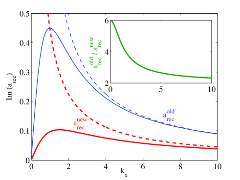
Figure 1: comparison of $a_{\rm rec}^{\rm new}$ [thick red lines] and $a_{\rm rec}^{\rm old}$ [thin blue lines] for hydrogen. The continuous lines correspond to the two expressions in Eq. (46). The dashed lines are the asymptotic expressions [Eq. (44) and Eq. (45)]. The inset shows the ratio between the two expressions in Eq. (46).

V.3 Molecules

The differences between the $\rm 0^{th}$-order TSM and the $\rm 1^{st}$-order TSM for molecules is particularly striking. The two models give opposite relations between orbital symmetry and the positions of the minima in the HHG spectrum, a subject of many recent theoretical and experimental studies Lin ; Marangos1 ; Kanai ; Chang ; Nalda ; Lein2002 ; Knight . A set of minima is predicted by the $\rm 0^{th}$-order TSM with an odd orbital, corresponds to an even orbital in the $\rm 1^{st}$-order TSM, and vice versa.

From Eq. (42) we find that for molecules

$$a_{\rm rec}^{\rm old}(\mathbf{k})\to-\frac{1}{\sqrt{2\pi}}\sum_{j}x_{j}\psi_{0}(\mathbf{r}_{j})Z_{j}e^{-{\rm i}\mathbf{k}\cdot\mathbf{r}_{j}},$$ (48)

whereas from Eq. (33) and Eq. (45) we find

$$a_{\rm rec}^{\rm new}(\mathbf{k})\to{\rm i}\sqrt{\frac{2}{\pi}}\frac{k_{x}}{k^{2}}\sum_{j}\psi_{0}(\mathbf{r}_{j})Z_{j}e^{-{\rm i}\mathbf{k}\cdot\mathbf{r}_{j}},$$ (49)

Observing Eq. (48) and Eq. (49), it becomes clear why the $\rm 0^{th}$-order TSM and $\rm 1^{st}$-order TSM disagree about the connection between the symmetry $\psi_{0}$ and the zeros (or minima) of $|a_{\rm rec}|$. Apart from the additional $k_{x}/k^{2}$ envelope in Eq. (49), which does not affect the position of the zeros, Eq. (49) is the Fourier transform of $x\psi_{0}(\mathbf{r})$, whereas Eq. (48) is the Fourier transform of $\psi_{0}(\mathbf{r})$ (both sampled at the singular points). $x\psi_{0}(\mathbf{r})$ and $\psi_{0}(\mathbf{r})$ obviously have the opposite symmetry with respect to a $x\to-x$ reflection.

In order to illustrate this we consider the $\rm H_{2}^{+}$ ion, where the nuclei are positioned along the $x$ axis, at $x=\pm R/2$. In this case Eq. (48) gives

$$a_{\rm rec}^{\rm old}(\mathbf{k})\to\frac{{\rm i}RC}{\sqrt{2\pi}}\sin(\tfrac{1}{2}k_{x}R),$$ (50)

where $C\equiv\psi_{0}(-\frac{1}{2}R\mathbf{\hat{x}})=\psi_{0}(\frac{1}{2}R\mathbf{\hat{x}})$. In contrast, Eq. (49) gives

$$a_{\rm rec}^{\rm new}(\mathbf{k})\to{\rm i}\sqrt{\frac{2}{\pi}}\frac{k_{x}}{k^{2}}2C\cos(\tfrac{1}{2}k_{x}R),$$ (51)

A zero of $a_{\rm rec}$ at a given $k_{x}$ corresponds to a minimum in the HHG spectral intensity at the frequency $I_{p}+\frac{1}{2}k_{x}^{2}$. The $\rm 0^{th}$-order TSM therefore predicts minima at energies given by $I_{p}+(2\pi n/R)^{2}$ ($n$ is an integer), whereas the $\rm 1^{st}$-order TSM predicts minima at energies given by $I_{p}+(2\pi(n+\frac{1}{2})/R)^{2}$. The latter condition well agrees with numerically-exact results Knight ; GKPRL .

It is easy to see from Eq. (48) and Eq. (49) that if $\psi_{0}(\mathbf{r})$ were an odd rather than even wavefunction with respect to $x\to-x$, the cosine [sine] in Eq. (50) [Eq. (51)] is replaced by a sine [cosine]. Therefore if the $\rm 0^{th}$-order TSM is used for reconstructing $\psi_{0}(\mathbf{r})$ from the HHG spectrum, it flips the symmetry of $\psi_{0}(\mathbf{r})$ from even to odd and vice versa. This statement is, of course, based only on the $k_{x}\to\infty$ asymptotic behavior of the $a_{\rm rec}$-s. Yet it is interesting to note that for $\rm H_{2}^{+}$, Eq. (50) and Eq. (51) approximate Eq. (33) and Eq. (34) reasonably well for low momenta, as Fig. 2 shows.

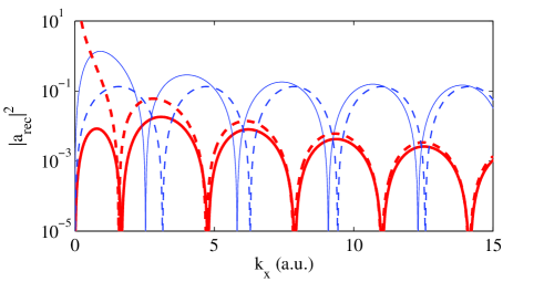
Figure 2: $|a_{\rm rec}^{\rm old}|^{2}$ (thin blue line) and $|a_{\rm rec}^{\rm new}|^{2}$ (thick red line) as function of $v_{x}$ for $\rm H_{2}^{+}$ (R=2). The dashed lines are the corresponding asymptotic ($v_{x}\gg 1$) approximations [Eq. (50) and Eq. (51)].

Note that the $k_{x}/k^{2}$ envelope, which is present in Eq. (49) but absent in Eq. (48), results in an orders-of-magnitude difference in the magnitudes of the $a_{\rm rec}$-s, in addition to the distorted shape.

VI Gauge and translation invariance issues

The dependence of the SFA on gauge has been the subject of lively discussions Reiss ; Milonni ; dispute ; BeckerBauerGauge ; Kopold ; ChLe06 . Here we do not attempt a comprehensive discussion of this subject. However since some steps in Sec. V seem to rely on placing the origin of the laser potential and the atom at the same point, we briefly address the related issue of translation invariance.

Consider thus the Hamiltonian

$$H(t)=-\frac{1}{2}\nabla^{2}+V(\mathbf{r})-E(t)(x-x_{0})+I_{p}$$ (52)

($x_{0}$ is a constant), which is related to Eq. (2) by a gauge transformation. The exact solution of the TDSE with Eq. (52) obviously gives the same time-dependent expectation values as with Eq. (2). However the SFA can give different results for Eq. (52) and Eq. (2). In particular, the SFA with Eq. (52) can give rise to the generation of even harmonics Kopold , which is an artifact.

There is an obvious way by which this problem can be cured, namely, by replacing the ansatz (8) by

$$|\psi\rangle=a(t)e^{-ix_{0}\int E(t)dt}|0\rangle+|\varphi(t)\rangle.$$ (53)

Substituted Eq. (53) into the TDSE with the Hamiltonian (52), it is easy to convince oneself that the results no longer depend on $x_{0}$. This is because wavefunction (8) undergoes exactly the gauge transformation that connects Eq. (52) to Eq. (2), guaranteeing gauge invariance. The SFA depends on the choice of gauge simply because it crucially depends on the choice of the initial ansatz.

One can now ask how to obtain an ansatz for a given gauge a-priori, without e. g. gauge-transforming Eq. (8), and how to obtain the ansatz (8) itself a-priori. Our answer is that the ansatz should provide the best approximation for the evolution of the quasi-bound ground state, since the (perturbed) Volkov evolution operator cannot do it [see Sec. II].

In the low frequency regime [Eq. (14c)], a good approximation for the evolution of the ground state can be found using the adiabatic theorem adiabatic : It is approximately given by $e^{-i\int\varepsilon(E(t))dt}|\phi(E)\rangle$, where the $|\phi(E)\rangle$ and $\varepsilon(E)$ are the field-dependent ground state wavefunction and energy, defined through the eigenvalue equation

$$\left(-\tfrac{1}{2}\nabla^{2}+V(\mathbf{r})-E(x-x_{0})+I_{p}\right)|\phi(E)\rangle=\varepsilon(E)|\phi(E)\rangle.$$ (54)

The adiabatic theorem holds even though $|\phi(E)\rangle$ becomes a resonance NimrodAdiabatic . If we neglect the Stark shift of the energy, we obtain $\varepsilon(E)=Ex_{0}$. Going further and approximating $|\phi(E)\rangle$ by $|\phi(0)\rangle=|0\rangle$, we obtain exactly the ansatz (53), a-priori, without referring to Eq. (8). In fact, Eq. (8) itself is obtained for $x_{0}=0$.

The discussion can be extended to at least one common gauge, namely the velocity gauge. Then the adiabatic argument would again give a modified ansatz, similar to the one used in Ref. BrabecDipole . It is likely that the differences between the length and velocity gauges reported in Ref. BeckerBauerGauge would then disappear.

VII Discussion

The large discrepancy between the $\rm 0^{th}$-order TSM HHG spectra and numerically-exact calculations has been attributed long ago BrabecReview to the SFA wavefunction being inaccurate. It is often argued that this SFA wavefunction is especially inaccurate for molecules Greene . This work strongly supports these ideas: The length and acceleration forms of the dipole operator used on the same SFA wavefunction are shown to give dramatically different results, especially for molecules. For an exact wavefunction the results would be identical, and thus the large discrepancy is evidence for the inaccuracy of the wavefunction.

Since the wavefunction is so far from being exact, it is especially important to use it properly. In this work we have argued that together with the acceleration form of the dipole, the zeroth-order SFA wavefunction leads to an approximation (the $\rm 1^{st}$-order TSM) with first-order overall accuracy in the binding potential. Since the wavefunction itself is so inaccurate, it can lead to very large errors if used otherwise than in the specially-suited way introduced in this work. The accuracy of the $\rm 1^{st}$-order TSM should be tested in terms of the expectation values it generates and not in terms of the wavefunction itself.

We have shown that the continuum-continuum term in the $\rm 1^{st}$-order TSM is negligible compared to the bound-continuum term. Therefore, the widely-used $\rm 0^{th}$-order TSM is upgraded to first-order accuracy by simply replacing $x$ by $\partial_{x}V(\mathbf{r})$ in the recombination amplitude, which is simple to implement. The $\rm 1^{st}$-order TSM shows excellent agreement with numerically-exact results for atoms GKPRL ; SG06 and good agreement for $\rm H_{2}^{+}$ GKPRL .

The SFA decomposes the wavefunction into a continuum, and a quasi-bound ground state. This is justified, since the strong laser field smears the excited states of the unperturbed system and turns them into a continuum Lewenstein . The dynamics of the continuum is approximated by the Volkov propagator, which can be corrected order by order in the binding potential. The quasi-bound state however should be treated separately.

It should be noted that there could be more than one quasi-bound state. For example, the initial state of the electron can be an excited state of the laser-free Hamiltonian $H_{0}$, a case that was not treated in this work. This is commonly the case in single-electron models of multi-electron atoms. Then the states lying energetically below the initial state are also quasi-bound, and should also be treated separately. One simple way to do that is to project these states out of the SFA wavefunction, as briefly discussed at the end of Ref. SG06 .

Appendix A Complementary remarks on the derivation of the $\rm 0^{th}$-order TSM

Eq. (23) is gives the stationary phase condition only to leading order in $\gamma$. In fact, when $S(\mathbf{p},t,t_{n}(p_{x}))$ is differentiated with respect $p_{x}$ taking Eq. (17) into account, the result is

$$\frac{I_{p}}{E(t_{n})}+\int_{t_{n}}^{t}(A(t_{n})-A(t^{\prime\prime}))dt^{\prime\prime}=0.$$ (55)

The second term in Eq. (55) is of the order of $E_{0}/\omega^{2}$, while the first one is of the order of $I_{p}/E_{0}$. Therefore the first term in Eq. (55) is a second-order correction in $\gamma$ to Eq. (23). It is interesting to note however that the subleading term term is meaningful, since the electron is released by tunneling roughly at the turning point ($x=I_{p}/E$) DeloneKrainov rather than at the origin.

Note that the denominator $(t-\overline{t}_{n}(t))^{3/2}$ in Eq. (24) cannot result in a divergence. If the first term in Eq. (23) is retained, the reason is obvious – the duration of a trajectory is never zero, since it begins and ends at different locations. If the first term in Eq. (23) is neglected, as often happens, one can easily show that trajectories for which $t$ approaches $t_{n}(t)$ can only occur at points where $E(t)=0$, and then $w(E)$ vanishes exponentially. Performing the $t^{\prime}$ integration first thus spares the need for the regularizing parameter $\epsilon$ used in, e. g. Ref. Lewenstein .

Note also that the denominator $(t-\overline{t}_{n}(t))^{3/2}$ is correct only to zeroth order in $\gamma$. The leading correction is obtained if the $e^{-p_{\perp}^{2}/(|E(t_{n}(p_{x}))|\sqrt{2I_{p}}}$ factor in Eq. (21) is included in the Gaussian in integration and if Eq. (17) is taken into account when the second derivative of $S$ with respect to $p_{x}$ is computed.

Appendix B Evaluation of the continuum-continuum term

For completeness, in this Appendix the continuum-continuum term $\ddot{\xi}_{c}(t)$ [Eq. (29)] is evaluated. To this aim we define

$$Q(\mathbf{k})\equiv\frac{1}{(2\pi)^{3/2}}\int d^{3}r[\partial_{x}V(\mathbf{r})]e^{-i\mathbf{k}\cdot\mathbf{r}},$$ (56)

the Fourier transform of the force field derived from the potential $V$. It turns out that a long-range Coulomb behavior of $V$ requires more careful evaluation of $\ddot{\xi}_{c}$ than a short-ranged $V$. Since once $|\varphi(t)\rangle$ is given $\ddot{\xi}_{c}(t)$ is linear in $V$, one can write $V$ as a sum of the pure Coulomb potential plus a short-ranged potential, evaluate each term separately, and sum up the results at the end. In what follows we therefore treat the two cases separately.

B.1 Short-range potentials

In order to keep the expressions from becoming too cluttered, we introduce the notation

$$\tilde{a}(t)\equiv\frac{\sqrt[4]{2I_{p}}}{\sqrt{\pi}}a(t)\frac{w(E(t))}{|E(t)|}$$ (57)

Substituting Eq. (15) in Eq. (29) we obtain

$$\ddot{\xi}_{c}(t) = \sum_{n,n^{\prime}}\int dpdp^{\prime}\tilde{a}^{*}(t_{n^{\prime}}(p^{\prime}_{x}))\tilde{a}(t_{n}(p_{x}))\times$$ (58)

$$\times e^{\frac{-{p^{\prime}}_{\perp}^{2}}{|E(t_{n}(p^{\prime}_{x}))|\sqrt{2I_{p}}}}e^{\frac{-p_{\perp}^{2}}{|E(t_{n}(p_{x}))|\sqrt{2I_{p}}}}\times$$ (59)

$$\times e^{iS(\mathbf{p}^{\prime},t,t_{n^{\prime}}(p^{\prime}_{x}))-iS(\mathbf{p},t,t_{n}(p_{x}))}Q(\mathbf{p}^{\prime}-\mathbf{p})$$ (60)

We now carry out the integration in Eq. (58) in the stationary-phase approximation. To this aim we assume that apart from the exponentials in Eq. (58), the rest of the integrand is slowly varying in $\mathbf{p}$. Here it is where we use the short-range property of $V$, which assures that $Q$ is indeed slowly varying in $\mathbf{p}$.

The stationary phase condition in the six-dimensional $\mathbf{p}$-$\mathbf{p}^{\prime}$ momentum space is identical to the one of the integral (21): $p_{\perp}=p^{\prime}_{\perp}=0$, whereas $p_{x}$ and $p^{\prime}_{x}$ are obtained by finding all solutions $\bar{t}_{n}(t)$ that satisfy Eq. (23) and using Eq. (17) to find the corresponding $p_{x}$-s. The result of the integration is

$$\ddot{\xi}_{c}(t)=(2\pi)^{3/2}\sum_{n,n^{\prime}}\frac{\tilde{a}^{*}(\bar{t}_{n^{\prime}})\tilde{a}(\bar{t}_{n})}{(t-\bar{t}_{n})^{3/2}(t-\bar{t}_{n^{\prime}})^{3/2}}$$ (61)

$$\times e^{i\bar{S}(t,\bar{t}_{n^{\prime}})-i\bar{S}(t,\bar{t}_{n})}Q(\mathbf{A}(t_{n^{\prime}})-\mathbf{A}(t_{n}))),$$ (62)

where the dependence of $\bar{t}_{n}$ on $t$ has been suppressed.

Eq. (61) confirms our claim that $\ddot{\xi}_{c}(t)$ is small compared to $\ddot{\xi}_{1}(t)$. $\ddot{\xi}_{1}(t)$ [Eq. (30)] has only a $(2\pi/(t-\bar{t}_{n}))^{3/2}$ prefactor (which is $O(\omega^{3/2})$), whereas for $\ddot{\xi}_{c}(t)$ it is $O(\omega^{3})$. Moreover, $\xi_{1}(t)$ is proportional to $\sqrt{w(E)}$, whereas $\ddot{\xi}_{c}(t)$ is linear in $w(E)$. HHG experiments typically operate under the condition of small ionization per cycle, which means $w(E)\ll\omega$. Therefore although $\ddot{\xi}_{c}(t)$ is formally of the same order in $V(\mathbf{r})$ as $\ddot{\xi}_{1}(t)$, $\ddot{\xi}_{c}(t)$ is more than $O(\omega^{2})$ smaller than $\ddot{\xi}_{1}(t)$, and is thus negligible under the conditions (14).

It should be noted that since $\xi_{1}(t)$ is proportional to $a^{*}(t)$, at very high fields, where the ground state is almost completely ionized in one cycle, $\xi_{1}(t)$ becomes exponentially small in the field amplitude GK . In this case $\ddot{\xi}_{c}(t)$ may become significant. However this regime is of little interest form the point of view of HHG, since HHG basically disappears under these operating conditions GK .

B.2 Coulomb potential – different trajectories

Now we consider the case $V(\mathbf{r})=-1/r$, which leads to

$$Q(\mathbf{k})={\rm i}\sqrt{\frac{2}{\pi}}\frac{k_{x}}{k^{2}}.$$ (63)

Due to the singularity at $k=0$, the stationary phase approximation should be now used more carefully when integrating Eq. (58). To this aim we now consider an integral of the form

$$I\equiv{\rm i}\sqrt{\frac{2}{\pi}}\int d^{3}pd^{3}p^{\prime}e^{{\rm i}\tau\frac{(\mathbf{p}-\mathbf{p}_{0})^{2}}{2}-{\rm i}\tau^{\prime}\frac{(\mathbf{p}^{\prime}-\mathbf{p}_{0}^{\prime})^{2}}{2}}\frac{p_{x}-p_{x}^{\prime}}{|\mathbf{p}-\mathbf{p}^{\prime}|^{2}}.$$ (64)

$I$ represents the third line of Eq. (58), and the rest of the integrand is slowly varying and can be added later. Eq. (64) has two oscillating phase factors, centered at $\mathbf{p}_{0}$ and $\mathbf{p}_{0}^{\prime}$, and the Coulomb potential. $\tau$ and $\tau^{\prime}$ are real and positive, and by comparison with Eq. (58) one can see that they represent the traveling times of the two trajectories.

Using the convolution and Plancharel’s theorems, Eq. (64) is transformed to

$$I=\frac{(2\pi)^{3/2}}{\tau^{3/2}\tau^{\prime 3/2}}\tilde{I}(\Delta p_{0},s),$$ (65)

where

$$\tilde{I}(\Delta p_{0},s)=\int d^{3}r\frac{x\exp(i\frac{sr^{2}}{2}-i\Delta p_{0}x)}{r^{3}}.$$ (66)

where $s\equiv 1/\tau^{\prime}-1/\tau$ and $\Delta p_{0}\equiv p_{0x}-p^{\prime}_{0x}$. We assumed that the $\mathbf{p}_{0}-\mathbf{p}_{0}^{\prime}$ is parallel to the $x$ axis, since this is the case of interest in Eq. (58).

The integral in Eq. (66) can be carried out analytically in spherical coordinates and expressed in a closed form using the error function:

$$\tilde{I}(\Delta p_{0},s)=\frac{4\pi{\rm i}}{\Delta p_{0}^{2}}e^{-\frac{\Delta p_{0}^{2}}{2{\rm i}s}}\left(\sqrt{\frac{{\rm i}\pi s}{2}}{\rm erf}\frac{\Delta p_{0}}{\sqrt{2{\rm i}s}}-\Delta p_{0}\right).$$ (67)

Eq. (67) and Eq. (65) give an exact expression for $I$ in Eq. (64). Let us now perform the integration in Eq. (64) using the stationary-phase approximation instead. The result is

$$I_{\rm SPA}=\frac{{\rm i}2^{7/2}\pi^{5/2}}{\Delta p\tau^{3/2}\tau^{\prime 3/2}}.$$ (68)

Since each exponential picks up only an environment of radius $\tau^{-1/2}$ (or $\tau^{\prime-1/2}$) around its center $\mathbf{p}_{0}$ (or $\mathbf{p}_{0}^{\prime}$), one expects that when $1/\tau,1/\tau^{\prime}\ll\Delta p_{0}^{2}$, the integration does not reach the singularity and Eq. (68) holds. Eq. (65) and Eq. (67) verify this expectation. Figure 3 visualizes this statement, and shows that $\tilde{I}(\Delta p_{0},s)$ basically gives a smoothed version of the $1/\Delta p_{0}$ singularity near $\Delta p_{0}=0$.

The discussion in Sec. B.1 therefore holds as it is as long as the condition $1/\tau,1/\tau^{\prime}\ll\Delta p_{0}^{2}$ is met. This condition is violated when $\Delta p_{0}$ approaches zero, and this case will be our concern in what follows. By observing Eq. (61) one can see that the latter always happens when $n=n^{\prime}$, and can also accidentally happen if $n\neq n^{\prime}$. We begin with the second case.

Figure 3: $|\tilde{I}(\Delta p_{0},s)|$ [Eq. (67)] as function of $\Delta p_{0}$. The thick line is $4\pi/\Delta p_{0}$, the limit of $|\tilde{I}(\Delta p_{0},s)|$ at $s=0$.

By Taylor-expanding the modulus of Eq. (67) keeping the two leading orders in $\Delta p_{0}$, one can find the maximal value of $|\tilde{I}(\Delta p_{0},s)|$ with respect to $\Delta p_{0}$, and see that it is proportional to $s^{-1/2}$. Using this result for an upper bound on $I$, one obtains

$$|I|<2^{7/2}\sqrt[4]{\frac{700}{80919}}\frac{\pi^{5/2}}{\tau\tau^{\prime}\sqrt{|\tau-\tau^{\prime}|}}$$ (69)

Note that we are considering two different trajectories, which means that $\tau\neq\tau^{\prime}$. Moreover, it is easy to show that two different trajectories that return at the same time must have their birth times separated by more than a quarter of a driving cycle [$\omega|\tau-\tau^{\prime}|>\pi/2$]. It follows therefore that Eq. (69) is $O(\omega^{5/2})$.

For two different trajectories, $n\neq n^{\prime}$, the Coulomb singularity therefore enhances the integral Eq. (58) by at most a factor of $\omega^{-1/2}$. This is seen by comparing Eq. (65) and Eq. (69). In Sec. B.1 we have shown that $\ddot{\xi}_{c}(t)$ is smaller than $\ddot{\xi}_{1}(t)$ by a factor of $O(\omega^{2})$. Now we arrive at the conclusion that in the long range case, for two different trajectories, $\ddot{\xi}_{c}(t)$ can be sometimes smaller than $\xi_{1}(t)$ by factor of $O(\omega^{3/2})$ only. Yet, $\ddot{\xi}_{c}(t)$ remains negligible for $\omega\ll 1$.

B.3 Coulomb potential – same trajectory

If $n=n^{\prime}$, which means $\tau=\tau^{\prime}$ and $\Delta p_{0}=0$, the integral (64) diverges. This divergence is an artifact of the stationary phase approximation and can be avoided if one uses the fact that the first two lines in Eq. (58) vanish exponentially at $p,p^{\prime}\to\infty$. Doing so is however technically cumbersome, and we adopt a simpler approach.

We start with having another look at Eq. (61). For a given pair $n$ and $n^{\prime}$, the main HHG frequency to be generated is given by the derivative of the phase in Eq. (61):

$$\frac{d}{dt}(\bar{S}(t,t_{n^{\prime}})-\bar{S}(t,t_{n}))=\phantom{AAAAAAAAAA}$$ (70)

$$=\frac{1}{2}(A(t)-A(t_{n^{\prime}}))^{2}-\frac{1}{2}(A(t)-A(t_{n}))^{2}$$ (71)

Eq. (70) has a simple intuitive meaning. $\ddot{\xi}_{1}(t)$ gives the beat frequency between the ground state (at frequency $I_{p}$) and a continuum electron with a frequency corresponding to the kinetic energy upon return. In contrast, $\ddot{\xi}_{c}(t)$ is obtained from two different electron trajectories, which return to the parent ion at the same time with two different kinetic energies. The emitted radiation is at the beat frequency corresponding to the difference in the kinetic energies upon return.

Obviously, if $n=n^{\prime}$, that is, if the two trajectories originated at the same birth time, they are identical. Therefore the beat frequency is zero and no high harmonics are generated. In other words, for $n=n^{\prime}$ Eq. (58) varies slowly in time. There is yet a subtle point to be checked: loosely speaking, if Eq. (58) is very large, then even if it varies very slowly in time, its high-frequency tail may be comparable to $\ddot{\xi}_{1}(t)$.

In order to show that this is not the case, we introduce an infrared cutoff to the Coulomb potential, replacing it by the Yukawa potential $V(\mathbf{r})=-e^{-r/r_{0}}/r$. After changing the variables of integration to $\mathbf{p}_{+}\equiv\frac{1}{2}(\mathbf{p}+\mathbf{p}^{\prime})$ and $\mathbf{p}_{-}\equiv\mathbf{p}-\mathbf{p}^{\prime}$, Eq. (58) has the form

$${\rm i}\sqrt{\frac{2}{\pi}}\int d^{3}p_{+}d^{3}p_{-}e^{i\tau\mathbf{p}_{+}\cdot\mathbf{p}_{-}}\frac{p_{-x}g(\mathbf{p}_{+},\mathbf{p}_{-})}{p_{-}^{2}+r_{0}^{-2}},$$ (72)

where $g$ represents the slowly-varying part of the integrand.

The integral (72) is governed by the vicinity of $\mathbf{p}_{+}=\mathbf{p}_{-}=0$, and we therefore Taylor-expand $g$ around the origin. The zeroth order term, where $g(\mathbf{p}_{+},\mathbf{p}_{-})$ is replaced by $g(0,0)$, vanishes since the integrand is odd in $(\mathbf{p}_{+},\mathbf{p}_{-})$. Since the first two lines of the integrand in Eq. (61) consist of two identical functions of $\mathbf{p}$ and $\mathbf{p}^{\prime}$, the derivative of $g$ with respect to $\mathbf{p}_{-}$ vanishes at the origin. The leading non-vanishing term in Eq. (72) comes from the derivative of $g$ with respect to $p_{+x}$, giving:

$${\rm i}\sqrt{\frac{2}{\pi}}g_{+}\int d^{3}p_{+}d^{3}p_{-}e^{{\rm i}\tau\mathbf{p}_{+}\cdot\mathbf{p}_{-}}\frac{p_{-x}p_{+x}}{p_{-}^{2}+r_{0}^{-2}}=$$ (73)

$$=-\frac{g_{+}}{3\tau^{2}}\int d^{3}p_{+}\frac{e^{-\tau p_{+}/r_{0}}}{p_{+}}=-\frac{4\pi g_{+}r_{0}^{2}}{3\tau^{4}},$$ (74)

where $g_{+}\equiv\partial_{p_{+x}}g(0,0)=-\dot{\tilde{a}}(\bar{t}_{n}(t))/E(\overline{t}_{n}(t)).$

The range of the Yukawa potential, $r_{0}$, should be set to a value that is large enough such that the wavefunction is contained within. Classically, the electron travels to distances of the order of $E_{0}/\omega^{2}$, whereas $\tau$ is of the order of $1/\omega$. Therefore the modulus of expression in Eq. (73) is of the order of $\dot{\tilde{a}}(\bar{t}_{n}(t))E_{0}$.

We shall not delve into the analysis of $\dot{\tilde{a}}(\bar{t}_{n}(t))E_{0}$ any further, being content with the fact that it is much smaller than one, and is a smooth function of time that varies over a timescale of $\omega^{-1}$. These two properties assure that frequencies of $O(1)$ have amplitudes which are exponentially small in $\omega^{-1}$, and thus can be neglected. Our statement, that the continuum-continuum term $\ddot{\xi}_{c}(t)$ is negligible compared to the recombination term $\ddot{\xi}_{1}(t)$ as far as HHG is concerned, is now established.

Appendix C Derivation of Eq. (34)

The zeroth order SFA wavefunction is defined through the equation

$$i|\dot{\varphi}(t)\rangle=H_{V}(t)|\varphi(t)\rangle-a(t)E(t)x|0\rangle.$$ (75)

We now differentiate $\xi_{0}$ twice in time, using Eq. (75). We obtain:

$$\ddot{\xi}_{0}(t)=i\dot{E}a^{*}(t)\langle 0|x^{2}|\varphi\rangle-a^{*}(t)\langle 0|xH_{V}(t)^{2}|\varphi\rangle,$$ (76)

where terms including derivatives of $a(t)$ have been dropped, as they are negligible. Terms that do not contain $|\varphi\rangle$ have been dropped as well, as they cannot contribute to HHG.

If we substitute Eq. (15) into Eq. (76), we obtain an expression for $\ddot{\xi}_{0}(t)$ which is identical to Eq. (30), with the only difference that the matrix element $\langle 0|\partial_{x}V(\mathbf{r})|\mathbf{p}\rangle$ is replaced by

$$\langle 0|xH_{V}^{2}(t)|\mathbf{p}\rangle-i\dot{E}(t)\langle 0|x^{2}|\mathbf{p}\rangle=$$ (77)

$$= \left(\frac{p^{2}}{2}+I_{p}\right)^{2}\langle 0|x|\mathbf{p}\rangle-2E(t)\left(\frac{p^{2}}{2}+I_{p}\right)\langle 0|x^{2}|\mathbf{p}\rangle$$ (78)

$$- E^{2}(t)\langle 0|x^{3}|\mathbf{p}\rangle+E(t)i\langle 0|xp_{x}|\mathbf{p}\rangle-i\dot{E}(t)\langle 0|x^{2}|\mathbf{p}\rangle\phantom{AAA}$$ (79)

Of the terms on the right hand side of Eq. (77), we argue that the first one is the most dominant in the regime defined by Eq. (14a). In order to show this we note that $\langle 0|\mathbf{p}\rangle$ has a pole at $p^{2}=-2I_{p}$. This follows simply from the asymptotic behavior of $\langle 0|\mathbf{r}\rangle$ at $r\to\infty$, which is an exponential falloff at the rate of $\sqrt{2I_{p}}$. Therefore for $p^{2}\gg 2I_{p}$, $\langle 0|\mathbf{p}\rangle$ typically falls off like $p^{2}+2I_{p}$ to some negative power. This fact can be used to estimate the modulus of the second term on the right hand side of Eq. (77) as $|E(t)\sqrt{p^{2}+2I_{p}}\langle 0|x|\mathbf{p}\rangle|$ up to a factor of order one. Using $|E|\ll(2I_{p})^{3/2}$ from Eq. (14a) one arrives at the conclusion that the second term is negligible compared to the first one. Using similar argumentation and using Eq. (14a) one shows that the first term on the right hand side of Eq. (77) is indeed the dominant one. Eq. (34) is thus established.

References

- (1) L. V. Keldysh, Sov. Phys. JETP 20, 1307 (1965).
- (2) F. H. M. Faisal, J. Phys. B 6, L89 (1973).
- (3) H. R. Reiss, Phys. Rev. A 22, 1786 (1980).
- (4) W. Becker, S. Long, and J. K. McIver, Phys. Rev. A 41, R4112 (1990); Phys. Rev. A 50, 1540 (1994).
- (5) P. B. Corkum, Phys. Rev. Lett. 71, 1994 (1993).
- (6) M. Lewenstein, Ph. Balcou, M. Yu. Ivanov, A. L’Huillier, and P. B. Corkum, Phys. Rev. A. 49, 2117 (1994).
- (7) M. Yu. Ivanov, T. Brabec, and N. Burnett, Phys. Rev. A. 54, 742 (1996).
- (8) P. Salières et al., Science 292, 902 (2001).
- (9) I. P. Christov, M. M. Murnane, and H. C. Kapteyn, Phys. Rev. Lett. 78, 1251 (1997).
- (10) M. Protopapas, C. H. Keitel, and P. L. Knight, Rep. Prog. Phys. 60 389 (1997).
- (11) T. Brabec and F. Krausz, Rev. Mod. Phys. 72, 545 (2000).
- (12) G. Tempea, M. Geissler, and T. Brabec, J. Opt. Soc. Am. B 16 669 (1999).
- (13) A. Gordon and F. X. Kärtner, Phys. Rev. Lett. 95, 223901 (2005).
- (14) G. L. Kamta and A. D. Bandrauk, Phys. Rev. A 71, 053407 (2005).
- (15) Ch. Spielmann, N. H. Burnett, S. Santania, R. Koppitsch, M. Schnürer, C. Kan, M. Lenzner, P. Wobrauschek, and F. Krausz, Science 278, 661-664 (1997).
- (16) Z. Chang, A. Rundquist, H. Wang, M. M. Murnane, and H. C. Kapteyn, Phys. Rev. Lett. 79, 2967-2970 (1997).
- (17) J. Seres, E. Seres, A. J. Verhoff, G. Tempea, C. Streli, P. Wobrauschek, Y. Yakovlev, A. Scrinzi, C. Spielmann, and F. Krausz, Nature 433, 596-596 (2005).
- (18) N Milosevic, A. Scrinzi, and T. Brabec, Phys. Rev. Lett. 88, 093905 (2002).
- (19) J. Itatani, J. Levesque, D. Zeidler, H. Niikura, H. Pépin, J. C. Kieffer, P. B. Corkum and D. M. Villeneuve, Nature 432, 867 (2004).
- (20) P. W. Milonni and J. R. Ackerhalt, Phys. Rev. A 39 1139 (1989).
- (21) R. Kopold, W. Becker, and M. Kleber, Phys. Rev. A 58, 4022 (1998).
- (22) H. R. Reiss, Phys. Rev. A 42, 1476 (1990); P. W. Milonni, Phys. Rev. A 45, 2138 (1992); H. R. Reiss, Phys. Rev. A 45, 2140 (1992).
- (23) D. Bauer, D. B. Milošević, and W. Becker, Phys. Rev. A 72, 023415 (2005).
- (24) C. C. Chirilă and M. Lein, Phys. Rev. A 73, 023410 (2006).
- (25) D. B. Milošević and F. Ehlotzky, Phys. Rev. A 58, 3124 (1998)
- (26) R. G. Newton, Scattering Theory of Waves and Particles, edition, Dover, New-York (2002).
- (27) N. B. Delone and V. P. Krainov, J. Opt. Soc. Am. B 8, 1207 (1991).
- (28) M. Yu. Ivanov and K. Rzazewski, J. Mod. Opt. 89, 2377 (1992).
- (29) M. Lewenstein, K. C. Kulander, K. J. Schafer and P. H. Bucksbaum, Phys. Rev. A 51, 1495 (1995).
- (30) A. Lohr, M. Kleber, R. Kopold, and W. Becker, Phys. Rev. A. 55, R4003 (1997).
- (31) W. Becker, A. Lohr, M. Kleber, and M. Lewenstein, Phys. Rev. A 56, 645 (1997).
- (32) A. Gordon, R. Santra, and F. X. Kärtner, Phys. Rev. A 72, 063411 (2005).
- (33) X. X. Zhou, X. M. Tong, Z. X. Zhao, and C. D. Lin, Phys. Rev. A. 71, 061801(R) (2005).
- (34) R. Velotta, N. Hay, M. B. Mason, M. Castillejo, and J. P. Marangos, Phys. Rev. Lett. 87, 183901 (2001).
- (35) T. Kanai, S. Minemoto, and H. Sakai, Nature 435, 470 (2005)
- (36) B. Shan, S. Ghimire, and Z. Chang, Phys. Rev. A 69, 021404(R) (2004).
- (37) R. de Nalda, E. Heesel, M. Lein, N. Hay, R. Velotta, E. Springate, M. Castillejo, and J. P. Marangos, Phs. Rev. 69, 031804(R) (2004)
- (38) M. Lein, N. Hay, R. Velotta, J. P. Marangos, and P. L. Knight, Phys. Rev. Lett. 88, 183903 (2002).
- (39) M. Lein, N. Hay, R. Velotta, J. P. Marangos, and P. L. Knight, Phys. Rev. A 66, 023805 (2002).
- (40) See theorem IX.14. in M. Reed and B. Simon, Methods of Modern Mathematical Physics,” (Academic Press, New York, 1980).
- (41) M. Born and V. Fock, Z. Phys. 51, 165 (1928); T. Kato, J. Phys. Soc. Jpn. 5, 435 (1958).
- (42) A. Fleischer and N. Moiseyev, Phys. Rev. A 72, 032103 (2005).
- (43) M. W. Walser, C.H. Keitel, A. Scrinzi, and T. Brabec, Phys. Rev. Lett. 85, 5082 (2000).
- (44) A. Gordon and F. X. Kärtner, Opt. Express 13, 2941 (2005).
- (45) C. H. Greene, private communication.
- (46) R. Santra and A. Gordon, Phys. Rev. Lett. 96, 073906 (2006).