FERM3D: A finite element R-matrix electron molecule scattering code

Abstract

FERM3D is a three-dimensional finite element program, for the elastic scattering of a low energy electron from a general polyatomic molecule, which is converted to a potential scattering problem. The code is based on tricubic polynomials in spherical coordinates. The electron-molecule interaction is treated as a sum of three terms: electrostatic, exchange. and polarisation. The electrostatic term can be extracted directly from ab initio codes (GAUSSIAN 98 in the work described here), while the exchange term is approximated using a local density functional. A local polarisation potential based on density functional theory [C. Lee, W. Yang and R. G. Parr, Phys. Rev. B 37, (1988) 785] describes the long range attraction to the molecular target induced by the scattering electron. Photoionisation calculations are also possible and illustrated in the present work. The generality and simplicity of the approach is important in extending electron-scattering calculations to more complex targets than it is possible with other methods.

I Program summary

Title of program: FERM3D
Catalogue identifier:
Program Summary URL: http://fermion.colorado.edu/~tonzani/Software/rmatrix/Software.html
Program obtainable from: CPC Program Library, Queen’s University of Belfast, N. Ireland
Computer for which the program is designed and others on which it has been tested: Intel Xeon, AMD Opteron 64 bit, Compaq Alpha
Operating systems or monitors under which the program has been tested: HP Tru64 Unix v5.1, Red Hat Linux Enterprise 3
Programming language used: Fortran 90
Memory required to execute with typical data: 900MB (neutral CO₂), 2.3GB (ionic CO₂), 1.4GB (benzene)
No. of bits in a word: 32
No. of processors used: 1
Has the code been vectorized?: No
No. of bytes in distributed program, including test data, etc.:
Distribution format: Tar gzip file
CPC Program library subprograms used: ADDA, ACDP
Nature of physical problem: Scattering of an electron from a complex polyatomic molecular target.
Method of solution: Solution of a partial differential equation using a finite element basis, and direct sparse linear solvers.
Restrictions on the complexity of the problem: Memory constraints.
Typical running time: 2 hours.
Unusual features of the program:

• Very extensive use of memory

• requires installation of Lapack, Blas, a direct sparse solver library (SuperLU, freely available, or Pardiso, which requires a license, but is free of charge for academic use), and optionally the Cernlib and Arpack libraries, freely available.

• requires input from quantum chemistry programs (Gaussian, Molpro or PC Gamess).
  

II Introduction

Electron-initiated chemical processes are recognized as increasingly pivotal in many areas such as cell radiation damage [1], the treatment of wastes, interstellar/atmospheric processes [2].

The advances both in theory [3] and experiment [4, 5] in recent years have been significant. However, there is a lack of theoretical work on large molecular targets, because of the difficulties inherent with such calculations, which are memory and time consuming. Calculations have been mostly limited thus far either to small molecules or to large but highly symmetric molecules like C₆₀ or SF₆ in their equilibrium configurations[6, 7]. Recently, however, calculations for the 13 atom nonsymmetric tetrahydrofuran (THF) molecule have been performed using both the R-matrix UK code [8] and the Kohn complex code [9], while calculations for uracil have been performed with the Schwinger variational code [10]. Gianturco and co-workers have also performed calculations on uracil [11], using a similar approximation to what we describe here. We present here a detailed description of a code we have developed to deal with more complex nonsymmetric molecules; examples of the capabilities of this approach have already been shown in previous works [12, 13], and here we want to stress the practical aspects of the code and describe its structure in detail. The main advantage of our approach, which is based on a grid basis set and the R-matrix method, is its simplicity and adaptability with changing molecular targets. Because the code does not use Configuration Interaction (CI) expansions or require fitting of the continuum basis set, it is is very simple to use. Nevertheless it has good predictive capability, in the limit of the approximations used, and it does not rely on adjustable parameters. Symmetry properties of the targets are not used, thus the code can be applied to large molecular targets even in unsymmetric configurations, such as an SF₆ molecule distorted from its equilibrium octahedral geometry. This feature allows us to take into account vibrational processes and vibronic interactions.

III Theory

Since the theory behind our approach has been described in Refs. [12, 13], we will limit ourselves here to a few generalities. The code solves a one-particle Schrödinger equation for an incoming electron in the field of a model potential that describes the interaction of the electron with the target molecule as:

$$(-\frac{1}{2}\nabla^{2}+V_{s}+V_{ex}+V_{pol})\phi_{0}(\vec{r})=E\phi_{0}(\vec{r}),$$ (1)

where $V_{s}$ is the local electrostatic potential for the interaction of the incoming electron with the target electron density and the nuclei, and $V_{ex}$ is the nonlocal exchange potential arising from the antisymmetrisation of the wavefunction. $V_{pol}$ is a polarisation potential (also in principle nonlocal) that describes the relaxation of the target under the influence of the incoming electron, and $\phi_{0}(\vec{r})$ is the continuum electron wavefunction.

The main approximations we make are: (1) static exchange (which means that we only consider the ground state surface of the target in the wavefunction expansion [14]), (2) representation of the nonlocal exchange potential by a local form using a local density approximation (LDA) and (3) adoption of a local polarisation potential based on Density Functional Theory (DFT) instead of the full nonlocal many body polarisation. These approximations essentially reduce the initial many-body process to a potential scattering problem and they also enable the use of this code for relatively large targets.

The local density approximation leads to an exchange potential of the form:

$$V_{ex}(\vec{r})=-\frac{2}{\pi}k_{F}F(k_{F},E,I),$$ (2)

where $k_{F}$ is the local Fermi momentum,

$$k_{F}(\vec{r})=[3\pi^{2}\rho(\vec{r})]^{1/3},$$ (3)

and $F$ is a functional of the energy and the local density $\rho(\vec{r})$ (through the local Fermi momentum). The functional form used for $F$, called the Hara exchange [15], has been extensively employed in continuum-states calculations, it is energy-dependent, and depends on the ionisation potential ($I$ in Eq. 2) of the molecule. The basis set used is composed of a cross product of cubic finite elements in all three dimensions. An introduction to these basis sets and their practical implementation can be seen in Refs. [16, 17]. Our basis set guarantees functional and derivative continuity at any point, and also guarantees flexibility in the choice of the grid points which is fundamental for highly anisotropic objects, such as polyatomic molecules. It also generates highly sparse matrices, which is important for large molecules.

The scattering observables are obtained from Eq. 1 using the R-matrix method [18]. In essence, we solve the Schrödinger equation inside a a spherical box of radius $R_{0}$, using a variational principle for the logarithmic derivative of the wavefunction:

$${b\equiv-\frac{\partial{\ln{(r\Psi)}}}{\partial r}=2\frac{\int_{V}{\Psi^{*}(E-\hat{H}-\hat{L})\Psi dV}}{\int_{V}{\Psi^{*}\delta(r-r_{0})\Psi dV}}},$$ (4)

where $\hat{L}$ is the Bloch operator [18]. By expanding in some basis set inside the box, Eq. 4 is reduced to the solution of a large eigenvalue problem and then, through basis set partitioning [12, 18], to a large linear system plus a small eigenvalue problem. At this point, it is worthwhile to comment on the difference between our method of solution and the usual R-matrix calculations based on diagonalisation of the Hamiltonian. One of the strengths of the R-matrix method is the possibility of solving for all energies with just one diagonalisation of the Hamiltonian, but this is a weakness when treating large systems because all the eigenvalues of the matrix are required, therefore a huge amount of space is needed to run the calculation. In our method we have to solve a linear system at each energy, but in turn we gain from the sparsity of the matrices, since the linear system never requires more than, say, 5% of the memory required to store the whole eigenvector matrix, which would be necessary in the usual R-matrix formulation. Competing solutions to address this problem in R-matrix theory are being developed through partitioning schemes [19]. Outside the sphere, the long-range potentials are accounted for by matching them to appropriate long-range wavefunctions such as Bessel functions for neutral molecules or Coulomb functions for ionic molecules. We do not account for multipole terms higher than the dipole outside the box, although this would be a straightforward modification.

III.1 DFT polarisation potential

As shown in Ref. [20], the polarisation-correlation contribution (basically the distortion-relaxation effect on the molecule generated by the incoming electron) is extremely important for an accurate description of the scattering process. We have recently added the capability of using a parameter-free correlation-polarisation potential[21, 22], which is based on DFT ideas. The long-range part of this potential can be thought of as a simple multipole expansion, of which we retain only the dipole terms:

$$V_{pol}=-\frac{1}{2r^{4}}(\alpha_{0}+\alpha_{2}P_{2}(\cos{\theta})),$$ (5)

where $P_{2}(\cos{\theta})$ is a Legendre polynomial, and $\alpha_{0}$ and $\alpha_{2}$ are the totally symmetric and nontotally symmetric components of the polarisability tensor, calculated from ab initio electronic structure codes. In the area where the electronic density of the target is not negligible, this potential is nonlocal; however the interaction can be approximated as a local potential. Different forms have been suggested in the literature; the one we use is based on DFT (specifically on the Lee-Yang-Parr potential of Ref. [23]) and has been proven to give reliable results in the work of Gianturco and coworkers [6]. This form makes use of the electron density, its gradient, and Laplacian, all of which have to be calculated for each target. The short- and long-range potentials are matched unambiguously at their first crossing point, which is angle dependent. The final potential is continuous but not smooth.

IV Target molecular structure

To extract the molecular electron density, gradient, Laplacian, and the electrostatic potential needed to construct the scattering potentials, we use GAUSSIAN 98 (version g98-A9) [24], but MOLPRO [25] has the same capabilities and exploits the same file formats, as does PC-GAMESS [26]. The latter is also freely available. We usually perform structure calculations, as described in Ref. [12], at the Hartree-Fock (HF) or configuration interaction with single and double excitations level for the target molecule. We use a cubic grid with 120 points or more per dimension. The R-matrix sphere has to be completely contained in the grid cube, so the R-matrix radius has to be smaller than the grid outermost extent, in each dimension. The potential calculation is not very expensive. On an Intel Xeon 2.4Ghz machine it typically requires forty minutes for a large molecule like the DNA base guanine, at the HF level with a 6-31G* basis set. The files generated from these calculations are rather large (at least 20 MB each), so it is impossible to include them in the program distribution. However, we include Gaussian scripts that allow the user to generate these files. The large files so generated and necessary to run the examples given in this article can be found at the FERM3D website [27].

In the calculation of the potentials, particular care has to be taken that no grid point falls exactly on an atom position, since interpolation errors could ensue. This particular problem only occurs with atoms at the origin of the Cartesian axes, and can be avoided by a slight shift in the origin of the ab initio grid. If FERM3D detects this condition, it will stop. An error will also occur if the outermost extent of the grid is smaller than the R-matrix radius. It is important to notice that the Coulomb potential is not interpolated as such, but first the singularities at the atom positions are subtracted and then the interpolation is performed. In the calculation of the matrix elements the singularities are added again; since we use Gauss-Legendre integration, no Coulomb singularity is ever sampled.

V Photoionisation

The relationship between electron scattering and photoionisation is a close one [28]. The scattering wavefunction relative to a photoionisation process is essentially the time-reverse of the one for the scattering of an electron with a positive ion. Thus it is useful to examine the resonant structures of the electron with the ionic state, since photoionisation allows to distinguish between different initial wavefunction symmetries. The photoionisation cross sections can be obtained starting from the dipole matrix elements,

$$d^{(-)}_{0,l^{\prime}m^{\prime}}=<\psi^{(-)}_{l^{\prime}m^{\prime}}\mid\hat{\epsilon}\cdot\vec{r}\mid\psi_{0}>,$$ (6)

using the length form of the dipole, where $\hat{\epsilon}$ is the polarisation of the incident photon, $\psi_{0}$ the initial wavefunction (the orbital from which the electron is ionized), and $\psi^{(-)}_{l^{\prime}m^{\prime}}$ the final state of the continuum electron. This is formed from R-matrix eigenstates $\psi_{l^{\prime}m^{\prime}}$ using

$$\psi^{(-)}_{l^{\prime}m^{\prime}}=\psi_{l^{\prime}m^{\prime}}(I-iJ)^{-1},$$ (7)

where $I$ and $J$ are matrices generated from the Wronskians of the solutions inside and outside the R-matrix box, as described in Eqs. 2-31 and 2.41 of Ref. [18], generating a wavefunction with incoming wave boundary conditions:

$$\psi^{(-)}_{l^{\prime}m^{\prime}}=\sum_{lm}Y_{lm}(\theta,\phi)(\frac{1}{i\sqrt{2}}f^{+}_{l}\delta_{ll^{\prime}}\delta_{mm^{\prime}}-\frac{1}{i\sqrt{2}}f^{-}_{l}{S}_{lm,l^{\prime}m^{\prime}}^{\dagger}),$$ (8)

where $f^{\pm}$ are incoming and outgoing wave solutions, respectively, and $S^{\dagger}$ is the hermitian conjugate of the scattering matrix. The total cross section can be easily calculated from the $d^{(-)}_{0l^{\prime}m^{\prime}}$ matrix elements by performing a rotational average expressing the dipole operator as

$$\hat{\epsilon}\cdot\vec{r}=\sum_{m_{\gamma}}{\frac{4\pi}{3}}rY_{1m_{\gamma}}(\theta,\phi)Y^{*}_{1m_{\gamma}}(\theta^{\prime},\phi^{\prime}).$$ (9)

where the second spherical harmonic refers to the molecular orientations, and $m_{\gamma}$ gives the projection of the polarisation vector on the molecular $z$ axis. After angular integration, the final cross section is:

$$\sigma=N\frac{4\pi\omega}{3}\sum_{l^{\prime}m^{\prime}}d^{(-)}_{0,l^{\prime}m^{\prime}}{d^{(-)*}_{0,l^{\prime}m^{\prime}}}$$ (10)

where $N$ is the number of degenerate electrons that can be knocked out by the photon. For example, $N=4$ for a fully occupied $\pi$ orbital in CO₂. The cross section ouptut from the code has to be multiplied by the orbital occupation number. As an alternative to Eq. 6, the velocity form of the dipole matrix element,

$$d^{(-)}_{0,l^{\prime}m^{\prime}}=\frac{1}{\omega}<\psi^{(-)}_{l^{\prime}m^{\prime}}\mid\hat{\epsilon}\cdot\vec{\nabla}\mid\psi_{0}>,$$ (11)

can be used in the code, although this will be slower because of the need to differentiate many continuum wavefunctions. In fact, in the case of many initial wavefunctions, it is too expensive to store all of their gradients, so the final wavefunctions have to be differentiated at each energy point.

VI Post processing

The post-processing stage allows us to calculate dipole effects on the total elastic scattering cross section [13], even though the effects of higher partial waves are not included through a Born closure-type formula [13, 29]. To use the post-processing code, it is necessary to have the Cernlib library installed, which is freely available from CERN [30]. This version of the code is not set up to handle Coulomb + dipole external fields or negative energy calculations of quantum defects. This code also allows us to calculate differential cross sections, for molecules with zero permanent dipole moment. To do this we applied formulas 46-47 in Ref. [28]. An example of this calculation appears in Fig. 5 for CO₂. The results can be compared with those of Refs. [3, 29, 31, 32].

An additional feature is the possibility of plotting wavefunction maps corresponding to the eigenvectors associated with the largest eigenvalue of the time-delay matrix,

$$Q=iS\frac{dS^{\dagger}}{dE},$$ (12)

which corresponds, on resonance, to the channel that experiences the longest time delay. This term constitutes the main contribution to the resonance and is useful in identifying the symmetry and nodal structures of the resonant wavefunction, as shown for DNA bases in Ref. [13].

VII Calculation details

For the examples included with the code distribution (CO₂ and benzene as neutral targets and CO${}_{2}^{+}$ as ionic target), the calculations are not too expensive, the maximum dimension of the matrices involved being about 50000-70000. When stored in a sparse format, these matrices can be stored in a 32 bit machine without any parallelisation. Note that the CO₂ photoionization calculation requires 2.3GB of memory, because of the transformations required to generate the dipole matrix elements. For more complicated targets, such as DNA bases, it is necessary either to use 64 bit machines or else to parallelize the linear solver. For the latter case, we have experimented with different parallel solvers, SuperLU and WSMP (Watson sparse matrix package). The first is freely distributed, but has problems working with Intel Fortran compilers, the second has license fees. We have retained the option of using SuperLU [33] only in sequential mode in the present version of the code, since it is freely available also for commercial applications. Iterative solvers were considered, but because the linear system is often ill-conditioned, requiring many iterations to reach convergence (if it converges at all) this option has also been eliminated. The current version of the code uses mainly the Pardiso solver [34], which is freely distributed for academic purposes by the University of Basel, but it requires a license for commercial applications. This library is included in the Intel Fortran mathematical libraries. In general the user will have to refer to the Pardiso website [34] for instructions on how to get a license and use this library. An important difference between the SuperLU and Pardiso solvers is that the former (at least the version we have tested) does not support a symmetric mode, therefore it requires twice as much memory. We have also tested our code more extensively with Pardiso. The libraries required by the code are shown in Tab. 1

As mentioned earlier, the memory requirements for calculations on large molecules are quite large, around 6 gigabytes for calculations on purines and pyrimidines. The maximum matrix dimensions can be on the order of 250000, and the time needed for setting them up is around 90 minutes. Finally, each energy point requires about 30 minutes to solve the linear system and calculate cross sections and wavefunctions.

It is necessary to stress the importance of choosing an adequate grid, especially around the nuclei where the electron density varies very fast, to get converged results. The reader is urged to read our previous published works on this code, in particular Sec. IIE of Ref. [12] and Sec. IID of Ref. [13] for details on the grids and the integration. In general, the grid spacing close to the nuclei should be comparable to the K-shell of the atom, in order to describe the wavefunction correctly, as in Fig. 2 of Ref. [13].

VIII Code structure

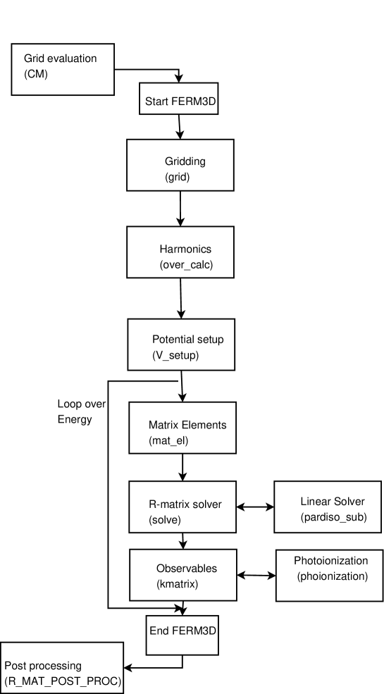
Figure 1: Code diagram. Each box shows the main function of a program/module, with the program names in capital letters, and in lowercase the module/subroutine names enclosed in parentheses.

The FERM3D package is made up of three codes: (1) the general scattering code (FERM3D.x), (2) an automatic grid utility (CM.x), and (3) a post-processing module (R_mat_post_proc.x) to extract differential cross sections and wavefunction maps [13]. The instructions for the compilation are inside the package. For each run, a set of four files from ab initio codes are required: electrostatic potential, electron density, norm and Laplacian. A script for Gaussian to calculate these files is also included in the distribution. From the quantum chemistry codes are also required: the spherical and nonspherical polarisabilities, the ionisation potential of the target and, for post-processing, the dipole moment magnitude and its components along the Cartesian axes. In the case of an ionic target, a photoionisation calculation can be performed, requiring the initial orbitals on a grid in the same format as for the potentials, and the ionisation potentials of these orbitals. Then the file input_control.dat should be set up (see Section IX). Afterwards, CM.x should be run to get the grid file. At this point the scattering calculation can be performed. When the calculation is completed, the post-processing code can be run to get supplementary information on the system as specified in Section VI. As shown in Fig. 1, the main code has the following structure : grid calculation (performed in subroutine grid), numerical harmonics calculations (over_calc), potential setup (V_setup), matrix elements setup (mat_el). Next comes the linear system solution (lin_rmatsparse) and the calculation of cross sections (kmatrix). Finally, an optional photoionisation calculation (photoionisation) can be run. Some subroutines in the code have been taken from Numerical Recipes [35], others from the Computer Physics Communications library [36], and others from other sources. All sources are cited in detail in the code.

As already stated, a number of third party libraries are used in this code, some necessary, some optional. Blas/Lapack are needed throughout the code, and a direct sparse solver (SuperLU in routine ”dSLUsolve” or Pardiso in ”pardiso_sub”) is also needed, since the large matrices generated by this code cannot be handled using a dense solver, even for a small target molecule. Optional libraries are Arpack[37], used to calculate surface harmonics in routine ”over_calc” together with the sparse solvers (otherwise a dense solver is used, for small/medium targets there is no difference in performance) and Cernlib, used in the post-processing utility. This is shown in Tab. 1.

Libraries	Intel	Alpha	SuperLU
Fortran Compiler	ifc (Intel, v9.0.027)	f90 (HP, v.V5.4-1283)	f90
C Compiler			gcc(v.3.0.1)
General	Lapack(v.3.0)	Lapack	Lapack
Eigenvalue	Arpack(v.96)
Linear system	Pardiso(v.3.0)	Pardiso	SuperLU(v.2.0)
Post processing	Cernlib(v.2004)

Table 1: Libraries needed to link the three different sample versions of the code given with the package, for alpha and Intel platforms. The Intel version shown here also uses the optional Arpack and Cernlib libraries, which can be avoided. in parentheses is indicated the version of the libraries used here. Essentially all possible library combinations can be utilized, i.e. using SuperLU on Intel platforms and so on. To interface the code with SuperLU 3.0 the bridge routine dSLUsolve.c will have to be modified.

IX Input description

Here we summarize the input file structure for the codes. In the input files reproduced below, the first entry (or two in the case of two variables per line) for each line corresponds to a sample value for the variable, e.g. for the CO₂ examples we show here. On the right side, there are comments including the name of the variable in the code and some brief descriptions. The input to CM.x is the file CM.dat, which specifies the maximum spacing per dimension. The output file is fort.16 which should be copied into input_grid.dat. The structure of CM.dat is:

12.d0         ! R0 = R-matrix box size
0.125         ! Delta_theta_max = Delta theta max
0.125         ! Delta_phi_max = Delta phi max
0.125         ! Delta_r_max = Delta R max (internal)
.5d0          ! Delta_external_radius = R max (external)

where the first entry defines the R-matrix box size R0. The box should contain the molecule and be completely contained in the cubical grid files output from ab initio programs for the potentials. A value of R0 from 10 to 14 Bohrs is usually appropriate for most of the molecules we have worked with. The other inputs define a maximum size of the finite element sectors in $\theta$, $\phi$ (both in units of $\pi$), and $r$. In the case of the radial dimension, two areas are defined, internal ($r<$r_cutoff which is defined below) and external. All the variables in this file are real and double precision. Also this code takes as input some quantities from input_control.dat, which is described below.

The grid spacing is fundamental for the convergence of the calculation. In simple molecules like CO₂, our gridding utility can easily do a good job of ensuring convergence while guaranteeing a low memory usage. For larger molecules some manual adjusting of the grid, especially around the nuclei, is often required. It is necessary for the convergence of the integrals to have a grid point at the position of each nucleus. For a correct representation of the wavefunction, it is also advisable to have grid points near the K-shell radius of the nuclei. CM.x constructs grids taking these factors into account, but verification of the convergence of the results (for example increasing the number of points in some of the dimensions by 50% or so) is critical for validation of the results, in other words, especially for inexperienced users that do not yet know what grid spacings should be used in each dimension, the first run on a molecule can give unconverged results that will not be very meaningful. Also, we have verified time and again that the angular grid spacings are more critical than the radial ones, since for atoms far off center of the grid, the $\theta$ and $\phi$ angles are usually described more poorly. Usually a spacing of $0.0625\pi$ in the angular variables outside the nuclei K-shell is fine enough for most molecules. In the examples we give here $0.125\pi$ is enough to get satisfying convergence since CO₂ is a compact target, while in benzene the atoms far from the grid center are hydrogens.

The main code has input_grid.dat and input_control.dat as input files. Data files named pot.dat, dens.dat, grad.dat, and nabla.dat must be created for the potential, density, norm of the gradient and Laplacian respectively, using output from ab initio codes. The input for the post-processing module is included in input_control.dat. This file has the following structure for the CO₂ example discussed in this paper:

950             ! output_file = File number for elastic cross section
scatter   nowf  ! calculation_type, option_wf
slater    8     ! type of exchange (obsolete),max_l
ion       1.0d0 ! molecule,  charge = residual molecular charge
8.95d0          ! polar = spherical polarisability
4.595d0         ! polar2 = nonspherical polarisability
3.7d0           ! r_cutoff = cutoff radius for DFT polarisation
0.90d0          ! Energy_last_bound = Ionisation potential
0.d0            ! shift = shift on z axis
1.2d0           ! Emax = Energy max
0.0d0           ! Emin = Energy min
12              ! nEmax = number of energy points
.0d0            ! shifty = shift on y axis
.FALSE.         ! rotation = swapping of y,z axes
.TRUE.          ! option_DFT = DFT correlation
0.d0            ! shiftx = shift on x axis
no              ! restore (obsolete)
no        0.d0   0.d0  0.d0  0.d0  ! option_DCS, dipole(5)


!!!! PHOTOIONIZATION INPUT !!!!!!!!!!
3   length      ! num_initial_states = Number of initial orbitals, gauge
pi_u_1.dat      ! orbital_name1 = Initial orbital file for photoionisation
0.71            ! Ioniz_potential = Ionisation potential for the initial state
sigma_g_4.dat
0.71
homo.dat
0.54

Now we will describe various variables, which have not been explained above. We indicate the name of the variable, with its type in parentheses. In our description, I stands for integer, R for double precision real, S for strings, all of which are of length 10 except orbital_name1 which can be of length 16, Then we explain the variable’s meaning and, for string variables, the values they can assume:
General part:
output_file = (I) redirects the output elastic cross section to file fort.output_file.
calculation_type = (S) defines the kind of calculation wanted, e.g. scattering (value = scatter) or bound-state problem (value = bound) to get the bound states of the potential.
option_wf = (S) sets the print switch for the scattering wavefunction, either to print (value = wf) or not (value = nowf) the eigenvector associated with the largest eigenvalue of the time-delay matrix of Eq. 12.
max_l = (I) maximum continuum angular momentum included (highest partial wave included in the calculation).
molecule = (S) defines the molecule type, which can be a neutral (value = neutral) or positive ion (value = ion).
polar, polar_2 = (R) represent one half of $\alpha_{0}$ and $\alpha_{2}$ in Eq. 5 respectively.
r_cutoff = (R) ensures the uniqueness of the crossing point between the DFT and asymptotic polarisation potentials. This variable should be set to a value roughly two atomic units larger than the radius of the atom farthest from the grid center.
Energy_last_bound = (R) defines the ionisation potential of the target, and enters the calculation from Eq. 2.
shift, shifty, shiftx = (R) coordinates translation for the whole molecule on the three Cartesian axes (largely unnecessary, but can be used to try to minimise the memory requirements).
option_DFT = (S) offers a choice between DFT correlation (value = DFT, strongly recommended) and semiempirical (value different from DFT), as in Ref. [12].
option_DCS = (S) creates a switch in post-processing for the differential cross section, to print it (value = yes) or not (value = no).
dipole = (R) constituted by an array of four numbers, the first of which is the absolute value of the dipole, the other three its x,y,z components. After these variables there are three blank lines for eventual future development.
Photoionisation part (only required for ions):
num_initial_states = (I) specifies the total number of initial orbitals to photoionise from.
option_gauge = (S) specifies which gauge to use to calculate the dipole matrix element (can assume value=length, which is the default, or value=velocity). For each initial orbital (1 to num_initial_states) the filename orbital_name1(S), which can assume any value, and the ionisation potential, Ioniz_potential(R), of the orbital are specified.

The code checks the correctness of the input options, and in case they are erroneous (for example a negative polarisability), it flags an error and exits. It is worth noticing that error checking is done on the grids as well, however this is not completely foolproof, as some subtle errors might not be caught by the checking done here. In these cases though, we have verified that the linear solver will exit before completion, flagging an error.

For the examples included in the package, the input files are in the directory ”examples” for each of the given tests. The inputs and outputs are included for each example in separate subdirectories, and the file structure is explained in a README file.

X Output description

Sample calculations for the photoionisation of CO${}_{2}^{+}$, total elastic and differential elastic cross sections of CO₂ and elastic scattering off of benzene are illustrated in Figs. 2,3,5,4 respectively. The program can output total elastic cross sections (file number set in input_control.dat, as specified in Sec.IX), phase shifts (phase_shifts.out), S-matrices (fort.536), total photoionisation cross sections from Eq. 10 (fort.951 and following, one for each initial state orbital), the dipole matrix elements $d^{(-)}_{\beta}$ in Eq. 10 (momenta.out). Through the post-processing modules, differential cross sections (fort.100 and following, one for each energy point calculated), eigenvectors of the time-delay matrix (fort.13001), elastic cross sections and S-matrices with a dipole potential outside the R-matrix box (fort.1280 and fort.538, respectively) can be output as well. Many of these quantities are also written to standard output. The matrices are all written by columns, the wavefunction file contains the x, y and z coordinates of the point and the wavefunction value, in this order. The other files all have the energy in the first column and the quantity of interest in the second.

For the examples given in the package, the output files for total elastic and photoionisation cross sections (together with the input scripts) are listed in the directory ”examples” of the tar file. The figures included in this article were generated using the examples given.

In general, the approximations made in the model are such that the resonant structures will appear shifted too high with respect to experimental values, in many cases we have seen that this shift is roughly of the order of a couple of eV, as for the DNA bases [13] and THF [38] and also for smaller molecules like carbon dioxide, benzene, as shown in Figs. 3 and 4 and SF₆,[39]. The fact that our resonances are shifted too high in energy can in turn cause the width to be larger than the experimental one. We have verified in the past for many systems [13, 39] that our calculated widths are usually close to their correct values.

The model potential we use here has been used extensively in the literature, in particular a comparison is possible with data from Gianturco and co-workers, we will cite the values of the resonances we found for the benzene molecule, and compare to the ones listed in Table II of Ref. [40]. In our calculations the resonances are at 3.4eV, 9.2 eV, 13.2, compared to values of 4.66, 9.02, 12.25, so the values are quite similar. Also the widths are quite similar. It is not possible to compare directly the cross sections because this data is not available from Ref. [40], however we will compare with their results using correct (nonlocal) exchange, which shifts all their resonances down by a few eV, in Fig. 4. It is important to notice how in this case the higher resonances have roughly the same widths between the model potential and exact exchange calculations, while the lowest one becomes much narrower and it is shifted down by 3eV with respect to the others. In Ref. [12] we have also compared to the results of Morrison and Collins [14] for CO₂, using the same adjustable polarisation potential used in that work. We have shown how those results are very similar to our calculations in that case. In Fig. 3 we also compare our results for CO₂ with those of Refs. [3] (exact static exchange, SE, and exchange plus polarisation, SEP) and [14] (local exchange plus semiempirical polarisation). For larger molecules, the only comparison possible is with the results of Gianturco $et$ $al.$ on uracil [11], which we have given in detail in Ref. [13] and will not be repeated here.

XI Conclusions

We have presented the FERM3D package, a general code for performing electron molecule scattering and photoionisation calculations. The code is very versatile and can be used to extract, with predictive value, elastic cross sections, resonance structures, and photoionisation cross sections. No use is made of symmetry, whereby the code performs well for molecules with low symmetry, such as the DNA bases, which are difficult to explore with more sophisticated approaches.

Figure 2: CO₂ photoionisation cross section for the three highest valence orbitals ($\pi_{u}$, $\pi_{g}$, $\sigma_{g}$), which generate the doublet final states in the figure. Comparison with the results of Lucchese et al. [41] is very good. In our calculation the $\sigma_{u}$ resonance is shifted roughly 1 eV higher with respect to Ref. [41].

Figure 3: CO₂ elastic cross section at low energies. The prominent structure is the well-known $\pi_{u}$ resonance which, in experiment, has been found at 3.8 eV. Often the resonances we calculate with our approach are roughly 2-2.5 eV higher if compared to experimental values, see e.g. Fig. 4 in Ref. [12]. Our results are compared with those of Rescigno $et$ $al.$ [3] (exact static exchange and exchange plus polarisation) and Morrison and Collins [14] (model exchange plus semiempirical polarisation). The resonance width is larger than the SEP results of Rescigno $et$ $al.$ but comparable to the other calculations.

Figure 4: Benzene elastic cross section at low energies. Comparison with the exact exchange plus model polarization results of Gianturco $et$ $al.$ [40]. The comparison of the resonance positions with the model exchange results of Ref. [40] are given in the text.

Figure 5: CO₂ differential cross section at four selected low electron impact energies. The results can be compared with those of Ref. [3, 29, 31, 32].

References

- [1] B. Boudaiffa, P. Cloutier, D. Hunting, M. A. Huels, L. Sanche, Science 287 (2000) 1658.
- [2] B. J. McCall, T. Oka, Science 287 (2000) 1941.
- [3] T. N. Rescigno, D. A. Byrum, W. A. Isaacs, C. W. McCurdy, Phys. Rev. A 60 (1999) 2186.
- [4] M. Allan, T. Skalicky, J. Phys. B 36 (2003) 3397.
- [5] A. Scheer, K. Aflatooni, G. A. Gallup, P. D. Burrow, Phys. Rev. Lett. 92 (2004) 068102.
- [6] R. R. Lucchese, F. A. Gianturco, N. Sanna, Chem. Phys. Lett. 305 (1999) 413.
- [7] F. A. Gianturco, R. R. Lucchese, J. Chem. Phys. 114 (2001) 3429.
- [8] D. Bouchiha, J. D. Gorfinkiel, L. G. Caron, L. Sanche, J. Phys. B 39 (2006) 975.
- [9] C. N. Trevisan, A. E. Orel unpublished.
- [10] S. d’A. Sanchez, C. Winstead, V. McKoy, in: Book of abstracts 24th International Conference on Photonic Electronic and Atomic Collisions, 2005.
- [11] F. A. Gianturco, R. R. Lucchese, J. Chem. Phys. 120 (2004) 7446.
- [12] S. Tonzani, C. H. Greene, J. Chem. Phys. 122 (2005) 014111.
- [13] S. Tonzani, C. H. Greene, J. Chem. Phys. 124 (2006) 054312.
- [14] M. Morrison, L. A. Collins, Phys. Rev. A 17 (1978) 918.
- [15] S. Hara, J. Phys. Soc. Jpn. 27 (1969) 1009.
- [16] Bioengineering Institute, The University of Auckland, New Zealand, Fem/bem notes, http://www.bioeng.auckland.ac.nz/cmiss/fembemnotes/fembemnotes.pdf (February 1997).
- [17] K. J. Bathe, Finite Element Procedures, Prentice-Hall, Englewood Cliffs, N. J., 1996.
- [18] C. H. Greene, M. Aymar, E. Luc-Koenig, Rev. Mod. Phys. 68 (1996) 1015.
- [19] J. Tennyson, J. Phys. B 37 (2004) 1061.
- [20] N. F. Lane, Rev. Mod. Phys. 52 (1980) 29.
- [21] F. A. Gianturco, J. A. Rodriguez-Ruiz, Phys. Rev. A 47 (1993) 1075.
- [22] R. Colle, A. Salvetti, J. Chem. Phys. 19 (1983) 1404.
- [23] C. Lee, W. Yang, R. G. Parr, Phys. Rev. B 37 (1988) 785.
- [24] J. A. Pople, et al., GAUSSIAN98, Pittsburgh, http://www.gaussian.com (1998).
- [25] H. J. Werner, P. J. Knowles, R. Lindh, M. Schutz, et al., MOLPRO, a package of ab initio programs, Birmingham, UK, http://www.molpro.net (2003).
- [26] A. A. Granovsky, PC-GAMESS, http://classic.chem.msu.su/gran/gamess/index.html.
- [27] S. Tonzani, Ferm3d website, http://fermion.colorado.edu/~tonzani/Software/rmatrix/Software.html (2006).
- [28] D. Dill, J. L. Dehmer, J. Chem. Phys. 61 (1974) 692.
- [29] F. A. Gianturco, T. Stoecklin, J. Phys. B 29 (1996) 3933.
- [30] CERN, Cernlib, http://wwwasd.web.cern.ch/wwwasd/cernlib/.
- [31] M. A. Morrison, N. F. Lane, L. A. Collins, Phys. Rev. A 15 (1977) 2186.
- [32] J. C. Gibson, M. A. Green, K. W. Trantham, S. J. Buckman, P. J. O. Teubner, M. J. Brunger, J. Phys. B 32 (1999) 213.
- [33] S. Li and J. Demmel and J. Gilbert, Superlu, http://crd.lbl.gov/ xiaoye/SuperLU/.
- [34] Scientific Computing Group, University of Basel, Pardiso, http://www.computational.unibas.ch/cs/scicomp/software/pardiso/.
- [35] G. H. Press, B. P. Flannery, S. A. Teukolsky, W. T. Vetterling, Numerical Recipes in Fortran, Cambridge University Press, Cambridge, 1995.
- [36] Computer Physics Communications library, http://www.cpc.qub.ac.uk.
- [37] R. Lehoucq and K. Maschhoff and D. Sorensen and C. Yang, Arpack, http://www.caam.rice.edu/software/ARPACK/ (1996).
- [38] S. Tonzani, C. H. Greene, J. Chem. Phys. submitted.
- [39] S. Tonzani, C. H. Greene unpublished.
- [40] F. A. Gianturco, R. R. Lucchese, J. Chem. Phys. 108 (1998) 6144.
- [41] R. R. Lucchese, V. McKoy, Phys. Rev. A 26 (1982) 1406.