Power-law behavior and condensation phenomena in disordered urn models

Abstract

We investigate equilibrium statistical properties of urn models with disorder. Two urn models are proposed; one belongs to the Ehrenfest class, and the other corresponds to the Monkey class. These models are introduced from the view point of the power-law behavior and randomness; it is clarified that quenched random parameters play an important role in generating power-law behavior. We evaluate the occupation probability $P(k)$ with which an urn has $k$ balls by using the concept of statistical physics of disordered systems. In the disordered urn model belonging to the Monkey class, we find that above critical density $\rho_{\mathrm{c}}$ for a given temperature, condensation phenomenon occurs and the occupation probability changes its scaling behavior from an exponential-law to a heavy tailed power-law in large $k$ regime. We also discuss an interpretation of our results for explaining of macro-economy, in particular, emergence of wealth differentials.

1 Introduction

A lot of techniques and concepts of statistical mechanics of disordered spin systems, in particular, the replica method originally used to analyze the thermodynamics of spin glass model by Sherrington and Kirkpatrick [1], have been applied to various research fields beyond conventional physics, i.e. information processing [2], game theory [3] and so on. The exactly solvable mathematical model, which describes these problems, is categorized as mean-field class [4].

On the other hand, as another exactly tractable model, in 1907, Paul and Tatiana Ehrenfest published a paper corroborating Boltzmann’s view of thermodynamics [5]. Their urn model has been defined by Kac [6] as an exactly solvable example in statistical physics. While it has also been criticized as a marvelous exercise too far removed from reality, their urn model has been applied to modern problems such as complex networks [7, 8] or econophysics [9, 10], etc. For instance, based on extensive simulations of the Lennard-Jones fluid requiring in part a parallel computer in Juelich, an Italian-German team has shown that the prediction of the Ehrenfest urn effectively describes the behavior of the gas phase [11]. Moreover, it has been revealed that the mathematical structure of equilibrium state of the urn model [12] is similar to the zero-range process, which has been widely investigated in research fields of non-equilibrium statistical physics [13].

Recently, in the research field of complex networks [7, 8], Ohkubo et al. [14] proposed a network model based on ‘Ehrenfest class urn model’ to explain how the complex network gets scale-free-like properties, where ‘Ehrenfest class’ means that each urn has distinguishable balls. In the model, each urn corresponds to a node in graph (network) and the number of distinguishable balls, $k$, in each urn is regarded as degree of nodes. For this model system, they succeeded in deriving the scale-free-like properties $\sim k^{-2}(\log k)^{-2}$ in the probability of the degree of nodes by the usage of the replica symmetric theory [15]. In addition, the similarity between the disordered urn model and the random field Ising model [16], and the condensation phenomena in the disordered urn model have been investigated [17].

We here note that there are a lot of works in which the power-law behavior and the condensation phenomena in urn models have been studied [12, 18]. For example, in the zeta urn model [12], the power-law behavior in the probability of the number of balls, i.e., the occupation distribution, stems from a power-law form of the Boltzmann weight. However, when we attempt to describe various problems in the real world, we should take into account the disorder and treat the urns as a heterogeneous system. Mainly, the previous models which cause power-law behavior in the occupation distribution do not contain any disorder, and hence it would be important to investigate ‘disordered’ urn models which cause the power-law distribution.

In this paper, we propose two disordered urn models in which quenched randomness is important for generating the power-law behavior. One of them belongs to the Ehrenfest class, and the other corresponds to the Monkey class, in which each urn has indistinguishable balls. In particular, for the Monkey class urn model, we investigate a real-space condensation phenomenon in which macroscopic number of balls are condensed into only one urn. The occupation probability $P(k)$ with which an urn has $k$ balls is calculated analytically, and furthermore, the critical density $\rho_{\rm c}$ for a given temperature is evaluated. As the result, it is shown that the occupation distribution function $P(k)$ changes its scaling behavior from the exponential $k^{-(\alpha+1)}\,{\rm e}^{-k}$-law to the $k^{-(\alpha+2)}$ power-law in large $k$ regime.

This paper is organized as follows. In the next section 2, we introduce the general formalism for the urn model with an arbitrary energy function. Although there are several analytical treatments for disordered urn models [15, 19], we give the formalism for the disordered urn model with an arbitrary energy function with a different point of view, and additionally, the analytical treatment makes this paper self-contained. This analytical treatment contains both Ehrenfest and Monkey classes as its special cases. We explain the relation between the saddle point, that determines the thermodynamic properties of the system, and the chemical potential. With the assistance of this general formalism, we provide an analysis for a special choice of the energy function, which is an example of the Ehrenfest class in section 3. We discuss the condition on which the power-law appears in the tail of the occupation probability for the model. In section 4, we show that the condensation occurs for the special case of the Monkey class with disorder, and a heavy tailed power-law emerges in the occupation probability. In section 5, we provide a possible link between our results and macro economy, in particular, wealth differentials. Last section is a summary.

2 General formalism for urn models with disorder

Let us prepare $N$ urns and $M$ balls ($M\equiv\rho N$) and consider the situation in which the $N$ urns share the $M$ balls. Then, we start our argument from the Ehrenfest class urn model [12] in which each ball in urns is distinguishable. For the mathematical model categorized in the Ehrenfest class, the Boltzmann weight $p(n_{i})$ that $i$-th urn possesses $n_{i}$ balls is given by

$$p(n_{i}) = \frac{{\exp}\left[-\beta E(\epsilon_{i},n_{i})\right]}{n_{i}!},$$ (1)

where $E(\epsilon_{i},n_{i})$ is an energy function, $\epsilon_{i}$ a disorder parameter for urn $i$, and $\beta$ the inverse temperature of the system. The factorial $n!$ stems from the property of the Ehrenfest class [12]. The only point of our analysis which is different from [12] is quenched disorder $\epsilon_{i}$ appearing in the energy function. For the Ehrenfest class, the probability that an urn specified by the disorder parameter $\epsilon_{1}$ possesses $k$ balls is given by

$$f_{k}^{(\epsilon_{1})}(\{\epsilon_{i/1}\})=\frac{1}{Z_{1}}\,\sum_{n_{1}=0}^{\infty}\cdots\sum_{n_{N}=0}^{\infty}\delta(n_{1},k)\,p(n_{1})\cdots p(n_{N})\,\delta\left(\sum_{i=1}^{N}n_{i},M\right)$$

$$\mbox{}=\frac{e^{-\beta E(\epsilon_{1},k)}}{k!}\frac{1}{Z_{1}}\prod_{i=2}^{N}\left[\sum_{n_{i}=0}^{\infty}\left(\frac{{\rm e}^{-\beta E(\epsilon_{i},n_{i})}}{n_{i}!}\right)\right]\oint\frac{dz}{2\pi i}{\exp}\left[\left(k+\sum_{i=2}^{N}n_{i}-M-1\right)\log z\right]$$

$$\mbox{}=\frac{e^{-\beta E(\epsilon_{1},k)}}{k!}\left(\frac{Z_{2}}{Z_{1}}\right),$$ (2)

where $\{\epsilon_{i/1}\}\equiv\{\epsilon_{2},\cdots,\epsilon_{N}\}$ and we defined $Z_{2}$ as

$$Z_{2}=\prod_{i=2}^{N}\left[\sum_{n_{i}=0}^{\infty}\left(\frac{{\rm e}^{-\beta E(\epsilon_{i},n_{i})}}{n_{i}!}\right)\right]\oint\frac{dz}{2\pi i}{\exp}\left[\left(k+\sum_{i=2}^{N}n_{i}-M-1\right)\log z\right],$$ (3)

and used the Fourier transform of the Kronecker-delta:

$$\delta(A,B) = \oint\frac{dz}{2\pi i}\,z^{A-B-1}$$ (4)

to introduce the conservation of the total balls : $n_{1}+\cdots+n_{N}=M\equiv\rho N$ into the system. In order to calculate $P(k)$, we take the configuration average of $f_{k}^{(\epsilon_{1})}(\{\epsilon_{i/1}\})$. While one can calculate the configuration average by means of the replica method [15], it has been revealed that the mathematical structure of the disordered urn model is related to that of a random field Ising model [16]. Hence, we here use the law of large numbers and simplify the calculation. To calculate the average of the quantity $\exp[\log f_{k}^{(\epsilon_{1})}(\{\epsilon_{i/1}\})]$ over the configuration $\{\epsilon_{1},\cdots,\epsilon_{N}\}$, we consider the Tayler-expansion:

$$\langle\exp[\log f_{k}^{(\epsilon_{1})}(\{\epsilon_{i/1}\})]\rangle_{\{1,2,\cdots,N\}} = 1+\langle\log f_{k}^{(\epsilon_{1})}(\{\epsilon_{i/1}\})\rangle_{\{1,2,\cdots,N\}}$$ (5)

$$+ \frac{1}{2}\langle(\log f_{k}^{(\epsilon_{1})}(\{\epsilon_{i/1}\}))^{2}\rangle_{\{1,2,\cdots,N\}}+\cdots$$

where $\langle\cdots\rangle_{\{1,2,\cdots,N\}}$ means the configuration average over $\{\epsilon_{1},\cdots,\epsilon_{N}\}$. Here we assume that the observable $\log f_{k}^{(\epsilon_{1})}(\{\epsilon_{i/1}\})$ for a given realization of configuration $\{\epsilon_{1},\cdots,\epsilon_{N}\}$ is almost identical to the average $\langle\log f_{k}^{(\epsilon_{1})}(\{\epsilon_{i/1}\})\rangle_{\{1,2,\cdots,N\}}$. In other words, the deviation is vanishingly small as $\langle(\log f_{k}^{(\epsilon_{1})}(\{\epsilon_{i/1}\}))^{2}\rangle_{\{1,2,\cdots,N\}}-\langle\log f_{k}^{(\epsilon_{1})}(\{\epsilon_{i/1}\})\rangle_{\{1,2,\cdots,N\}}^{2}\simeq 0$ in the thermodynamics limit. By using the assumption, we rewrite (5) as follows.

$$\langle\exp[\log f_{k}^{(\epsilon_{1})}(\{\epsilon_{i/1}\})]\rangle_{\{1,2,\cdots,N\}} \simeq 1+\langle\log f_{k}^{(\epsilon_{1})}(\{\epsilon_{i/1}\})\rangle_{\{1,2,\cdots,N\}}+\frac{1}{2}\langle\log f_{k}^{(\epsilon_{1})}(\{\epsilon_{i/1}\})\rangle_{\{1,2,\cdots,N\}}^{2}$$ (6)

$$+ \cdots=\exp[\langle\log f_{k}^{(\epsilon_{1})}(\{\epsilon_{i/1}\})\rangle_{\{1,2,\cdots,N\}}]$$

This replacement of the configuration average reads

$$\langle f_{k}^{(\epsilon_{1})}(\{\epsilon_{i/1}\})\rangle_{\{1,2,\cdots,N\}}=\left\langle\exp\left(\log f_{k}^{(\epsilon_{1})}(\{\epsilon_{i/1}\})\right)\right\rangle_{\{1,2,\cdots,N\}}\simeq\exp\left(\langle\log f_{k}^{(\epsilon_{1})}(\{\epsilon_{i/1}\})\rangle_{\{1,2,\cdots,N\}}\right)$$

$$=\exp\left(\left\langle\log[e^{-\beta E(\epsilon_{1},k)}/k!]+\langle\log Z_{2}\rangle_{\{2,3,\cdots,N\}}-\langle\log Z_{1}\rangle_{\{2,3,\cdots,N\}}\right\rangle_{\{1\}}\right).$$ (7)

In the thermodynamic limit $N\to\infty$, $\langle\log Z_{2}\rangle_{\{2,3,\cdots,N\}}$ is evaluated as

$$\langle\log Z_{2}\rangle_{\{2,3,\cdots,N\}}=\left\langle\log\left(\oint\frac{dz}{2\pi i}z^{k-M-1}\prod_{i=2}^{N}\left\{\sum_{n_{i}=0}^{\infty}\frac{{\rm e}^{-\beta E(\epsilon_{i},n_{i})}}{n_{i}!}z^{n}\right\}\right)\right\rangle_{\{2,3,\cdots,N\}}$$

$$=\left\langle\log\left(\oint\frac{dz}{2\pi i}\exp\left[(k-\rho N-1)\log z+\sum_{i=2}^{N}\left\{\log\sum_{n_{i}=0}^{\infty}\frac{{\rm e}^{-\beta E(\epsilon_{i},n_{i})}}{n_{i}!}z^{n}\right\}\right]\right)\right\rangle_{\{2,3,\cdots,N\}}$$

$$\simeq\log\left(\oint\frac{dz}{2\pi i}\exp\left[(k-\rho N-1)\log z+(N-1)\left\langle\log\sum_{n=0}^{\infty}\frac{{\rm e}^{-\beta E(\epsilon,n)}}{n!}z^{n}\right\rangle\right]\right)$$

$$\simeq k\log z_{s1}-(\rho N+1)\log z_{s1}+(N-1){\biggr{\langle}}\log\sum_{n=0}^{\infty}\frac{{\rm e}^{-\beta E(\epsilon,n)}}{n!}z_{s1}^{n}{\biggr{\rangle}},$$ (8)

where we used the law of large numbers, and in the final line the saddle point method was used. $\langle\cdots\rangle$ means the average over only $\epsilon$, namely, $\langle\cdots\rangle\equiv\int(\cdots)D(\epsilon)d\epsilon$. In the next two sections, we consider specific choices of $D(\epsilon)$ to evaluate the occupation probability distribution concretely. Using the same way as the $Z_{2}$, $Z_{1}$, which is obtained by the normalization condition of $f_{k}^{(\epsilon_{1})}$, namely, $\sum_{k=0}^{\infty}f_{k}^{(\epsilon_{1})}=1$ with equation (2), is rewritten as

$$\langle\log Z_{1}\rangle_{\{2,3,\cdots,N\}}$$

$$=\log\sum_{k=0}^{\infty}\frac{{\rm e}^{-\beta E(\epsilon_{1},k)}}{k!}z_{s2}^{k}-(\rho N+1)\log z_{s2}+(N-1){\biggr{\langle}}\log\sum_{n=0}^{\infty}\frac{{\rm e}^{-\beta E(\epsilon,n)}}{n!}z_{s2}^{n}{\biggr{\rangle}}.$$ (9)

We easily find $z_{1s}=z_{2s}$ because the first terms for each saddle point equation (8) or (9) are vanishingly smaller than the other two terms in the limit of $N\to\infty$.

Thus, we obtain the saddle point equation with respect to $z_{s}\equiv z_{s1}=z_{s2}$ and the occupation probability $P(k)=\langle f_{k}^{(\epsilon)}\rangle$ that an arbitrary urn with the energy function $E$ at inverse temperature $\beta$ has $k$ balls are given by

$$\rho z_{s}^{-1} = {\biggr{\langle}}\frac{\sum_{n=0}^{\infty}n\frac{{\rm e}^{-\beta E(\epsilon,n)}}{(n-1)!}z_{s}^{n-1}}{\sum_{n=0}^{\infty}\frac{{\rm e}^{-\beta E(\epsilon,n)}}{n!}z_{s}^{n}}{\biggr{\rangle}}$$ (10)

and

$$P(k) = {\biggr{\langle}}\frac{\frac{{\rm e}^{-\beta E(\epsilon,k)}}{k!}z_{s}^{k}}{\sum_{n=0}^{\infty}\frac{{\rm e}^{-\beta E(\epsilon,n)}}{n!}z_{s}^{n}}{\biggr{\rangle}},$$ (11)

respectively. It should be noticed that the above saddle point equation for the Ehrenfest class urn model (10) is now rewritten in terms of chemical potential

$$\mu \equiv \beta^{-1}\log z_{s}$$ (12)

as

$$\rho = {\biggr{\langle}}\frac{\sum_{n=0}^{\infty}n\frac{{\rm e}^{-\beta[E(\epsilon,n)-n\mu]}}{n!}}{\sum_{n=0}^{\infty}\frac{{\rm e}^{-\beta[E(\epsilon,n)-n\mu]}}{n!}}{\biggr{\rangle}}.$$ (13)

Then, we define the probability $p_{n}$ that an arbitrary Ehrenfest class urn with energy $E$ has $n$ balls by

$$p_{n} = \frac{\phi_{E,\mu,\beta}(\epsilon,n)}{\sum_{n=0}^{\infty}\phi_{E,\mu,\beta}(\epsilon,n)},\,\,\,\,\,\phi_{E,\mu,\beta}(\epsilon,n)=\frac{{\rm e}^{-\beta[E(\epsilon,n)-n\mu]}}{n!}.$$ (14)

From this formula of the probability $p_{n}$ with the effective Boltzmann factor $\phi_{E,\mu,\beta}(\epsilon,n)$, the equation (13) means that the ratio $M/N$ corresponds to the average number of balls put in an arbitrary urn: $\rho=\sum_{n=0}^{\infty}n\phi_{E,\mu,\beta}(\epsilon,n)/\sum_{n=0}^{\infty}\phi_{E,\mu,\beta}(\epsilon,n)$, and its value is controlled by the chemical potential $\mu$ through the equation (13). Then, the chemical potential $\mu$ and the saddle point $z_{s}$ are related through the equation (12). Therefore, when we construct the system so as to have a density $\rho$, the corresponding saddle point $z_{s}$ is given by (13). As the result, the chemical potential $\mu$ that gives $\rho$ is determined by the relation (12).

Thus, our problem is now to solve the saddle point equation

$$\rho = {\biggr{\langle}}\frac{\sum_{n=0}^{\infty}n\,\phi_{E,\mu,\beta}(\epsilon,n)}{\sum_{n=0}^{\infty}\phi_{E,\mu,\beta}(\epsilon,n)}{\biggr{\rangle}},$$ (15)

and to calculate the following averaged occupation probability for the solution $z_{s}={\rm e}^{\beta\mu}$ of the equation (15):

$$P(k) = {\biggr{\langle}}\frac{\phi_{E,\mu,\beta}(k)}{\sum_{n=0}^{\infty}\phi_{E,\mu,\beta}(\epsilon,n)}{\biggr{\rangle}}.$$ (16)

Now it is time for us to stress that the Ehrenfest or Monkey class is recovered if we choose the effective Boltzmann factor $\phi_{E,\mu,\beta}(\epsilon,n)$ as follows [12].

$$\phi_{E,\mu,\beta}(\epsilon,n) = \left\{\begin{array}[]{ll}(n!)^{-1}\,{\exp}\left[-\beta(E(\epsilon,n)-n\mu)\right]&(\mbox{Ehrenfest class}),\\ {\exp}\left[-\beta(E(\epsilon,n)-n\mu)\right]&(\mbox{Monkey class}).\end{array}\right.$$ (19)

It should be noted that in our formalism, the distinction between two models only comes from the difference of the effective Boltzmann factor (19). We here also comment on the effect of the disorder to the dynamics of urn models. In the uniform case without disorder, all urns are equivalent, and we do not distinguish each urn in the Monkey class. On the other hand, in the disordered urn model, each urn $i$ has own label $\epsilon_{i}$, and hence they are distinguishable at least in principle. However, we assume that this heterogeneity of urns does not change the “Monkey” nature in the Monkey class; we cannot see the disorder parameter assigned to each urn from outside, and the dynamics (so called ‘box-to-box choice’) is not changed.

3 Ehrenfest class urn model with disorders

As an demonstration of the Ehrenfest urn model whose thermodynamic properties are specified by equations (10) and (11), we introduce a kind of disordered Ehrenfest urn models and consider the condition on which the power-law appears. To this end, we choose the energy function $E(\epsilon,n)$ as

$$E(\epsilon,n) = -\epsilon n,$$ (20)

where $\epsilon$ means an urn-dependent disorder of the system, and we here assume that $\epsilon$ takes a value in the range $[0,1]$ randomly, that is, $D(\epsilon)=\Theta(\epsilon)-\Theta(\epsilon-1)$ with the step function $\Theta(\cdots)$. Of course, we might choose the other distribution $D(\epsilon)$, however, the main issue of this section is to examine whether the power-law appears in the occupation probability distribution when we introduce the disorder, and for this purpose, the simplest choice is enough. The tendency of this energy function to force each urn of the system to gather balls as much as possible results in the fact that the rich get richer as its collective behavior. We should mention that in [19], the co-called Backgammon model [20] described by the cost function $E(\epsilon_{i},n_{i})=-\epsilon_{i}\delta_{n_{i},0}$ for each urn was studied. In the model, the cost decreases if and only if each urn is empty. In this sense, the model we deal with in this section is regarded as an opposite situation of our model. Therefore, it is interesting to investigate whether there exists any significant difference or the similarity between two models from the view point of the occupation probability distribution. The extensive studies concerning this issue will be our future studies.

For this choice of the energy function (20), the saddle point equation (10) leads to

$$z_{s} = \frac{\beta\rho}{{\rm e}^{\beta}-1}.$$ (21)

From equation (11), the occupation probability for the choice (20), $P(k)$, is given by

$$P(k) = \frac{z_{s}^{k}}{k!}\int_{0}^{1}d\epsilon\,{\exp}\left(\beta\epsilon k-z_{s}{\rm e}^{\beta\epsilon}\right).$$ (22)

In following, we evaluate the above occupation probability. We first show the phase diagram that indicates the area of the power-law behavior.

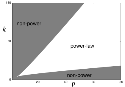
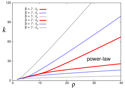
Figure 1: The $\rho$-$k$ phase diagrams concerning the heavy tailedness of the occupation probability. In the phase diagram for $\beta=3$ (left panel), the occupation probability follows non-power, exponential-law. The power-law regime exists for $\rho\geq\rho_{\rm b}=2.697423$. In the right panel, we plot the phase boundaries $k_{d},k_{u}$ as a function of density $\rho$ for several values of inverse temperature, namely, $\beta=2,3$ and $5$.

In Figure 1 (left), we show the phase diagram for the case of $\beta=3$. The shaded area in this figure means non-power, exponential-law region. From this figure, we find that while the upper bound (the cut-off) $k_{\rm u}$ and the lower bound $k_{\rm d}$ increase as the density $\rho$ increases, the cut-off $k_{\rm u}$ increases much more quickly than the lower bound $k_{\rm d}$. As the result, the heavy tailed power-law $k^{-1}$-region is broadened by increase of the density $\rho$. In the right panel of Figure 1, we display the inverse temperature dependence of the area of the power-law. As temperature increases, the area of the power-law shrinks to zero. Then, we have a Poisson-law in whole region of the phase diagram in the high-temperature limit of $\beta=0$.

We explain the detail of the evaluations as follows. We first consider the high-temperature limit $\beta=0$. For this case, the saddle point (21) leads to $z_{s}=\rho$ and we obtain

$$P(k) = \frac{\rho^{k}}{k!}\,{\exp}\left(-\rho\right),$$ (23)

which is nothing but a Poisson distribution.

For finite temperature $\beta>0$, the occupation probability $P(k)$ is rewritten as

$$P(k) = \frac{1}{\beta k!}\left[\Gamma_{k}\left(\frac{\beta\rho}{{\rm e}^{\beta}-1},\infty\right)-\Gamma_{k}\left(\frac{\beta\rho\,{\rm e}^{\beta}}{{\rm e}^{\beta}-1},\infty\right)\right],$$ (24)

where we defined the incomplete Gamma function by $\Gamma_{k}(a,b)=\int_{a}^{b}t^{k-1}{\rm e}^{-t}dt$. In Figure 2, we plot the occupation probability $P(k)$ for several values of $\rho$ for $\beta=3$, $z_{s}=0.5,1,2$ and $3$, namely, $\rho=3.180923,6.361846,12.723691$ and $19.085537$.

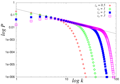
Figure 2: The Log-Log plot of occupation probability $P(k)$ as a function of $k$ for several values of $z_{s}$, namely, $z_{s}=0.5,1,2$ and $z_{s}=3$, namely, $\rho=3.180923,6.361846,12.723691$ and $19.085537$. We set the inverse temperature $\beta=3.0$. The right panel shows the behavior of $\Phi(k)$.

From this figure, we find that $P(k)$ obeys a power-law $\sim k^{-1}$ in the intermediate regime of $k$ and there exists a cut-off value from which the distribution decays exponentially. To see the existence of the cut-off value explicitly, we rewrite the distribution $P(k)$ as

$$P(k) = \frac{1}{\beta k}-\Phi(k),\,\,\,\,\,\Phi(k)\equiv\frac{1}{\beta k!}\left[\Gamma_{k}\left(0,\frac{\beta\rho}{{\rm e}^{\beta\rho}-1}\right)-\Gamma_{k}\left(\frac{\beta\rho\,{\rm e}^{\beta}}{{\rm e}^{\beta}-1},\infty\right)\right].$$ (25)

In Figure 2 (right), we plot the function $\Phi(k)$ for several values of $z_{s}$ at $\beta=3$. We easily find that in the range of $[k_{\rm d},k_{\rm u}]$ defined in terms of the function $\Phi(k)$ as $k_{\rm d}\equiv\min\{k|\Phi(k)=0\}$, $k_{\rm u}\equiv\max\{k|\Phi(k)=0\}$, the occupation probability $P(k)$ follows a power-law distribution $\sim k^{-1}$. Thus, we specified the region $(\rho,k)$ in which a power-law heavy tail appears in the occupation distribution as shown in Figure 1.

As shown in this section, for the Ehrenfest class disordered urn model, we could clarify the control parameters of the system for which the heavy tail power-law emerges in the occupation probability. In the next section, we consider a Monkey class urn model with disorders.

4 Bose-Einstein condensation and emergence of the heavy tail

In the previous section, we evaluated the asymptotic form of the occupation probability $P(k)$ for the urn model of the Ehrenfest class with energy function $E(\epsilon,n)=-\epsilon n$. Obviously, from the view point of the energy cost, it is a suitable strategy for each urn to gather balls as much as possible. In that sense, this case should be referred by the concept the rich get richer in the context of social networks. However, by using the general definition of the problem, we freely choose the energy function for both the Ehrenfest and Monkey classes.

In this section, for the Monkey class urn model whose thermodynamic properties are defined by equations (15), (16) and (19), we evaluate $P(k)$ for a specific choice of energy function $E(\epsilon,n)$. We choose the energy $E(\epsilon,n)$ as

$$E(\epsilon,n) = \epsilon n\,\,\,\,\,(\epsilon\geq 0).$$ (26)

We should notice that for this simple choice of the energy function, the urn labeled by $\epsilon\neq 0$ is hard to gather the balls. On the other hand, the urn with $\epsilon=0$ energy level easily gathers the balls. The urn model having this type of energy function does not agree with the concept the rich get richer. Nevertheless, we use the energy function (26) because as we shall see below, a kind of condensation with respect to the urns occurs for this choice of energy function, and as the result, the power-law in the tail of the occupation probability emerges.

For a given choice of $D(\epsilon)$ as the density of state, namely, degeneracy of the energy level of the urn, we rewrite the saddle point equation (15) as follows:

$$\rho = \int_{0}^{\infty}\frac{D(\epsilon)\,d\epsilon}{z_{s}^{-1}\,{\rm e}^{\beta\epsilon}-1}.$$ (27)

To proceed to the next stage of the calculation, we choose the density of state $D(\epsilon)$ explicitly as

$$D(\epsilon) = \varepsilon_{0}\sqrt{\epsilon},$$ (28)

where $\varepsilon_{0}$ is a constant. Although we chose the above form, more general setup of the argument by choosing $D(\epsilon)=\varepsilon_{0}\epsilon^{\alpha}$ is possible. We shall discuss the result for this kind of generalization later on. Then, the equation (27) is rewritten by

$$\rho = \int_{0}^{\infty}\frac{\varepsilon_{0}\sqrt{\epsilon}\,d\epsilon}{z_{s}^{-1}\,{\rm e}^{\beta\epsilon}-1}+\rho_{\epsilon=0},$$ (29)

where $\rho_{\epsilon=0}$ means the density of balls in the urn labeled by the zero-energy level $\epsilon=0$. We should notice that the second term appearing in the right hand side of equation (29), namely, $\rho_{\epsilon=0}$ vanishes in the thermodynamic limit $N\to\infty$ when a condensation does not occur. In other words, when the condensation arises, the second term, $\rho_{\epsilon=0}$, becomes from zero to a finite value; this means that an urn with $\epsilon=0$ becomes to have a macroscopic number of balls.

In following, we show the system undergoes a condensation and investigate the behavior of the system when the density $\rho$ increases beyond the critical point $\rho_{\rm c}$ for a given finite inverse-temperature $\beta$.

• Before condensation: $\rho<\rho_{\rm c}$
  By a simple transformation $\beta\epsilon=x$, the equation (29) is rewritten in terms of the so-called Appeli function (see e.g. [21]) $b_{n}(z_{s})$ as follows:

  $$\rho = \frac{\varepsilon_{0}\,\sqrt{\pi}}{2}\beta^{-3/2}\,b_{3/2}(z_{s}),$$ (30)

  where the Appeli function (see e.g. [21]) $b_{n}(z_{s})$ is defined by means of the Gamma function $\Gamma(n)$ as

  $$b_{n}(z_{s}) = \frac{1}{\Gamma(n)}\int_{0}^{\infty}\frac{\sqrt{x}\,dx}{z_{s}^{-1}\,{\rm e}^{x}-1}.$$ (31)

  We should keep in mind that $b_{3/2}(z_{s})\leq b_{3/2}(1)=\zeta(3/2)=2.6...$ is satisfied ($b_{n}(1)=\sum_{k=1}^{\infty}k^{-n}=\zeta(n)$). The solution of the saddle point equation (31) possesses a solution $z_{s}<1$.

• At the critical point: $\rho=\rho_{\rm c}$
  The critical point at which the condensation occurs is determined by the radius of convergence for the following partition function:

  $$Z = \sum_{n=0}^{\infty}z_{s}^{n}{\rm e}^{-\beta\epsilon n}=\sum_{n=0}^{\infty}({\rm e}^{-\beta\epsilon+\log z_{s}})^{n},$$ (32)

  namely, $z_{s}=1$ for $\epsilon=0$ gives the critical point. Therefore, substituting $z_{s}=1$ for a given density level $\rho$, the critical point $\rho_{\rm c}$, above which the condensation occurs, is obtained by

  $$\rho_{\rm c} = \frac{\varepsilon_{0}\sqrt{\pi}}{2}\beta^{-3/2}\,b_{3/2}(1).$$ (33)

• After condensation: $\rho>\rho_{\rm c}$
  For $\rho>\rho_{\rm c}$, the saddle equation of (31) no longer has any solution as $z_{s}<1$. Obviously, for the solution $z_{s}>1$, the partition function diverges. Then, we should bear in mind that the term $\rho_{\epsilon=0}$ in (29), which was omitted before the condensation, becomes $\mathcal{O}(1)$ object and the saddle point equation we should deal with is not (31) but (29). As the result, the equation (29) has a solution $z_{s}=1$ even for $\rho>\rho_{\rm c}$ and the number of balls $k_{*}$ in the condensation state increases linearly in $\rho$ as

  $$k_{*} = N(\rho-\rho_{\rm c}),$$ (34)

  whereas the number of balls in excited states reaches $\hat{k}\equiv N\rho_{\rm c}$.

Thus, we obtained the saddle point $z_{s}$ for a given density and inverse-temperature. We found that the condensation is specified by the solution $z_{s}=1$.

We next investigate the density dependence of the occupation probability through the saddle point. For the solution of the saddle point equation $z_{s}$, the occupation probability at inverse temperature $\beta$ is evaluated as follows.

$$P(k)=\int_{0}^{\infty}D(\epsilon)d\epsilon\left(\frac{{\rm e}^{-\beta\epsilon k}z_{s}^{k}}{\sum_{n=0}^{\infty}{\rm e}^{-\beta\epsilon n}z_{s}^{n}}\right)=\frac{z_{s}^{k}\varepsilon_{0}\Gamma(3/2)}{\beta^{3/2}}k^{-3/2}-\frac{z_{s}^{k+1}\varepsilon_{0}\Gamma(3/2)}{\beta^{3/2}}(k+1)^{-3/2}$$ (35)

The above occupation probability is valid for an arbitrary integer value of $k$ for $k\geq 1$.

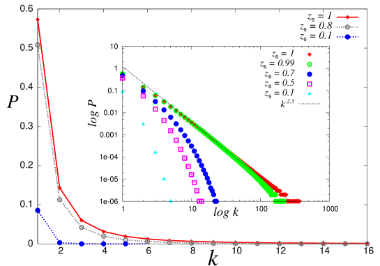
Figure 3: The behavior of the occupation probability (35) in non-asymptotic regime. We set $\varepsilon_{0}=1$ and $z_{s}$ as $z_{s}=0.1,0.8,1.0$, and the inverse temperate is $\beta=1$. The inset of the figure shows the asymptotic behavior of the occupation probability $P(k)$ as Log-Log plots for the cases of $z_{s}=0.1,0.5,0.7,0.99$ and $1$.

We plot the behavior of the occupation probability $P(k)$ in finite $k$ regime in Figure 3. In this plot, we set $\varepsilon_{0}=1$ and $z_{s}$ as $z_{s}=0.1,0.8,1.0$, and the inverse temperate is $\beta=1$. In the inset of the same figure, we also show the same data in Log-Log scale for the asymptotic behavior of the probability $P(k)$ for several values of $z_{s}$, namely, $z_{s}=0.1,0.5,0.7,0.99$ and $1$. From this figure, we find that the power-law $k^{-5/2}$ emerges when the condensation is taken place for $\rho>\rho_{\rm c}$. The numerical analysis of the occupation probability (35) in the limit of $k\to\infty$ is easily confirmed by asymptotic analysis of equation (35). We easily find that the asymptotic form of the wealth distribution $P(k)$ behaves as

$$P(k)=\beta^{-3/2}z_{s}^{k}(1-z_{s})\varepsilon_{0}\Gamma(3/2)\,k^{-3/2}+\frac{3}{2}\beta^{-3/2}z_{s}^{k+1}\varepsilon_{0}\Gamma(3/2)\,k^{-5/2}+{\cal O}(k^{-7/2}).$$ (36)

We also should notice that a macroscopic number of balls $k_{*}$ is gathered to a specific urn with energy level $\epsilon=0$ when the condensation occurs. As the result, the term such as $\sim\,(1/N)\delta(k-k_{*})$ should be added to the occupation probability.

Let us summarize the results as follows:

$$P(k) = \left\{\begin{array}[]{lc}\frac{\varepsilon_{0}(1-z_{s})}{\beta^{3/2}}\,k^{-3/2}\,{\exp}\left[-k\log(1/z_{s})\right]&(\rho<\rho_{\rm c}:z_{s}<1),\\ \frac{3\varepsilon_{0}\Gamma(3/2)}{2\beta^{3/2}}\,k^{-5/2}+\frac{1}{N}\delta(k-k_{*})&(\rho\geq\rho_{\rm c}:z_{s}=1).\end{array}\right.$$ (39)

The scenario of the condensation is as follows. For a given $\rho<\rho_{\rm c}$, one can find a solution $z_{s}<1$ for the saddle point equation (29), and hence the second term of equation (29) is zero in the thermodynamic limit. Then, for non-condensed $N\rho$ balls, the occupation probability follows $\sim\,k^{-3/2}\,{\rm e}^{-k}$-law. Namely, urns possessing a large number of balls do not appear due to the repulsive force as $E=\epsilon n$. When $\rho>\rho_{\rm c}$, the saddle point $z_{s}$ is fixed as $z_{s}=1$; if $z_{s}>1$, the first term of the saddle point equation (29) has a singularity. Therefore, in order to avoid the singularity, the second term of the saddle point equation (29) becomes from zero to a finite value. As the result, the occupation probability is described by the $k^{-5/2}$-law with a delta peak which corresponds to an urn of $\epsilon=0$ gathering the condensed $N(\rho-\rho_{\rm c})$ balls. This corresponds to the condensation phenomena in the disordered urn model. In particular, the occurrence of the condensation in the disordered urn model treated in the present paper is characterized by the transition from the exponential-law to the heavy tailed power-law. We also mention the effect of disorder on the power-law behavior of the occupation probability. We easily find that the power-law behavior disappears when one cancels the disorder of the system by choosing the density of the energy such as $D(\epsilon)=\delta(\epsilon-\hat{\epsilon})$ ($\hat{\epsilon}$ is a constant). This fact means that the disorder appealing in the system possesses a central role to make the occupation probability to have a power-law behavior.

We should notice that in the above argument, the solution $z_{s}=1$ that indicates the condensation does not change even if we choose the density as $D(\epsilon)=\varepsilon_{0}\epsilon^{\alpha},\,(\alpha\geq 0)$. For this choice, the $\rho_{\rm c}$ is given by

$$\rho_{\rm c} = \varepsilon_{0}\beta^{-1-\alpha}\int_{0}^{\infty}\frac{x^{\alpha}dx}{{\rm e}^{x}-1}.$$ (40)

Then, one obtains the following occupation probability

$$P(k) = \frac{z_{s}^{k}\varepsilon_{0}\Gamma(\alpha+1)}{\beta^{\alpha+1}}k^{-\alpha-1}-\frac{z_{s}^{k+1}\varepsilon_{0}\Gamma(\alpha+1)}{\beta^{\alpha+1}}(k+1)^{-\alpha-1}.$$ (41)

At the end of this section, we should mention the result for the uniform distribution of $\epsilon$, that is, the case of $\alpha=0$ leading to $D(\epsilon)=\Theta(\epsilon)-\Theta(\epsilon-1)$. For this choice, we have the following occupation probability

$$P(k) = \frac{z_{s}^{k}}{\beta k}(1-{\rm e}^{-\beta k})-\frac{z_{s}^{k+1}}{\beta(k+1)}(1-{\rm e}^{-\beta(k+1)}).$$ (42)

Then, beyond the critical density $\rho_{\rm c}=\int_{0}^{1}d\epsilon/({\rm e}^{\beta\epsilon}-1)=\beta^{-1}\sum_{n=1}^{\infty}(1-{\rm e}^{-\beta n})/n$, the occupation probability $P(k)$ behaves as

$$P(k) = \frac{\beta^{-1}}{k(k+1)}+\beta^{-1}\left(\frac{k{\rm e}^{-\beta}-k-1}{k(k+1)}\right){\rm e}^{-\beta k}.$$ (43)

Therefore, after the condensation, the crossover from the $k^{-1}{\rm e}^{-\beta k}$-law to the $k^{-2}$-law is observed around $k\sim\beta^{-1}$ and as the result, the power-law heavy tail appears.

5 Interpretation from a view point of macro economics

In this section, we reconsider the results obtained in the previous sections from a view point of macro economics. It is easy for us to regard the occupation probability as wealth distribution when we notice the relations: balls - money and urns - people in a society. In following, we attempt to find an interpretation of the condensation and the emergence of the Pareto-law [22] in terms of wealth differentials [23, 24, 25, 26, 27, 28, 29, 30, 31].

In section 3, we devoted our analysis to extremely large income regimes (the tail of the wealth distribution), however, it is quite important for us to consider the whole range of the wealth. As reported in [30], the wealth distribution for small income regime follows the Gibbs/Log-normal law and a kind of transition to the Pareto-law phase is observed. For the whole range distribution of the wealth, the so-called Lorentz curve [32, 33, 34] is obtained. The Lorentz curve is given in terms of the relation between the cumulative distribution of wealth and the fraction of the total wealth. Then, the so-called Gini index [32, 33, 34, 35], which is a traditional, popular and one of the most basic measures for wealth differentials, could be calculated. The index could be changed from $0$ (no differentials) to $1$ (the largest differentials). For the energy function (26) in the previous section, we derived the wealth distribution for the whole range of incomes $k$. In this section, we evaluate the Gini index analytically.

As we mentioned above, the Lorentz curve is determined by the relation between the cumulative distribution of wealth $X(t)=\int_{t_{\rm min}}^{t}P(k)dk$ and the fraction of the total wealth $Y(t)=\int_{t_{\rm min}}^{t}kP(k)dk/\int_{t_{\rm min}}^{\infty}kP(k)dk$ for a given wealth distribution $P(k)$. For instance, the Lorentz curve for the exponential distribution $P(k)=\gamma\,{\rm e}^{-\gamma k}$ is given by

$$Y = X+(1-X)\log(1-X).$$ (44)

We should notice that the Lorentz curve for the exponential distribution is independent of $\gamma$.

For the power-law distribution $P(k)=(\gamma-1)\,k^{-\gamma}\,\,(\gamma>1)$, we have

$$Y = 1-(1-X)^{\frac{\gamma-2}{\gamma-1}}.$$ (45)

as the Lorentz curve. This curve depends on the exponent $\gamma$. In Figure 4, we plot the Lorentz curve for the exponential distribution (44) and the power-law distribution (45) with several values of $\gamma$.

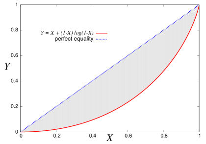
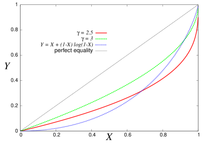
Figure 4: The left panel: The Gini index is obtained as an area between the perfect equality line $Y=X$ and the Lorentz curve (e.g. $Y=X+(1-X)\log(1-X)$ for exponential distributions). The right panel shows the Lorentz curves for the exponential distribution (44) and the power-law distributing (45) with several values of $\gamma=2.5$ and $3$.

Then, as shown in the left panel of Figure 4, the Gini index $G$ is defined as an area between the perfect equality line $Y=X$ and the Lorentz curve. This quantity explicitly reads

$$G = 2\int_{0}^{1}(X-Y)dX=2\int_{t_{\rm min}}^{\infty}(X(t)-Y(t))\cdot\frac{dX}{dt}dt$$ (46)

and we have $G=1/2$ [33, 34] for the exponential distribution and $G=1/(2\gamma-3)$ for the power-law distribution. As the occupation probability distribution (35) is defined for $k>1$, one can evaluate the Gini index as a function of the saddle point $z_{s}$. In Figure 5, we plot the Lorentz curve (left) for several values of $z_{s}$. In the right panel, the Gini index $G(z_{s})$ is shown. We find that the index approaches to $1/2$ as $z_{s}\to 1$.

From the argument in the previous section, we easily find that the occupation distribution for $N\rho_{\rm c}$ non-condensed balls beyond the critical point is modified such as $\sim\,k^{-(\alpha+2)}$ by choosing the density of the energy $D(\epsilon)=\varepsilon_{0}\,\epsilon^{\alpha}$. Namely, for the Pareto-law distribution $\sim k^{-(\alpha+2)}$, the Gini index leads to $G=1/(2\alpha+1)$. Therefore, the condensation is specified by the change of the Gini index from $G=1/2$ to $1/(2\alpha+1)$. However, we should keep in mind that the Gini index itself has less information about the differentials than the wealth distribution. For example, the Gini index for $\alpha=1/2$ of the Pareto-law $P(k)\sim k^{-(\alpha+2)}$ gives the same Gini index as the exponential distribution. This fact stems from the definition of the Gini index $G$, that is, $G$ is defined as an area between $Y=X$ and the Lorentz curve. It could be possible to draw lots of the Lorentz curves that give the same area (the same Gini index). As we explained above, it should be noted that actually the Gini index is one of the measure for the earning differentials, however, the wealth distribution is much more informative than the Gini index.

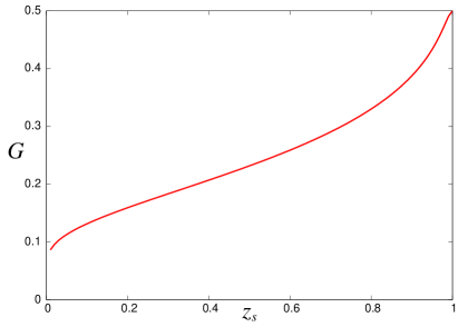
Figure 5: The left panel: the Lorentz curve for (35). The right panel shows the Gini index for several values of $z_{s}$.

Although the Gini index is less informative than the distribution, however, for a given real (empirical) data $x_{1}\leq x_{2}\leq\cdots\leq x_{N}$ ($x$ denotes the amount of money for example. Such empirical data are not always massive enough for us to specify the distribution), one can evaluate it as a statistics by $G=(1/N^{2}\mu)\sum_{i=1}^{N}(2i-N-1)x_{i}$ with $\mu N=\sum_{r=1}^{N}x_{r}$ [35]. Therefore, it is helpful for us to use the Gini index to compare the earning differentials between different countries (the population of each country should be different and of course it is finite $N<\infty$). In our analysis of this paper, the distribution was analytically obtained in the thermo-dynamic limit because we treated an ideal case as a society. Nevertheless, even if we encounter more realistic situation for which the analytical evaluation of wealth distribution is very tough, one can evaluate the earning differentials via the Gini index by computer simulations for finite population $N$. Then, one can investigate the earning differentials by comparing the numerical results with the analytical expressions obtained in this paper.

6 Summary

In this paper, we investigated equilibrium properties of disordered urn model and discuss the condition on which the heavy tailed power-law appears in the occupation probability by using statistical physics of disordered spin systems. We applied our formalism to two urn models of both the Ehrenfest and Monkey classes. In particular, for the choice of the energy function as $E(\epsilon,n)=\epsilon n$ with density of state $D(\epsilon)=\varepsilon_{0}\epsilon^{\alpha}$ for the Monkey class urn model, we found that above the critical density $\rho>\rho_{\rm c}$ for a temperature, the condensation phenomenon is taken place, and most of the balls falls in an urn with the lowest energy level. As the result, the occupation probability changes its scaling behavior from the exponential $k^{-(\alpha+1)}\,{\rm e}^{-k}$-law to the $k^{-(\alpha+2)}$ power-law in large $k$ regime. We also provided a possible link between our results and macro economy, in particular, wealth differentials.

Of course, there might exist the other urn models showing the power-law behavior after the condensation. In fact, we find such a case in a recent study on the Ehrenfest urn model [17], in which the occupation probability follows a Poisson-law when the condensation occurs. Although we provided a piece of evidence to show that the power-law behavior in the occupation probability distribution takes place after the condensation for several restricted cases of the cost function, it is not yet clear whether the condensation always causes the power-law or not. The nature of the link between them will be a central problem to be clarified in future. Therefore, as one of our future studies, it might be important to investigate the universality class of urn models that shows the power-law behavior in the occupation probability beyond the critical point.

We hope that various versions and extensions of the disordered urn model, including Backgammon model [20, 19], could be applied to research area beyond conventional statistical physics.

References

References

- [1] Sherrington D and Kirkpatrick S 1975 Phys. Rev. Lett. 32 1792
- [2] Nishimori H 2001 Statistical Physics of Spin Glasses and Information Processing: An Introduction (Oxford: Oxford University Press)
- [3] Coolen A.C.C 2006 The Mathematical Theory Of Minority Games: Statistical Mechanics Of Interacting Agents (Oxford Finance) (Oxford: Oxford University Press)
- [4] Mezard M, Parisi G and Virasoro M A 1987 Spin Glass Theory and Beyond (Singapore: World Scientific)
- [5] Ehrenfest P and Ehrenfest T 1907 Phys. Zeit. 8 311
- [6] Kac M 1959 Probability and Related Topics in Physical Science, (London: Interscience Publishers)
- [7] Huberman B A and Adamic L A 1999 Nature 401 131
- [8] Barabsi A-L and Albert R 1999 Science 286 509
- [9] Mantegna R N and Stanley H E 2000 An Introduction to Econophysics: Correlations and Complexity in Finance (Cambridge: Cambridge University Press)
- [10] Bouchaud J-P and Potters M 2000 Theory of Financial Risk and Derivative Pricing (Cambridge: Cambridge University Press)
- [11] Scalas E, Martin E and Germano G 2007 Phys. Rev. E 76 011104
- [12] Godreche C and Luck J M 2001 Eur. Phys. J. B. 23 473
- [13] Evans M R and Hanney T 2005 J. Phys. A: Math. Gen. 38 R195
- [14] Ohkubo J, Yasuda M and Tanaka K 2006 Phys. Rev. E 72 065104 (R)
- [15] Ohkubo J, Yasuda M and Tanaka K 2006 J. Phys. Soc. Jpn. 75 074802; Erratum: 2007 ibid. 76 048001
- [16] Ohkubo J 2007 J. Phys. Soc. Jpn. 76 095002
- [17] Ohkubo J 2007 Phys. Rev. E. 76 051108
- [18] Bialas P, Burda Z and Johnston D 1997 Nucl. Phys. B 493 505
- [19] Leuzzi L and Ritort F 2002 Phys. Rev. E 65 056125
- [20] Ritort F 1995 Phys. Rev. Lett. 75 1190
- [21] Morse P M and Feshbach H 1953 Models of theoretical physics (New York: McGraw-Hill, New York)
- [22] Pareto V 1897 Cours d’ Economie Politique Vol. 2 ed Pichou F (Lausanne: University of Lausanne Press)
- [23] Angle J 1986 Social Forces 65 293
- [24] M. Lvy and S. Solomon, Int. J. Mod. Phys. C 7, 65 (1996).
- [25] Ispolatov S, Krapivsky P L and Redner S 1998 Eur. Phys. J. B 2 267
- [26] Bouchaud J-P and Mezard M 2000 Physica A 282 536
- [27] Drgulescu A and Yakovenko V M 2000 Eur. Phys. J. B 17 723
- [28] Chatterjee A, Chakrabarti B K and Manna S S 2003 Physica Scripta 106 36
- [29] Fujiwara Y, DiGuilmi C, Aoyama H, Gallegati M and Souma W 2004 Physica A 335 197
- [30] Chatterjee A, Yarlagadda S and Chakrabarti B K (Eds.) 2005 Econophysics of Wealth Distributions (New Economic Window) (Berlin: Springer)
- [31] Burda Z, Johnston D, Jurkiewicz J, Kaminski M, Nowak M A, Papp G and Zahed I 2002 Phys. Rev. E 65 026102
- [32] Kakwani N 1980 Income Inequality and Poverty (Oxford: Oxford University Press)
- [33] Drgulescu A and Yakovenko V M 2001 Eur. Phys. J. B 20 585
- [34] Silva A C and Yakovenko V M 2005 Europhys. Lett. 69 304
- [35] Sazuka N and Inoue J 2007, Physica A 383 49