Abstract

Collisionless energy absorption in 1D nanoplasma layer is considered. Straightforward classical calculation of the absorption rate in action-angle variables is presented. In regular regime the result obtained is the same as in [4], but deeper insight is possible now due to the technique used. Chirikov criterion of the chaotic absorption regime is written out. Collisionless energy absorption rate in nanoplasma layer is calculated in stochastic regime.

pacs  51.60.+a, 78.20.-e, 52.38.Dx

1 Collisionless absorption in regular regime.

One of the novel problems of laser-matter interaction is the problem of energy absorption in nanometer targets subjected to an ultrashort (up to few picosecond) intence ($10^{13}-10^{17}\mbox{W/cm}^{2}$) laser fields. During such interaction hot (up to several keV energy) classical plasma bounded in nanoscale volume is produced, which has a life time of about hundreds of femtoseconds. This is dense plasma with the electron density of $10^{23}\mbox{cm}^{-3}$ and more. Such systems are used to be called nanoplasma since first experiments of intense short laser interaction with three-dimensional nanobodies (atomic Van-der-Vaals clusters) were hold in 1996 [1].

Nanobodies are known to absorb much more compared to traditional targets like gas or even bulk. The great amount of energy contained in tiny volume results in breakdown, birth of energetic particles and high harmonics generation [2, 3]. Different mechanisms of absorption were suggested to explain such phenomena. They are inner ionization, inverse bremsstrahlung effect, vacuum heating, collisionless heating and some others a bit more sophisticated.

As far as nanoplasma is a strongly bounded system with the width much less than laser wave length, the most interesting mechanism of energy absorption in it is collisionless heating in self-consistent potential. It was considered recently in one-dimensional systems corresponded to irradiated films and more deeply in three-dimesional systems which correspond to nanoclusters; the important role of it in the absorption process was evidently shown (for 1D situation see [4]).

The problem of collisionless energy absorption in thin films irradiated by intence short laser pulse was considered in [4] in the frames of the following model. First, the incompressible liquid approximation for the electronic cloud was used and both the self-consistent potential and distribution function were taken as if they are known function slowly changing on times of the laser pulse duration. This means that the self-consisted system of Boltsman and Laplace equations was supposed to be solved elsewhere. Then, in [4] dipole aproximation and the perturbation theory on the small parameter of the dimensionless oscillation amplitude of the electron cloud was used. Here we use the same model. The calculation of the rate of collisionless absorption presented in [4] was based on quantum-mechanical approach in quasiclassical limit. Note, that the system considered is classical, and the final result in [4] does not contain Plank constant. Althogh this method is non-contradictory, it hides some classical features of the system. The present paper has the aim to make the same calculation for this system in the frames of classical mechanics and to learn more about it possible behaviour.

Let the particle is bounded in self-consistent potential $U(z)$, with the energy distribution function ${\boldsymbol{\rm F}}(\epsilon)$. Mean absorbed energy is defined as:

$$\overline{q}=\int{\rm d}\epsilon{\boldsymbol{\rm F}}(\epsilon)q(\epsilon),$$ (1)

where $q(\epsilon)$ – is the work of the field over the particle with energy $\epsilon$ in the time unit, averaged with the initial condition for this particle. Due to the shielding effect external

$${\bf E}(t)={\bf E}_{0}\cos(\omega t).$$ (2)

and internal $\mathcal{E}$ laser fields differs, and in the model of incompressible fluid used in [4] there is a relation

$${\mathcal{E}}_{z}={E_{0z}\over{\sqrt{(1-\omega_{\rm p}^{2}/\omega^{2})^{2}+4\Gamma^{2}/\omega^{2}}}},$$ (3)

where $\omega_{\rm p}$ is plasma frequency, $\Gamma$ is the damphing constant, and we direct electric field along $z$-axis.

One-particle Hamilton function of the system considered has the form:

$${\mathcal{H}}(p,z,t)=\frac{p^{2}}{2m_{\rm e}}+U(z)-e{\mathcal{E}_{z}}z\cos(\omega t+\alpha)\equiv{\mathcal{H}}_{0}+V_{\rm int}.$$ (4)

It is convenient to come to the action-angle variables $({\mathcal{I}},\varTheta)$, defined for the non-perturbed system in a standart way [5]:

$${\mathcal{I}}=\frac{1}{2\pi}\oint\sqrt{2m_{\rm e}(\epsilon-U(z))}{\rm d}z,~{}~{}~{}\varTheta=\frac{\partial\mathcal{S}_{\tiny\texttt{g}}(z,{\mathcal{I}})}{\partial{\mathcal{I}}},$$ (5)

where

$$\mathcal{S}_{\tiny\texttt{g}}(z,{\mathcal{I}})=\int\sqrt{2m_{\rm e}(\epsilon({\mathcal{I}})-U(z))}{\rm d}z$$ (6)

is a generating function. Using the expansion of the coordinate $z(t)$ in Fourier series

$$z({\mathcal{I}},\varTheta)=\sum_{n}z_{n}({\mathcal{I}})\cos{n\varTheta},~{}~{}~{}$$

$$\mbox{so that~{}}z({\mathcal{I}},\Theta)\cos\omega t=\sum_{n}z_{n}({\mathcal{I}})[\cos(n\Theta+\omega t)+\cos(n\Theta-\omega t)]$$ (7)

we omit highly oscillating terms. Then Hamilton function looks like

$${\mathcal{H}}({\mathcal{I}},\varTheta)={\mathcal{H}}_{0}({\mathcal{I}})-\frac{e{\mathcal{E}}_{z}}{2}\sum_{s}z_{s}({\mathcal{I}})\cos((2s+1)\varTheta-\omega t),~{}~{}z_{n}\equiv z_{s}.$$ (8)

Slow change of the one-particle distribution function on large time scale is a diffusion in action (energy) space (see, for example, [6]), and may be defined by the Fokker-Plank-Kolmogorov equation

$$\frac{\partial{\boldsymbol{\rm F}}(\epsilon,t)}{\partial t}=\frac{1}{2}\frac{\partial}{\partial\epsilon}{\boldsymbol{\textsc{D}}}(\epsilon)\frac{\partial{\boldsymbol{\rm F}}(\epsilon,t)}{\partial\epsilon}.$$ (9)

Here we first introduce the diffusion coefficient

$${\boldsymbol{\textsc{D}}}=\frac{\langle(\delta{\mathcal{I}})^{2}\rangle_{\texttt{T}}}{{\texttt{T}}},$$ (10)

which is defined on large (ideally infinite) observation time T, and do not depend on it. $\delta{\mathcal{I}}$ is the addition to unperturbed action under the influence of the perturbation in (4). To define it we should write down and solve motion equations:

$$\dot{\mathcal{I}}=-\frac{e{\mathcal{E}}_{z}}{2}\sum_{s}(2s+1)z_{s}({\mathcal{I}})\sin\varPsi$$

$$\dot{\varTheta}=\Omega({\mathcal{I}})-\frac{e{\mathcal{E}}_{z}}{2}\sum_{s}\Omega({\mathcal{I}})z^{\prime}_{s}({\mathcal{I}})\cos\varPsi,~{}~{}~{}~{}~{}\varPsi=(2s+1)\varTheta-\omega t.$$ (11)

Then

$$\delta{\mathcal{I}}_{1}=\frac{e{\mathcal{E}}_{z}}{2}\sum_{s}(2s+1)z_{s}({\mathcal{I}}_{0})\cdot\frac{\cos\beta_{s}t-1}{\beta_{s}},~{}~{}~{}~{}~{}\beta_{s}=(2s+1)\Omega(\epsilon_{0})-\omega,$$ (12)

and finally for the diffusion coefficient (10) we get

$${\boldsymbol{\textsc{D}}}=\frac{e^{2}\mathcal{E}^{2}}{4}\sum_{s}\sum_{r}(2s+1)(2r+1)z_{s}({\mathcal{I}})z_{r}({\mathcal{I}})\frac{\langle(1-\cos\beta_{s}{\textsc{T}})(1-\cos\beta_{r}{\textsc{T}})\rangle_{{\textsc{T}}}}{{\textsc{T}}\beta_{s}\beta_{r}}.$$ (13)

To get the energy gain in regular regime without stochasticisy in such description we should take the formal limit $T\to\infty$, because nothing can change the particle trajectory in collisionless system. During the averaging procedure delta-function and delta-symbol $\delta_{rs}$ appears, and finaly diffusion coefficient in regular regime reads as

$${\boldsymbol{\textsc{D}}}({\mathcal{I}})=\frac{{\bf e}^{2}\mathcal{E}^{2}}{4}\sum_{s}(2s+1)^{2}z_{s}^{2}({\mathcal{I}})\pi\delta(\beta_{s}).$$ (14)

To obtain energy gain we integrate FPK-equation (9) by parts and come from action to energy we get:

$$q(\epsilon)=\frac{\partial\langle\epsilon\rangle}{\partial t}=\left\langle\frac{\partial{\mathcal{I}}}{\partial t}\frac{\partial\epsilon}{\partial{\mathcal{I}}}\right\rangle=\frac{\partial}{\partial t}\int{\mathcal{I}}~{}{\rm d}{\mathcal{I}}~{}\Omega({\mathcal{I}}){\boldsymbol{\rm F}}({\mathcal{I}}),~{}~{}~{}~{}\mbox{and}~{}~{}~{}~{}~{}~{}~{}~{}~{}~{}~{}~{}~{}~{}~{}~{}~{}~{}~{}~{}~{}~{}~{}~{}~{}~{}~{}~{}~{}~{}~{}$$

$$\frac{\partial\langle\epsilon\rangle}{\partial t}=\frac{1}{2}\int{\mathcal{I}}\Omega({\mathcal{I}})\frac{\partial}{\partial{\mathcal{I}}}{\boldsymbol{\textsc{D}}}({\mathcal{I}})\frac{\partial{\boldsymbol{\rm F}}({\mathcal{I}})}{\partial{\mathcal{I}}}{\rm d}{\mathcal{I}}=-\frac{1}{2}\int{\rm d}{\mathcal{I}}~{}{\boldsymbol{\textsc{D}}}(I)\Omega(I)\frac{\partial{\boldsymbol{\rm F}}({\mathcal{I}})}{\partial{\mathcal{I}}}=$$

$$=-\frac{\omega a\mathcal{E}_{z}^{2}}{8}m_{\rm e}\omega_{\rm p}^{2}\sum_{s}{z_{s}^{2}({\mathcal{I}}_{s})\over|\Omega^{\prime}_{\epsilon}(\epsilon_{s})|}\frac{\partial{\boldsymbol{\rm F}}({\mathcal{I}}(\epsilon_{s}))}{\partial\epsilon}.$$ (15)

This result repeats the result from [4], where it was obtained on the quasiclassical language. The sum over $s$ here means that only the particle at resonant levels

$$\omega=(2s+1)\Omega(\epsilon)$$ (16)

can absorb energy.

2 Chirikov criterion of the stochasticity.

The technic presented in the previous section allows to describe classical motion of the particles in nanoplasma in the region of parameters, where quasiclassical description used in [4] fails. Supposing that the particle has the initial energy close to resonance energy defined by the condition (16), averaging over time (4) we obtain so-called resonant Hamilton function

$${\mathcal{H}}({\mathcal{I}},\varTheta)={\mathcal{H}}_{0}({\mathcal{I}})-\frac{e{\mathcal{E}}_{z}}{2}z_{s}({\mathcal{I}})\cos((2s+1)\varTheta-\omega t),~{}~{}z_{n}\equiv z_{s}.$$ (17)

According to [7] let us carry out one more canonical transformation with the help of generating function

$$\mathcal{G}({\mathcal{I}},\varPsi,t)=-({\mathcal{I}}-{\mathcal{I}}_{s})\frac{\varPsi+\omega t}{2s+1},$$ (18)

with ${\mathcal{I}}_{s}$ – resonant action, corresponded to the resonance energy with the number $s$ from (16). For new $(P,\varPsi)$ and old $({\mathcal{I}},\varTheta)$ variables the following relations are fulfilled

$$P=-\frac{\partial\mathcal{G}}{\partial\varPsi}=\frac{{\mathcal{I}}-{\mathcal{I}}_{s}}{2s+1},~{}~{}~{}\varTheta=-\frac{\partial\mathcal{G}}{\partial{\mathcal{I}}}=\frac{\varPsi+\omega t}{2s+1}$$ (19)

In new variables Hamiltonian (17) has the form

$${\mathcal{H}}(P,\varPsi)=\frac{1}{2}(2s+1)^{2}\Omega_{\epsilon}^{\prime}(\epsilon_{s})\Omega(\epsilon_{s})P^{2}-\frac{e\mathcal{E}_{z}}{2}z_{s}(\epsilon_{s})\cos\varPsi,$$ (20)

where the decomposition on the small deviation from the resonance action is presented. Hamiltonian function (20) describes the nonlinear mathematical pendulum. Chaotic motion begins when the amplitude in action of such a system is greater than the distance between neighbour

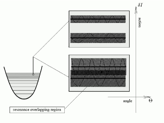
Figure 1: The resonances overlapping.

resonances [7]:

$$\Delta{\mathcal{I}}=\sqrt{\frac{2e\mathcal{E}_{z}z_{s}(\epsilon_{s})}{\left|\Omega_{\epsilon}^{\prime}(\epsilon_{s})\right|\Omega(\epsilon_{s})}}\gtrsim|{\mathcal{I}}(\epsilon_{s})-{\mathcal{I}}(\epsilon_{s+1})|.$$ (21)

This condition means that the action oscillation near one resonance come to the region, occupied by the nearest another one (see Fig.1). The distance between resonances in terms of frequences, according to condition (16) is

$$|\Omega(\epsilon_{s})-\Omega(\epsilon_{s+1})|=\left|\frac{\omega}{2s+1}-\frac{\omega}{2s+3}\right|\approxeq\frac{\omega}{2s^{2}}.$$ (22)

Then, with (21), the criterion of the stochastity appearance, expressed through the field strength inside the system is:

$$\mathcal{E}_{z}\gtrsim\frac{1}{|e|}\left|\frac{\omega^{2}}{8z_{s}(\epsilon_{s})\Omega_{\epsilon}^{\prime}(\epsilon_{s})\Omega(\epsilon_{s})s^{4}}\right|.$$ (23)

This is overestimation: when the inequality is fulfilled, chaos has to take place. In reality threshold is lower [7]. For model potentials from (23) one can find that in rectangular well of the 100 nm width chaotic regime begins if the inner field (3) is about $10^{15}\mbox{W/cm}^{2}$.

3 Collisionless absorption in stochastic regime.

In the situation when chaotic behaviour is developed, to calculate the heating rate in (13) it is nesessary to use for averaging not infinite time, but such a time $\tau_{c}$ which define the dynamical memory of the particle about its previous history. The standart procedure to find it is to define mapping of angle variable [8], which in our system is

$$\Theta_{\mathfrak{n}+1}=\Theta_{\mathfrak{n}}+\frac{2\pi\Omega(\epsilon)}{\omega}+{\mathcal{K}}\sum_{s}\chi_{s}\sin((2s+1)\Theta_{\mathfrak{n}}+\alpha_{s}),$$ (24)

where

$${\mathcal{K}}=\sum_{s}\sqrt{{\mathcal{A}}_{s}^{2}+{\mathcal{B}}_{s}^{2}},~{}~{}~{}~{}~{}~{}\chi_{s}=\sqrt{{\mathcal{A}}_{s}^{2}+{\mathcal{B}}_{s}^{2}}/\sum_{s}\sqrt{{\mathcal{A}}_{s}^{2}+{\mathcal{B}}_{s}^{2}},\\ \alpha_{s}=\frac{(2s+1)\pi\Omega}{\omega}\arccos\left[\frac{{\mathcal{B}}_{s}}{\sqrt{{\mathcal{A}}_{s}^{2}+{\mathcal{B}}_{s}^{2}}}\right],\\ {\mathcal{A}}_{s}=-\frac{e\mathcal{E}_{z}}{\omega-(2s+1)\Omega}\left(\left(\frac{\partial z_{s}({\mathcal{I}})}{\partial{\mathcal{I}}}+\frac{z_{s}(2s+1)}{\omega-(2s+1)\Omega}\frac{\partial\Omega}{\partial{\mathcal{I}}}\right)\sin((2s+1)\pi\Omega/\omega)\right.+\\ \left.+\frac{z_{s}(2s+1)\pi\cos((2s+1)\pi\Omega/\omega)}{\omega}\frac{\partial\Omega}{\partial{\mathcal{I}}}\right)\\ {\mathcal{B}}_{s}=\frac{e\mathcal{E}_{z}}{\omega-(2s+1)\Omega}\frac{3\pi(2s+1)z_{s}\sin((2s+1)\pi\Omega/\omega)}{\omega}\frac{\partial\Omega({\mathcal{I}})}{\partial{\mathcal{I}}}.$$ (25)

For the step time of mapping (24) the period of external laser field was taken. For such mapping the decorellation time $\tau_{c}$ can be estimated as [8]

$$\tau_{c}\simeq\frac{4\pi}{\Delta s~{}\omega\ln{\mathcal{K}}},$$ (26)

where $\Delta s$ is the number of essential items $\chi_{s}$ in sum (24). In our situation it has the order of $2s+1$. Finally, the diffusion coefficient can be obtained from (13) with substitution ${\textsc{T}}\rightarrow\tau_{c}$. It reads

$${\boldsymbol{\textsc{D}}}({\mathcal{I}})=\frac{e^{2}\mathcal{E}^{2}}{4}\sum_{s}\sum_{r}(2s+1)(2r+1)z_{s}({\mathcal{I}})z_{r}({\mathcal{I}})\Delta_{rs}(\tau_{c}),$$ (27)

where

$$\Delta_{rs}(\tau)=\frac{(1-\cos\beta_{s}\tau)(1-\cos{\beta_{r}\tau})}{\tau\beta_{s}\beta_{r}}.$$ (28)

Energy gain can be obtained from the FPK-equation in the same way as we did it earlier for regular regime (15):

$$\frac{\partial\langle\epsilon\rangle}{\partial t}={\boldsymbol{\textsc{D}}}({\mathcal{I}})=\frac{e^{2}\mathcal{E}^{2}}{4}\int{\rm d}\epsilon\Omega(I(\epsilon))\frac{\partial{\boldsymbol{\rm F}}({\mathcal{I}}(\epsilon))}{\partial\epsilon}\sum_{sr}(2s+1)(2r+1)z_{s}({\mathcal{I}}(\epsilon))z_{r}({\mathcal{I}}(\epsilon))\Delta_{rs}(\epsilon,\tau_{c}).$$ (29)

In this expression all resonance levels take part in the absorption process simultaneously. Moreover, in such a situation particle with arbitrary energy should gain energy from the external field. Formula (29) is the main result of the present work. It describes the collisionless heating in 1D classical nanoplasma layer when the field strength is enough for chaotic regime to take place, according to (23).

Author wishes to thank S.V. Popruzhenko, D.F. Zaretsky, I.Yu. Kostyukov for fruitful discussions. The work was done with the financial support of RFBR.

References

• [1] T. Ditmire, T. Donnelly, A. M. Rubenchik, R. W. Falcone, and M. D. Perry, Phys. Rev. A 53, 3379 (1996), Y. L. Shao, T. Ditmire, J. W. G. Tisch, E. Springate, J. Marangos, and M. H. R. Hutchinson, Phys. Rev. Lett. 77, 3343 (1996)
• [2] Jasapara J., Nampoothiri A. V. V., Rudolph W., Ristau D., Starke K., 2001, Phys. Rev.B 63, 045117
• [3] Tom H.W.K., Wood O.R.II, Aumiller G.D., Rosen M.D. In: Springer series in chemical physics, Ultrafast phenomena VII (Berlin, Heidelberg, Springer-Verlag, 1990, v.53, p.107-109).
• [4] D.F. Zaretsky, Ph.A. Korneev, S.V. Popruzhenko and W. Becker, Journal of Physics B: Atomic, Molecular and Optical Physics, V. 37, 4817-4830, 2004.
• [5] Landau L D and Lifshitz E M 1979 Mechanics. (Oxford: Pergamon)
• [6] Regular and Chaotic Dynamics, 2nd Edition; A.J. Lichtenberg, M.A. Lieberman, Springer Verlag, 1992
• [7] Chirikov B.V., Phys. Reports, Vol.52, p.265 (1979)
• [8] G.M. Zaslavsky, ”Stochasticity of the dynamical systems”, Moscow, ”Nauka”, 1984 (in russian).