Axially symmetric focusing as a cuspoid diffraction catastrophe:
Scalar and vector cases and comparison with the theory of Mie

Abstract

An analytical description of arbitrary strongly aberrated axially symmetric focusing is developed. This is done by matching the solution of geometrical optics with a wave pattern which is universal for the underlying ray structure. The corresponding canonical integral is the Bessoid integral, which is a three-dimensional generalization of the Pearcey integral that approximates the field near an arbitrary two-dimensional cusp. We first develop the description for scalar fields and then generalize it to the vector case. As a practical example the formalism is applied to the focusing of light by transparent dielectric spheres with a few wavelengths in diameter. The results demonstrate good agreement with the Mie theory down to Mie parameters of about 30. Compact analytical expressions are derived for the intensity on the axis and the position of the diffraction focus both for the general case and for the focusing by microspheres. The high intensity region is narrower than for an ideal lens of the same aperture at the expense of longitudinal localization and has a polarization dependent fine structure, which can be explained quantitatively. The results are relevant for aerosol and colloid science where natural light focusing occurs and can be used in laser micro- and nano-processing of materials.

I Introduction

Axially symmetric focusing of wave fields occurs in various areas of science, since physical systems often possess an intrinsic rotational symmetry. In particular, the electromagnetic field enhancement by small spherical particles is important in many situations. Spheres have minimal surface energy for a given volume and thus are naturally formed as a result of phase separation, for example as aerosols or colloids. Applications of colloidal microspheres in photonic crystals and photonic crystal slabs led to an explosion of the experimental and theoretical studies of their optical properties.Wij1998 ; Vla2001 The majority of these investigations concentrate on their collective properties in a periodic arrangement. Single microspheres are used as high quality optical resonators and as agents that allow controlled and highly localized wavelength-dependent field enhancement for non-linear optical studies and in resonance spectroscopy.Gor1996 ; Vah2003 Here, the emphasis is placed on the eigenmode analysis and the distribution of the field within the sphere or in the immediate vicinity of its surface.

Lately, it was demonstrated that self-assembling arrays of transparent colloidal microspheres can be employed for high-throughput laser-assisted micro- and nano-structuring of materials.Bur1999 ; Bae2000 ; Bae2004 Similar effects were observed in experiments on dry laser cleaning, where such particles are used as controlled contaminants.Mue2001 ; Luk2002 ; Luk2003 This necessitates better understanding of the focusing of light by microspheres with diameters of several wavelengths. Only few rigorous results are available for the intermediate range of sphere sizes and distances from the particle. The majority of analytical approaches either deal with the properties of the eigenmodes, or refer to the integral characteristics and/or to the far field behavior.Boh1983 Mie resonances were analyzed on the basis of advanced geometrical opticsRol2000 and detailed numerical calculations for transparent spheres of several wavelengths in size were performed in connection with the use of laser tweezers in biologyRoh2005 and for needs of aerosol science.Zim2001

In this work we develop a theoretical description for an arbitrary non-paraxial strongly aberrated axially symmetric focusing and apply it to the case of dielectric microspheres. Our emphasis is on the fine structure of the field distribution in the exterior of the sphere up to the focal region, which can be used to control and improve the concentration of energy.

Strong spherical aberration makes the focusing non-trivial. Usually, the exact solution is obtained using the Mie theory,Mie1908 which does not give much of a physical insight as it requires the summation of a large number of terms in a multipole expansion even for moderate sphere sizes. At the same time, the main focusing properties of transparent dielectric microspheres originate rather from the picture of geometrical optics.

One might think that in the lowest approximation a small sphere acts as an ideal lens. However, in the range of sizes we are interested in, this picture does not even provide a description which is qualitatively correct. Also classical formulas for weak spherical aberration Bor2002 do not yield useful results for the field behind a sphere: They predict that the maximum intensity is kept unchanged and its position does not depend on the wavelength.

Our approach, following the method of uniform caustic asymptotics,Kra1999 is based on the canonical integral for the cuspoid ray topology of strong spherical aberration. Though this Bessoid integral — a member of the hierarchy of diffraction catastrophesBer1980 ; Ber2001a — appears naturally in the paraxial approximation, it can be used to describe arbitrary axially symmetric strong spherical aberration by appropriate coordinate and amplitude transformations. For angularly dependent vectorial amplitudes the formalism uses higher-order Bessoid integrals.

The Bessoid integral is the axially symmetric generalization of the Pearcey integral,Pea1946 which plays an important role in many short wavelength phenomena.Con1981 Therefore, the present approach can be applied in various areas of physics where axially symmetric focusing is of importance, e.g., acoustics, semiclassical quantum mechanics, radio wave propagation and scattering theory.

II The Bessoid integral

II.1 Definition

We first consider the diffraction of a scalar spherically aberrated wave on a circular aperture with radius $a$ in the plane $z=-f$ around the $z$-axis, where $f$ is the focal distance. The origin of the coordinate system is put into the focus $F$. In cylindrical coordinates $(\rho,z)$, the paraxial Fresnel–Kirchhoff diffraction integral Bor2002 yields the field amplitude

$$U(\rho,z) =-\dfrac{\text{i}\,k\,U_{0}}{f}\;\text{e}^{\,\text{i}\,k\,z}$$

$$\;\;\times\int\nolimits_{0}^{a}J_{0}\!\left(k\,\dfrac{\rho\,\widetilde{\rho}_{1}}{f}\right)\text{e}^{-\,\text{i}\,k\,\tfrac{z\,\widetilde{\rho}_{1}^{2}}{2\,f^{2}}\,-\,\text{i}\,k\,B\,\widetilde{\rho}_{1}^{4}}\,\widetilde{\rho}_{1}\,\text{d}\widetilde{\rho}_{1}.$$ (1)

Here $U_{0}$ is the amplitude of the incident wave in the center of the aperture, $k$ is the wavenumber ($k=2\pi/\lambda$, where $\lambda$ is the wavelength) and $\widetilde{\rho}_{1}$ is the distance from the axis on the aperture. The Bessel function $J_{0}$ comes from the integration over the polar angle $\varphi$. The parameter $B$ in the exponent determines the strength of the spherical aberration. For $B>0$ the diffraction focus shifts towards the aperture, while $B=0$ corresponds to ideal focusing.Bor2002

We introduce the dimensionless coordinates $\rho_{1}\equiv\sqrt[4]{4\,k\,B}\,\widetilde{\rho}_{1}$, $R\equiv\sqrt[4]{k^{3}/4\,B}\,\rho/f$ and $Z\equiv\sqrt{k/4\,B}\,z/f^{2}$ and consider an infinitely large aperture. Then the field (1) becomes proportional to the Bessoid integral Kir2000

$$I(R,Z) ={\displaystyle\int\nolimits_{0}^{\infty}}\rho_{1}\,J_{0}(R\,\rho_{1})\;\text{e}^{-\,\text{i}\,\left(Z\,\tfrac{\rho_{1}^{2}}{2}\,+\,\tfrac{\rho_{1}^{4}}{4}\right)}\text{d}\rho_{1}$$ (2)

$$=\dfrac{1}{2\,\pi}\int\nolimits_{-\infty}^{\infty}\int\nolimits_{-\infty}^{\infty}\text{e}^{\,\text{i}\,\phi}\,\text{d}x_{1}\text{d}y_{1},$$ (3)

where

$$\phi\equiv-R\,x_{1}-Z\,\dfrac{x_{1}^{2}+y_{1}^{2}}{2}-\dfrac{(x_{1}^{2}+y_{1}^{2})^{2}}{4}\,.$$ (4)

Its absolute square is shown in figure 1. In the Cartesian representation $x_{1}=\rho_{1}\cos\varphi$ and $y_{1}=\rho_{1}\sin\varphi$ are dimensionless coordinates in the plane of integration. Expression (3) is the axially symmetric generalization of the Pearcey integral Pea1946

$$I_{P}(X,Z)=\dfrac{1}{\sqrt{2\,\pi}}\,{\displaystyle\int\nolimits_{-\infty}^{\infty}}\,\text{e}^{-\,\text{i}\,\left(X\,x_{1}\,+\,Z\,\tfrac{x_{1}^{2}}{2}\,+\,\tfrac{x_{1}^{4}}{4}\right)}\text{d}x_{1},$$ (5)

which is also shown in figure 1.

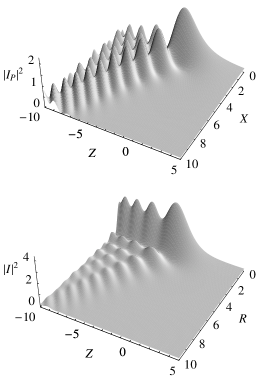
Figure 1: Absolute square of the Pearcey integral $I_{P}$ (top) and the Bessoid integral $I$ (bottom). The latter is proportional to the field of a spherically aberrated wave within small angles approximation.

Both integrals correspond to so-called diffraction catastrophes.Kra1999 ; Ber1980 ; Ber2001a Their field distribution contains caustic zones where the intensity predicted by geometrical optics goes to infinity. The Pearcey integral corresponds to a cusp caustic, i.e., a single one-dimensional curve in a two-dimensional space, and does not reveal a high intensity along the axis, while the Bessoid integral corresponds to a cuspoid caustic, i.e., to a surface of revolution of the cusp in three dimensions, as well as the caustic line up to the focus $F$ at $z=Z=0$. The equation of the cusp is given by the semicubic parabola

$$27\,R^{2}+4\,Z^{3}=0\,.$$ (6)

Henceforth we will apply the term cusp also for the whole cuspoid. A caustic is denoted as stable, if it does not change its topology under small perturbations. This is the case for the Pearcey integral. The Bessoid integral corresponds to a structurally unstable caustic, because an infinitely small perturbation will destroy the radial symmetry and the axis will not be a caustic zone any longer. It is, however, stable on the class of axially symmetric wavefronts.

The cusp is the envelope of the family of rays. The latter correspond to the points of stationary phase in the Bessoid integral, i.e., those points where the two first partial derivatives with respect to $R$ and $Z$ of the phase $\phi$ in (3) vanish. Inside the cusp, for $27\,R^{2}+4\,Z^{3}<0$, three rays (tangents to the cusp) arrive at each point of observation $P\equiv(\rho,z)$, and outside, for $27\,R^{2}+4\,Z^{3}>0$, there is only one real ray (figure 2). Thus, the cusp forms the border between the lit region and the (partial) geometrical shadow, where two rays merge.

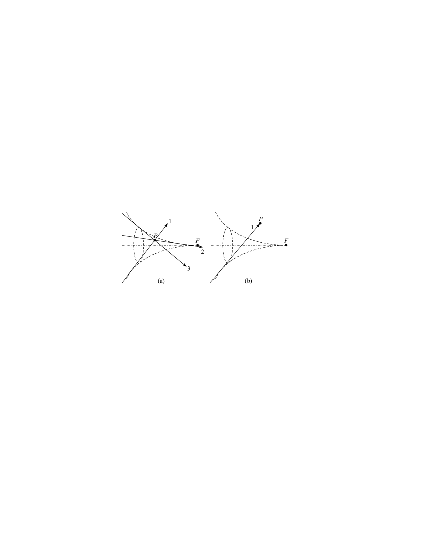
Figure 2: (a) 3-ray region inside the cuspoid (dashed line). (b) 1-ray region outside. The $z$-axis is represented by a dashed-dotted line.

Without loss of generality, we assume that all rays lie in the meridional plane $\varphi=0$ ($y_{1}=0$) and hence correspond to the roots $x_{1,j}$ ($j=1,2,3$) of the cubic equation

$$R+Z\,x_{1}+x_{1}^{3}=0\,,$$ (7)

which are given by Cardan’s formulas.Bro2004 On the axis, $R=0$, a cone formed by an infinite number of rays converges. These rays originate from the circle $x_{1}^{2}+y_{1}^{2}=-Z$ on the aperture. They are all in phase and produce a high intensity along the axis (compare the two pictures in figure 1). The oscillations occur due to interference with the ray propagating along the $z$-axis. One can also directly observe that the Bessoid integral has the topology of spherical aberration as the maximum of intensity does not lie in the geometrical focus $Z=0$ but is spherically aberrated to a negative value of $Z$, i.e., towards the aperture.

II.2 Asymptotic expressions

Off the caustic — away from the cusp and the focal line — the Bessoid integral (3) can be approximated by the method of stationary phase. As the integrand in (3) is highly oscillatory, the only significant contributions to the integral come from those regions where the phase is stationary:Foc1956

$$I(R,Z)\approx{\displaystyle\sum\limits_{j=1}^{m}}\,\dfrac{\text{e}^{\,\text{i}\,\phi_{j}\,+\,\text{i}\,\tfrac{\pi}{4}\,\text{sign}\,\mathbf{H}_{j}}}{\sqrt{\left|\det\mathbf{H}_{j}\right|}}\,,$$ (8)

where the summation runs over all real rays, i.e., $m=1$ (lit region) or $m=3$ (shadow). The phase $\phi_{j}$ is obtained by inserting the $j$-th stationary point $(x_{1,j},y_{1,j}\!=\!0)$ into the (4). The determinant and signature of the Hessian are given by

$$\det\mathbf{H}_{j} =Z^{2}+4\,x_{1,j}^{2}\,Z+3\,x_{1,j}^{4}\,,$$ (9)

$$\text{sign}\,\mathbf{H}_{j} =\text{sgn}(-Z-3\,x_{1,j}^{2})+\text{sgn}(-Z-x_{1,j}^{2})\,.$$ (10)

Near the cusp the Bessoid integral shows an Airy-type behavior typical for caustics where two real rays disappear and become complex.

One can also derive a different approximation valid on and near the caustic axis, i.e., for $Z\leq 0$ and small $R$ (appendix A):

$$I(R,Z)\approx\dfrac{\sqrt{\pi}}{2}\,J_{0}(R\sqrt{-Z})\;\text{e}^{\,\text{i}\,\tfrac{Z^{2}-\pi}{4}}\,\operatorname{erf}\!\text{c\negthinspace}\left(\dfrac{Z}{2}\;\text{e}^{\,\text{i}\,\tfrac{\pi}{4}}\right)\text{\negthinspace}.$$ (11)

Here erfc is the complementary error function,Abr1993 which can also be written in terms of Fresnel sine and cosine functions.Kir2000 Expression (11) becomes exact at the axis $R=0$, where $J_{0}(0)=1$. It shows that near the axis the Bessoid integral is virtually a Bessel beamMcG2005 with a variable cross section.

II.3 Numerical evaluation

As the Bessoid integrand is highly oscillatory, its evaluation for the whole range of coordinates $R$ and $Z$ is non-trivial and of large practical importance. Direct numerical integration along the real axis and the method of steepest descent in the complex plane both have their disadvantages. By far the fastest technique is based on the numerical solution of the ordinary differential equation (derivation in appendix B)Kof2004 ; Time

$$L_{R}-Z\,I_{R}+\text{i}\,R\,I=0\,.$$ (12)

Indices denote (partial) derivatives and $L\equiv I_{RR}+I_{R}/R$ is an abbreviation for the radial Laplacian applied onto $I$. The three initial conditions at $R=0$ are

$$I(0,Z) =\dfrac{\sqrt{\pi}}{2}\;\text{e}^{\,\text{i}\,\tfrac{Z^{2}-\pi}{4}}\,\operatorname{erf}\!\text{c\negthinspace}\left(\dfrac{Z}{2}\;\text{e}^{\,\text{i}\,\tfrac{\pi}{4}}\right)\text{\negthinspace},$$ (13)

$$I_{R}(0,Z) =0\,,$$ (14)

$$L(0,Z) =Z\,I(0,Z)+\text{i}\,.$$ (15)

$I(0,Z)$ was taken from (11), $I_{R}(0,Z)$ vanishes due to symmetry, and the last condition arises from the fact that the Bessoid integral satisfies the paraxial Helmholtz equation $2\,$i$\,I_{Z}+L=0$, where $I_{Z}$ is calculated from (13).

In the literature the Pearcey integral was calculated by solving differential equations,Con1984 by a series representation Con1973 and by the first terms of its asymptotic expansion.Sta1983 The Bessoid integral was expressed in terms of parabolic cylinder functions Jan1992 and as a series.Kir2000 The latter work gives reference to an unpublished work of Pearcey,Pea1963 stating that differential equations for the Bessoid integral were employed there.

II.4 Geometrical optics for the cuspoid

In geometrical optics, the rays carry the information of amplitude and phase. The total field in a point $P$ is given by the sum of all ray fields there. A ray’s field at $P$ is determined byKra1990

$$U(P)=U_{0}\,\dfrac{\text{e}^{\,\text{i}\,k\,\psi}}{\sqrt{J}}\,,$$ (16)

where $U_{0}$ is the amplitude at some initial wavefront, $\psi$ is the eikonal, and $J$ is the generalized geometrical divergence, which can be calculated from flux conservation along the ray. For a homogeneous medium with constant refractive indexKra1990

$$J=\dfrac{R_{m}R_{s}}{R_{m0}R_{s0}}\,.$$ (17)

$R_{m}$, $R_{s}$ are the main radii of curvature at the point $P$ and $R_{m0}$, $R_{s0}$ are the radii on the initial wavefront, where $U=U_{0}$.

When a ray touches a caustic, its radius of curvature (the geometrical divergence in the general case) changes the sign and the ray undergoes a caustic phase delay Kra1990 ; Kra1999  of $-\pi/2$, which is taken into account by the proper choice of the square root in (16). When a ray touches several caustics, these delays must be added. The total caustic phase shift, denoted as $\Delta\varphi$, can be explicitly written in the phase. For the cuspoid topology and ray numbering ($j=1,2,3$) according to figure 2, we obtain:

$$U(P)=U_{0}\,\dfrac{\text{e}^{\,\text{i}\,k\,\psi}}{\sqrt{J}}=U_{0}\,\dfrac{\text{e}^{\,\text{i}\,k\,\psi\,+\,\text{i}\,\Delta\varphi}}{\sqrt{\left|J\right|}}$$ (18)

with

$$\Delta\varphi_{j}=\left\{\begin{array}[c]{rl}-\pi&\text{ for }j=1,\\ 0&\text{ for }j=2,\\ -\pi/2&\text{ for }j=3.\end{array}\right.$$ (19)

Ray 1 touched the cuspoid and the focal line, ray 2 is not shifted, and ray 3 touched the cuspoid.

III Relation between geometrical and wave optics

III.1 Matching with the Bessoid integral

If we have found the phases $\varphi\equiv k\,\psi$ and divergences $J$ of the rays, the (scalar) geometrical optics solution with an axially symmetric 3-ray cuspoid topology can be written as

$$U(\mathbf{r})=\sum_{j=1}^{3}\dfrac{U_{0,j}\;\text{e}^{\,\text{i}\,\varphi_{j}(\mathbf{r})}}{\sqrt{J_{j}(\mathbf{r})}}\,.$$ (20)

Here $\mathbf{r}\equiv(\rho,z)$ are the real-space coordinates and we have allowed for different initial amplitudes $U_{0,j}$ of the rays. This field shows singularities at the caustic, especially on the axis, which is the most interesting region for applications.

We want to describe arbitrary axially symmetric focusing by matching the solution of geometrical optics (where it is correct) with a wave field constructed from the Bessoid integral (3), which naturally appears in the paraxial approximation and is finite everywhere, and its partial derivatives $I_{R}$ and $I_{Z}$ (method of uniform caustic asymptotics). We make the Ansatz Kra1999

$$U=\left(A\,I+\dfrac{1}{\text{i}}\,A_{R}\,I_{R}+\dfrac{1}{\text{i}}\,A_{Z}\,I_{Z}\right)\text{e}^{\,\text{i}\,\chi}\,.$$ (21)

The yet unknown arguments of the Bessoid integral and its derivatives are $\mathbf{R}\equiv(R(\mathbf{r}),Z(\mathbf{r}))$. $A(\mathbf{r})$, $A_{R}(\mathbf{r})$ and $A_{Z}(\mathbf{r})$ are three amplitude factors and $\chi(\mathbf{r})$ is a phase function. (The indices $R$ and $Z$ in the amplitudes do not indicate derivatives.) Now the geometrical optics solution (20) is matched with the stationary phase approximation of (21) by equating the amplitudes and phases:Kra1999 ; Bre1992

$$\dfrac{U_{0,j}}{\sqrt{J_{j}}} =\dfrac{A(\mathbf{r})+A_{R}(\mathbf{r})\,\phi_{R}(\mathbf{R},\mathbf{t}_{j})+A_{Z}(\mathbf{r})\,\phi_{Z}(\mathbf{R},\mathbf{t}_{j})}{\sqrt{H_{j}}}\,,$$ (22)

$$\varphi_{j}(\mathbf{r}) =\chi(\mathbf{r})+\phi(\mathbf{R},\mathbf{t}_{j})\,.$$ (23)

$\phi_{R}$ and $\phi_{Z}$ are the partial derivatives of (4) and

$$\dfrac{1}{\sqrt{H_{j}}}\equiv\dfrac{\text{e}^{\,\text{i}\,\tfrac{\pi}{4}\,\text{sign}\,\mathbf{H}_{j}}}{\sqrt{\left|\det\mathbf{H}_{j}\right|}}\,,$$ (24)

where the determinant and signature of the Hessian are written in (9) and (10), respectively. Outside the cusp, the rays 2 and 3 are complex and the general definition of $H_{j}$ is more subtle, namely

$$\dfrac{1}{\sqrt{H_{j}}}\equiv\sqrt{\dfrac{\text{i}}{\phi_{20,j}}}\,\sqrt{\dfrac{\text{i}}{\phi_{02,j}}}\,,$$ (25)

with $\phi_{20}\equiv\partial^{2}\phi$/$\partial x_{1}^{2}$, $\phi_{02}\equiv\partial^{2}\phi/\partial y_{1}^{2}$ (the index $j$ denotes substitution of the $j$-th point of stationary phase as argument).

The three points of stationary phase were denoted as $\mathbf{t}_{j}\equiv(t_{j},0)$, where the $t_{j}$ are given by the (correctly ordered) Cardan’s solutions of (7), i.e., of

$$R+Z\,t+t^{3}=0\,.$$ (26)

Note that they are functions of the Bessoid coordinates, $\mathbf{t}_{j}=\mathbf{t}_{j}(\mathbf{R})$, and the latter depend on the real space coordinates: $\mathbf{R}=\mathbf{R}(\mathbf{r})$. The partial derivatives with respect to $R$ and $Z$ in (22) must be evaluated in such a way as the $t_{j}$ were held constant, although they are functions of $\mathbf{R}$ themselves. The conditions (22) and (23) give 6 equations for the 6 unknowns $R$, $Z$, $\chi$, $A$, $A_{R}$, and $A_{Z}$.

It is convenient to solve (23), that is

$$\varphi_{j}=\chi-R\,t_{j}-\dfrac{1}{2}\,Z\,t_{j}^{2}-\dfrac{1}{4}\,t_{j}^{4}\,,$$ (27)

using quantities that are permutationally invariant with respect to the roots $t_{j}$.Con1981 ; Bre1992 This yields

$$R =\sqrt{\dfrac{Z^{3}}{54}-\dfrac{4\,b_{2}}{9\,Z}}\,,$$

$$Z =\pm\sqrt[4]{\dfrac{2}{3}}\,\sqrt{-2\,\text{sgn}(b_{3})\,\sqrt{b_{2}+q}+2\,\sqrt{D}}\,,$$ (28)

$$D \equiv 2\,b_{2}-q+2\sqrt{b_{2}^{2}-b_{2}\,q+q^{2}}\,,$$

$$\chi =b_{1}-\dfrac{1}{6}\,Z^{2}\,,$$

where sgn$(Z)=\;$sgn$(Z^{4}-24\,b_{2})$. The $b_{l}$ ($l=1,2,3$) are given by $b_{1}\equiv(1/3)$ ${\textstyle\sum\nolimits_{j=1}^{3}}\varphi_{j}$, $b_{2}\equiv{\textstyle\sum\nolimits_{j=1}^{3}}(\varphi_{j}-b_{1})^{2}$ and $b_{3}\equiv{\textstyle\sum\nolimits_{j=1}^{3}}(\varphi_{j}-b_{1})^{3}$. The quantity $q$ (sometimes called discriminant) can be expressed in different ways:

$$q^{3} \equiv 6\,b_{3}^{2}-b_{2}^{3}=\dfrac{1}{2^{11}}\,R^{2}\,(27\,R^{2}+4\,Z^{3})^{3}$$

$$=-2\,(\varphi_{1}-\varphi_{2})^{2}\,(\varphi_{2}-\varphi_{3})^{2}\,(\varphi_{3}-\varphi_{1})^{2}\,.$$ (29)

Hence, it vanishes exactly at the caustic where two phases are equal. At the cuspoid $\varphi_{2}=\varphi_{3}$ ($27\,R^{2}+4\,Z^{3}=0$) and on the axis $\varphi_{1}=\varphi_{3}$ ($R=0$).

The solutions of (22), that is

$$\dfrac{U_{0,j}}{\sqrt{J_{j}}}=\dfrac{A-t_{j}\,A_{R}-\frac{1}{2}\,t_{j}^{2}\,A_{Z}}{\sqrt{H_{j}}}\,,$$ (30)

areBre1992

$$A =-\,U_{0,1}\,\dfrac{\sqrt{H_{1}}}{\sqrt{J_{1}}}\,\dfrac{t_{2}\,t_{3}}{(t_{3}-t_{1})\,(t_{1}-t_{2})}-...-...\,,$$

$$A_{R} =U_{0,1}\,\dfrac{\sqrt{H_{1}}}{\sqrt{J_{1}}}\,\dfrac{t_{1}}{(t_{3}-t_{1})\,(t_{1}-t_{2})}+...+...\,,$$ (31)

$$A_{Z} =2\,U_{0,1}\,\dfrac{\sqrt{H_{1}}}{\sqrt{J_{1}}}\,\dfrac{1}{(t_{3}-t_{1})\,(t_{1}-t_{2})}+...+...\,,$$

where the cyclic terms permutate the numbering of rays: $(1,2,3)\rightarrow(2,3,1)\rightarrow(3,1,2)$. The Bessoid matching solution (21) does not show the divergences of geometrical optics.

Note that this method utilizes also the so-called complex rays which have less apparent physical meaning. It turns out that both real and complex rays provide the geometrical skeleton for the wave flesh.Kra1999

III.2 Expressions on and near the axis in the general case

All formulas can be strongly simplified on and near the axis inside the cuspoid (small $\rho$, $z<0$). The Bessoid coordinates have the simple form (appendix C)

$$R \approx\dfrac{(\varphi_{1}-\varphi_{3})/2}{\sqrt{2}\,\sqrt[4]{(\varphi_{1}+\varphi_{3})/2-\varphi_{2}}}\approx\dfrac{k\,\rho\,\sin\beta}{\sqrt{-Z}}\,,$$ (32)

$$Z \approx-2\,\sqrt{\dfrac{\varphi_{1}+\varphi_{3}}{2}-\varphi_{2}}\approx-2\,\sqrt{\varphi_{\text{np}}-\varphi_{\text{p}}}\,,$$ (33)

where $\beta>0$ is the local angle of the non-paraxial cone of rays with the axis and $\varphi_{\text{np}}$ and $\varphi_{\text{p}}$ denote the phases of the non-paraxial rays and the (par)axial ray, respectively (see figure 9 in appendix C). The simple natural combination

$$R\sqrt{-Z}\approx\dfrac{\varphi_{1}-\varphi_{3}}{2}\approx k\,\rho\,\sin\beta$$ (34)

also appears in the near axis approximation for the Bessoid integral (11). On the axis ($\rho=0$, $\varphi_{1}=\varphi_{3}$) we obtain $R=0$ and $Z=-2\,\sqrt{\varphi_{1}-\varphi_{2}}$.

The results (32)–(34) have transparent physical meaning. Indeed, near the axis the largest contribution to the field comes from the converging cone of non-paraxial rays (similar to ray 1) that intersect the axis at an angle $\beta$. If the angle $\beta$ is constant and all rays have the same intensity, the result is the Bessel beam.McG2005 Such beams have a propagation constant along the $z$-direction equal to the $z$-component of the wavevector of the plane waves which form them and correspondingly the argument of the Bessel function (cylindrical analog of a plane wave) is equal to $k\,\rho\,\sin\beta$. As the angle $\beta$ gradually changes for the spherically aberrated wave, so does the argument of the Bessel function.

Additionally, there exists the axial ray 2, which is not present in the canonical Bessel beam (though it often appears in real experimental situations). The interference of this beam with the converging ray cone results in the intensity oscillations along the axis (figure 1, bottom). Clearly, these oscillations are largely due to the phase difference $\varphi_{\text{np}}-\varphi_{\text{p}}$. At large negative $Z$ in (11) erfc$[\tfrac{Z}{2}\exp($i$\tfrac{\pi}{4})]\rightarrow 2\,[1\!-\!\tfrac{1}{\sqrt{\pi}\,Z}\exp($i$\tfrac{3\pi-Z^{2}}{4})]$, and the oscillating behavior is governed by the phase of the exponent, which is equal to $3\,\pi/4-(\varphi_{\text{np}}-\varphi_{\text{p}})$. This clarifies the origin of expression (33), as it is $Z^{2}$ entering the final formulas.

In particular, the global maximum is expected on axis at the first constructive interference of the axial and the non-paraxial rays. Because $Z<0$ in this region, the two terms of the erfc expansion are first in phase when the phase difference is $\varphi_{1}-\varphi_{2}=3\,\pi/4$. The geometrical meaning of this result is that rays 1 and 3 are shifted by $-\pi/2$ as they touch the cusp. In addition, they acquire a further shift of $-\pi/2$ when crossing the focal line. But exactly on the axis only half of this delay has occurred yet, which yields the $3\,\pi/4$ difference. The numerical maximum of the Bessoid intensity (absolute square) occurs at $Z_{\text{m}}\approx-3.051$ and hence this yields the condition

$$\varphi_{1}-\varphi_{2}=\dfrac{Z_{\text{m}}^{2}}{4}\approx 2.327\,,$$ (35)

which is close to $3\,\pi/4\approx 2.356$.

The width of the focal line caustic, $\rho_{w}$, is defined by the first zero $w_{0}\approx 2.405$ of the Bessel function in (11). Hence, with (34),

$$\rho_{w}\equiv\dfrac{w_{0}}{k\,\sin\beta}\approx 0.383\,\dfrac{\lambda}{\sin\beta}\,.$$ (36)

In the geometrical optics picture the first minimum occurs when rays 1 and 3 interfere destructively, i.e., when their phase difference becomes $\pi$. This results in $\varphi_{1}-\varphi_{3}=\pi+\pi/2$, where the term $\pi/2$ takes into account the caustic phase shift of ray 1: $\rho_{w}\approx(\varphi_{1}-\varphi_{3})/2\,k\,\sin\beta=0.375\,\lambda/\sin\beta$. Note, that this is smaller than the Airy spot for the same aperture angleBor2002 and large angles $\beta$ are indeed realized, e.g., in the case of the sphere studied below.

Finally, we present an expression for the field (21) on the axis. The equations for the amplitudes (31) simplify tremendously (appendix D) and result in

$$U=\left[\,\dfrac{U_{0,1}\,\sqrt{2\,k\,\rho\,\sin\beta}}{\sqrt{J_{1}}}\left(\text{i}\,I-\dfrac{1}{Z}\right)+\dfrac{U_{0,2}}{\sqrt{J_{2}}}\,\right]\text{e}^{\,\text{i}\,\varphi_{2}}\,.$$ (37)

The structure of expression (37) helps to understand its physical meaning. It details the contribution of the cone of non-paraxial rays, represented by ray 1 (first term), and the axial ray 2 (second term) to the overall structure of the field. Note that in the general case not only the angle $\beta$, but also the amplitude of the converging cone may vary along $z$ ($Z$), thus slowly modifying the properties of the Bessel beam in the axial region. This enters (37) via amplitude transformations and is manifested by the presence of the initial ray amplitudes in both terms. Inside the cusp on the axis ($z,Z<0$ and $\rho,R\rightarrow 0$) both $1/\sqrt{J_{2}}$ and the ratio $\sqrt{\rho}/\sqrt{J_{1}}$ remain finite as the divergence of the paraxial ray 2 is non-singular, while the sagittal divergence $J_{1}$ of the cone of non-paraxial rays 1 is proportional to $\rho$. Due to the Bessoid matching procedure the singularity of the converging cone is removed by the compensating factor $\sqrt{\rho}$. Along the axis the last term in (37) partly cancels with the second term in the parentheses of the first term. As a result, the on axis field behavior up to the focus is dominated by a single term proportional to the Bessoid integral $I$, which justifies the maximum condition (35) discussed above.

III.3 Angular dependences and vectorial problems: Higher-order Bessoid matching

Often — especially in vectorial problems — there exists axial symmetry with respect to the wavefronts, ray phases and generalized divergences, but not with respect to the amplitudes. In this case, new functions are required to represent arbitrary angular dependence of the field. The natural generalization of (3) are the higher-order Bessoid integralsJan1992 with the non-negative integer $m$:

$$I_{m}(R,Z)={\displaystyle\int\nolimits_{0}^{\infty}}\rho_{1}^{m+1}\,J_{m}(R\,\rho_{1})\;\text{e}^{-\,\text{i}\,\left(Z\,\tfrac{\rho_{1}^{2}}{2}\,+\,\tfrac{\rho_{1}^{4}}{4}\right)}\text{d}\rho_{1},$$ (38)

where $I_{0}\equiv I$ and $J_{m}$ are higher-order Bessel functions. The higher-order Bessoid integrals obey the recurrence relation

$$I_{m+1}=-I_{m,R}+m\,\dfrac{I_{m}}{R}\,.$$ (39)

The integral $I_{m}$ is canonical for angular dependent geometrical field components $U^{(m)}(\rho,z)\,\sin m\,\varphi$ or $U^{(m)}(\rho,z)\,\cos m\,\varphi$. In matching similar to (21),

$$U^{(m)}=\left(A_{m}\,I_{m}+\dfrac{1}{\text{i}}\,A_{mR}\,I_{m,R_{m}}+\dfrac{1}{\text{i}}\,A_{mZ}\,I_{m,Z_{m}}\right)\text{e}^{\,\text{i}\,\chi_{m}}\!,$$ (40)

the angular dependence cancels. Here $A_{m}$, $A_{mR}$ and $A_{mZ}$ are the higher-order amplitude factors, whereas $I_{m,R_{m}}$ and $I_{m,Z_{m}}$ are partial derivatives of the higher-order Bessoid integrals $I_{m}$. Since the latter can be written in terms of $I_{0}$, it can be shown that the points of stationary phase, the matching of phases and thus the higher-order coordinates ($R_{m}$, $Z_{m}$) and phases ($\chi_{m}$) are identical with the original ones:

$$R_{m}=R\,,\;\;Z_{m}=Z\,,\;\;\chi_{m}=\chi\,.$$ (41)

From the physical point of view, this reflects the conservation of the wavefront and thus the ray phases and divergences.

The equations for the amplitudes have to be generalized. The higher-order amplitudes $A_{m}$, $A_{mR}$ and $A_{mZ}$ have the same form as (31), but with an additional factor $($i$\,t_{j})^{m}$ in each denominator, i.e.,

$$A_{m} =-\,U_{0,1}\,\dfrac{\sqrt{H_{1}}}{\sqrt{J_{1}}}\,\dfrac{t_{2}\,t_{3}}{(\text{i}\,t_{1})^{m}\,(t_{3}-t_{1})\,(t_{1}-t_{2})}-...-...\,,$$

$$A_{mR} =U_{0,1}\,\dfrac{\sqrt{H_{1}}}{\sqrt{J_{1}}}\,\dfrac{t_{1}}{(\text{i}\,t_{1})^{m}\,(t_{3}-t_{1})\,(t_{1}-t_{2})}+...+...\,,$$

$$A_{mZ} =2\,U_{0,1}\,\dfrac{\sqrt{H_{1}}}{\sqrt{J_{1}}}\,\dfrac{1}{(\text{i}\,t_{1})^{m}\,(t_{3}-t_{1})\,(t_{1}-t_{2})}+...+...\,.$$ (42)

A more detailed description of the higher-order Bessoid integrals as well as the derivation of the recurrence relation and the amplitude equations can be found in appendix E.

IV The sphere

IV.1 Geometrical optics solution

Consider a plane wave falling on a transparent sphere in vacuum. Figure 3 illustrates the refraction of a single ray in the meridional plane, containing the point of observation $P$ and the axis. Within the frame of geometrical optics the cuspoid is formed behind the sphere in analogy to figure 2.

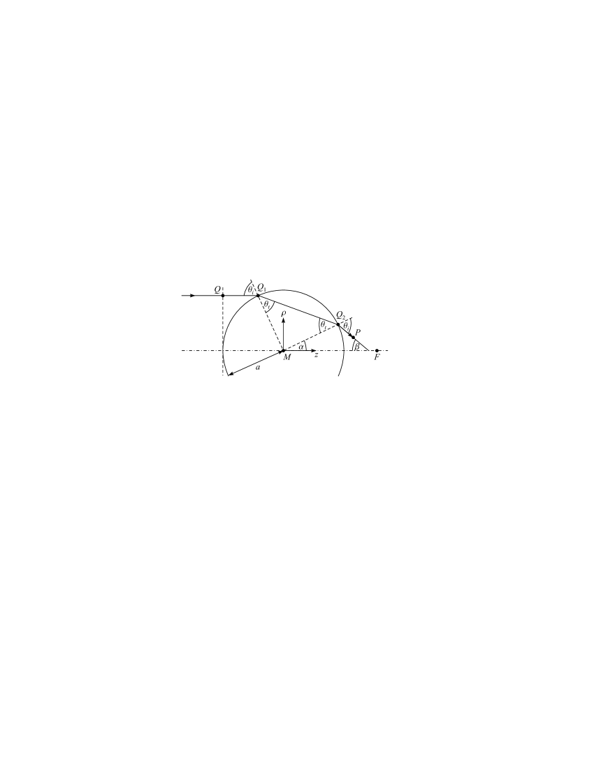
Figure 3: Refraction of a ray — propagating from $Q$ to $P$ — by a sphere with radius $a$ and refractive index $n$. The picture is drawn in the meridional plane and all indicated angles are positive.

Let $a$ be the sphere radius and $n>1$ its refractive index. In contrast to the previous sections, we choose the origin of the axially symmetric cylindrical coordinate system $(\rho,z)$ differently now, namely as the center $M$ of the sphere. The incident plane wave propagates parallel to the $z$-axis. The geometrical optics focus, formed by the paraxial rays, is located at $F\equiv(0,f)$ with Ber1978

$$f\equiv\dfrac{a}{2}\,\dfrac{n}{n-1}\,.$$ (43)

A ray passes the point $Q$, is first refracted at $Q_{1}$, a second time at $Q_{2}$ and propagates to $P$. The incident and transmitted angle, $\theta_{i}$ and $\theta_{t}$, are related by Snell’s law, $\sin\theta_{i}=n\sin\theta_{t}$. Writing the position of $P\equiv(\rho,z)$ in polar coordinates, $\rho=l\sin\theta$ and $z=l\cos\theta$, one can find the following expression, determining the three rays that arrive at $P$:

$$l\sin(\theta+2\,\theta_{i}-2\,\theta_{t})=a\sin\theta_{i}\,,$$ (44)

where one has to substitute $\theta_{t}=\arcsin[(\sin\theta_{i})/n]$. This is a transcendental cubic-like equation which has three roots, either all real or one real and two complex conjugate. (For $n\geq\sqrt{2}$ this is true for $z\geq a$; if $n<\sqrt{2}$, the 3-ray region does not start until some distance behind the sphere.) We denote them as $\theta_{i,j}(j=1,2,3)$ and choose their order consistently with the previous notations. Therefore, $\theta_{i,1}$ is always real and negative, whereas $\theta_{i,2}$ and $\theta_{i,3}$ are either real and positive (lit region) with $\theta_{i,2}<\theta_{i,3}$ or complex conjugate (geometrical shadow).

When the $\theta_{i,j}$ are known, we find the $\theta_{t,j}$ from Snell’s law and the $\alpha_{j}$ and $\beta_{j}$ from

$$\alpha=2\,\theta_{t}-\theta_{i}\,,\quad\beta=2\,\theta_{i}-2\,\theta_{t}\,.$$ (45)

Omitting the index $j$, the three ray coordinates can be written as

$$s\equiv\overline{Q_{2}P}=\dfrac{l\cos\theta-a\cos\alpha}{\cos\beta}\,.$$ (46)

The eikonal is the optical path accumulated from $Q$ to $P$ (on the dashed vertical line in figure 3 all rays are still in phase):

$$\psi =\overline{QQ_{1}}+n\,\overline{Q_{1}Q_{2}}+\overline{Q_{2}P}-a$$

$$=a\,(2\,n\cos\theta_{t}-\cos\theta_{i})+s\,.$$ (47)

The sphere radius $a$ was subtracted from the path contributions to make the eikonal zero in the center $M$, if there were no sphere.

Next we calculate the geometrical optics amplitudes by determining the meridional and sagittal radii of curvature, $R_{m}$ and $R_{s}$, and their changes due to refraction. Formulas for the refraction on an arbitrary surface with arbitrary orientation of the main radii exist in the literature.Kra1990 ; Cer2001 A simple derivation for the sphere can be found in appendix F. It yields the dependence of the actual radii of curvature $R_{m}$ and $R_{s}$ (right after the refraction) on the initial radii $R_{m0}$ and $R_{s0}$ (just before the refraction):

$$R_{m} =\dfrac{n\,a\,R_{m0}\cos^{2}\theta_{t}}{a\cos^{2}\theta_{i}+R_{m0}\,(\cos\theta_{i}-n\cos\theta_{t})}\,,$$ (48)

$$R_{s} =\dfrac{n\,a\,R_{s0}}{a+R_{s0}\,(\cos\theta_{i}-n\cos\theta_{t})}\,.$$ (49)

For a plane wave, $R_{m0},R_{s0}\rightarrow\infty$, the radii of curvature in the points $Q_{1}$ (inside the sphere) and $Q_{2}$ (outside the sphere) have the compact form

$$R_{m,Q_{1}} =-a\,\dfrac{\sin\theta_{i}\cos^{2}\theta_{t}}{\sin(\theta_{i}-\theta_{t})}\,,$$ (50)

$$R_{m,Q_{2}} =-a\,\dfrac{\cos\theta_{i}}{2}\left(\dfrac{\cos\theta_{i}\sin\theta_{t}}{\sin(\theta_{i}-\theta_{t})}-1\right)\!,$$ (51)

$$R_{s,Q_{1}} =-a\,\dfrac{\sin\theta_{i}}{\sin(\theta_{i}-\theta_{t})}\,,$$ (52)

$$R_{s,Q_{2}} =-a\,\dfrac{\sin(2\,\theta_{t}-\theta_{i})}{\sin(2\,\theta_{i}-2\,\theta_{t})}\,.$$ (53)

The overall geometrical generalized divergence after both refractions reads (index $j$ omitted)

$$\dfrac{1}{\sqrt{J}} =\dfrac{\sqrt{R_{m,Q_{1}}\,R_{s,Q_{1}}}}{\sqrt{(R_{m,Q_{1}}+d)\,(R_{s,Q_{1}}+d)}}$$

$$\quad\quad\quad\times\dfrac{\sqrt{R_{m,Q_{2}}\,R_{s,Q_{2}}}}{\sqrt{(R_{m,Q_{2}}+s)\,(R_{s,Q_{2}}+s)}}\,,$$ (54)

where $d\equiv 2\,a\cos\theta_{t}$ is the distance of propagation within the sphere. Note that ray 1 has a negative angle $\theta_{i}$. Besides, a double caustic phase shift should be added (manually) to the phase of this ray (minus sign) as in (18). The caustic shifts of the rays 2 and 3 are taken into account automatically if the branch cut for the square roots in (54) is along the negative real axis from $-\infty$ to $0$ and the branch with $\sqrt{-1}=+$i is used. In this procedure it is not allowed to multiply the radicands and write them under one common square root. Also the case of complex rays 2 and 3 is covered correctly by this convention.

Finally, the geometrical optics solution for the sphere is given by (20), where the eikonal $\psi$ and divergence $J$ are given by (47) and (54). The equation determining the three rays is (44). In the geometrical shadow the sum (20) becomes only the term with $j=1$.

To incorporate Fresnel transmission coefficients, we assume that the incident light is linearly polarized in $x$-direction, i.e., the incident electric field vector is

$$\mathbf{E}_{0}=E_{0}\,\mathbf{e}_{x}\,,$$ (55)

with $\mathbf{e}_{x}$ the unit vector in $x$-direction and $E_{0}\equiv U_{0}$. Since axial symmetry is broken, we introduce the polar angle $\varphi$ which is measured from $x$ to $y$. The point of observation $P\equiv(\rho,\varphi,z)$ will be reached by three rays (two may be complex) and their angles $\theta_{i,j}$ are still determined by (44), for all three rays lie in the meridional plane, containing $P$ and the $z$-axis (figure 4a). The initial $\pi$- and $\sigma$-polarized components depend on $\varphi$ (figure 4b):

$$E_{0,\pi} =E_{0}\cos\varphi\,,$$ (56)

$$E_{0,\sigma} =E_{0}\sin\varphi\,.$$ (57)

We define the overall transmission coefficients

$$T_{\pi} \equiv t_{12,\pi}\,t_{21,\pi}=1-r_{12,\pi}^{2}\,,$$ (58)

$$T_{\sigma} \equiv t_{12,\sigma}\,t_{21,\sigma}=1-r_{12,\sigma}^{2}\,.$$ (59)

Here the $t_{12}$ ($r_{12}$) are the standard Fresnel transmission (reflection) coefficients Bor2002 from the medium 1, i.e., vacuum, into the medium 2, i.e., the sphere.

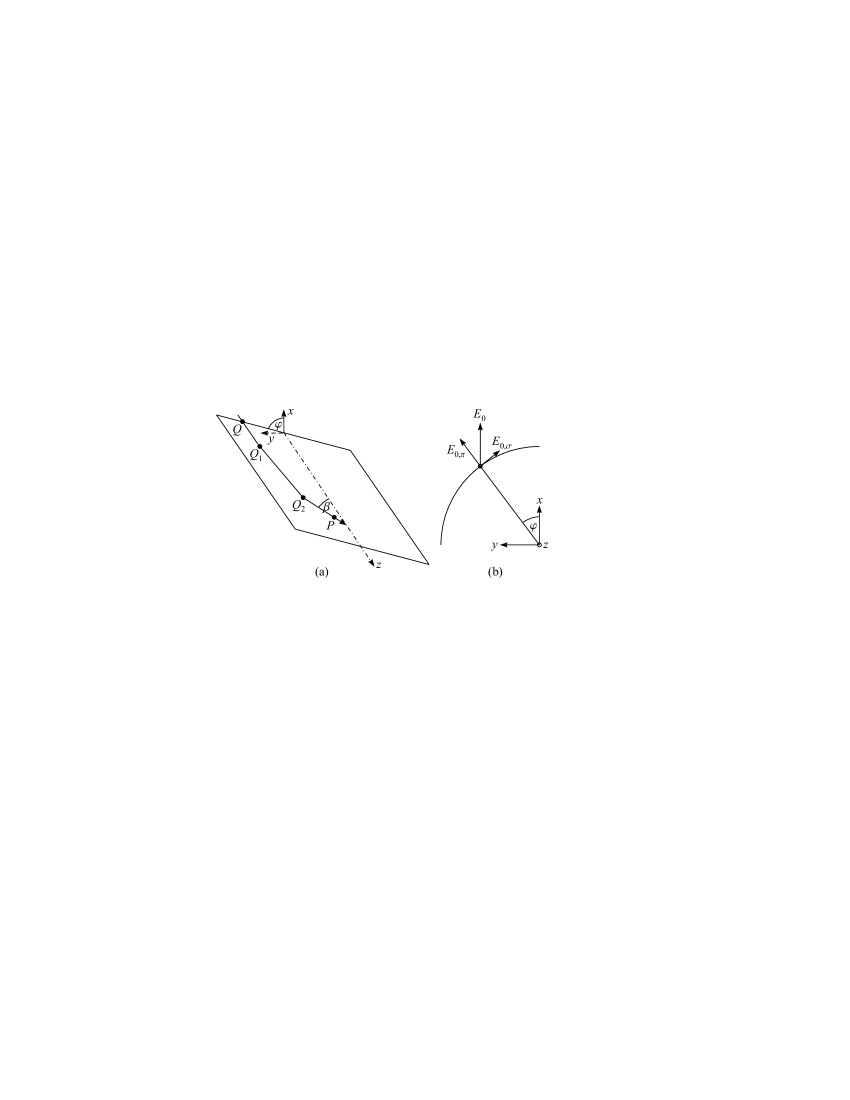
Figure 4: (a) A ray propagates from $Q$ to $P$ in the meridional plane (plane of incidence). (b) Decomposition of the initial electric field vector with length $E_{0}$ into its $\pi$- and $\sigma$-component parallel and perpendicular to the meridional plane

The ray field behind the sphere is found by the projection onto the original Cartesian system $(x,y,z)$. We write the components of the transmission vector $\mathbf{T}\equiv(T_{x},T_{y},T_{z})$ and show the ray index $j=1,2,3$ explicitly. The $\varphi$-dependence is indicated with the superscript $(m)$:

$$\begin{array}[c]{lll}T_{x,j}=T_{j}^{(0)}+T_{j}^{(2)}\cos 2\,\varphi\,,&&T_{j}^{(0)}\equiv\dfrac{T_{\pi,j}\cos\beta_{j}+T_{\sigma,j}}{2}\,,\vskip 3.0pt plus 1.0pt minus 1.0pt\\ T_{y,j}=T_{j}^{(2)}\sin 2\,\varphi\,,&&T_{j}^{(1)}\equiv T_{\pi,j}\sin\beta_{j}\,,\vskip 3.0pt plus 1.0pt minus 1.0pt\\ T_{z,j}=T_{j}^{(1)}\cos\varphi\,,&&T_{j}^{(2)}\equiv\dfrac{T_{\pi,j}\cos\beta_{j}-T_{\sigma,j}}{2}\,.\end{array}$$ (60)

Hence, the geometrical optics solution for the electric field $\mathbf{E}\equiv(E_{x},E_{y},E_{z})$ — including the eikonal $\psi$ (47) and divergence $J$ (54) — reads

$$\begin{array}[c]{lll}E_{x,j}=E_{j}^{(0)}+E_{j}^{(2)}\cos 2\,\varphi\,,&&\\ E_{y,j}=E_{j}^{(2)}\sin 2\,\varphi\,,&&E_{j}^{(m)}\equiv E_{0}\,\dfrac{T_{j}^{(m)}\,\text{e}^{\,\text{i}\,k\,\psi_{j}}}{\sqrt{J_{j}}}\,.\\ E_{z,j}=E_{j}^{(1)}\cos\varphi\,,&&\end{array}$$ (61)

IV.2 The Bessoid matching solution

Matching each term $E^{(m)}=\sum\nolimits_{j=1}^{3}E_{j}^{(m)}$ by the Ansatz (21) in its higher-order formulation (40) with the corresponding integral $I_{m}$, we obtain the vectorial electric field $\mathbf{E}\equiv(E_{x},E_{y},E_{z})$ in the form

$$\mathbf{E}=E^{(0)}\!\left(\begin{array}[c]{c}1\\ 0\\ 0\end{array}\right)+E^{(1)}\!\left(\begin{array}[c]{c}0\\ 0\\ \cos\varphi\end{array}\right)+E^{(2)}\!\left(\begin{array}[c]{c}\cos 2\,\varphi\\ \sin 2\,\varphi\\ 0\end{array}\right)\!.$$ (62)

Figure 5 illustrates the intensity, i.e., the absolute square of the electric field $\left|E\right|^{2}\equiv\mathbf{E}\,\mathbf{E}^{\ast}$, for $\varphi=0$ ($x$,$z$-plane) and $\varphi=\pi/2$ ($y$,$z$-plane).

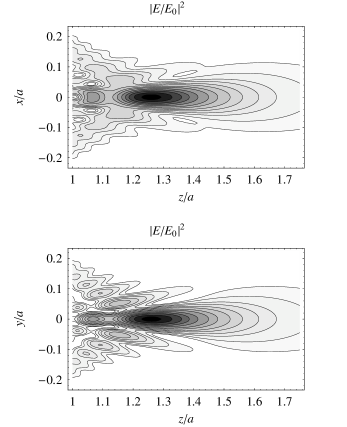
Figure 5: Normalized intensity $\left|E/E_{0}\right|^{2}$ in the normalized $x$,$z$-plane (top) and in the $y$,$z$-plane (bottom). Contour shadings go from white (zero) to black ($\approx 700$). Parameters: refractive index $n=1.5$, dimensionless wavenumber $k\,a=100$. The initial electric field vector is $\mathbf{E}_{0}=E_{0}\,\mathbf{e}_{x}$. The sphere with radius $a$ is situated in the origin. The focus of geometrical optics is located at $z=f=1.5\,a$, whereas the diffraction focus (the point of maximum intensity) is significantly shifted towards the sphere: $f_{d}\approx 1.25\,a$. In dimensional units, for a wavelength of $\lambda=0.248\,$$\mu$m the sphere radius is $a\approx 4\,$$\mu$m.

The magnetic field $\mathbf{H}$ can be calculated similarly (incident magnetic field $\mathbf{H}_{0}=H_{0}\,\mathbf{e}_{y}$, $H_{0}=E_{0}$) and the (normalized) Poynting vector is given by $\mathbf{S\equiv}\operatorname{Re}(\mathbf{E\!}\times\mathbf{\!H}^{\ast})$.

IV.3 On the axis

On the axis the electric field is given by its $x$-component only (direction of polarization) due to averaging over $\varphi$ in (62). For $z<f$ (inside the cusp) it is given by the analytical expression (37). After several simplifications Kof2004 it can be written as

$$E=E_{0}\left[\,T_{1}\,D_{1}\!\left(\text{i}\,I-\dfrac{1}{Z}\right)+\dfrac{T_{2}}{1-z/f}\,\right]\text{e}^{\,\text{i}\,\varphi_{2}}\,,$$ (63)

where the transmission factors $T_{j}\equiv T_{j}^{(0)}$ are given in (60) and for dielectric spheres have the form:

$$T_{1} =\dfrac{n\,(1+3\cos\beta_{1})\cos\theta_{i,1}\cos\theta_{t,1}}{(n\cos\theta_{i,1}+\cos\theta_{t,1})^{2}}\,,$$ (64)

$$T_{2} =\dfrac{4\,n}{1+n^{2}}\,.$$ (65)

The phases in the coordinate $Z=-2\,\sqrt{\varphi_{1}-\varphi_{2}}$ are

$$\varphi_{1} =\varphi_{3}=k\,a\left(2\,n\cos\theta_{t,1}-\cos\theta_{i,1}+\dfrac{\sin\alpha_{1}}{\sin\beta_{1}}\right)\!,$$ (66)

$$\varphi_{2} =2\,k\,a\,(n-1)+k\,z\,,$$ (67)

and $D_{1}\equiv\sqrt{\varphi_{1}-\varphi_{3}}/\sqrt{J_{1}}$ is the first ray’s compensated sagittal divergence:

$$D_{1} =-\dfrac{\sqrt{(R_{m,Q_{1}})_{1}\,(R_{s,Q_{1}})_{1}}}{\sqrt{[(R_{m,Q_{1}})_{1}+d_{1}]\,[(R_{s,Q_{1}})_{1}+d_{1}]}}$$

$$\quad\quad\quad\times\dfrac{\sqrt{(R_{m,Q_{2}})_{1}\,(R_{s,Q_{2}})_{1}}}{\sqrt{(R_{m,Q_{2}})_{1}+s_{1}}}\,\sqrt{2\,k}\,\sin\beta$$

$$=-2\,\sqrt{2\,k\,a}\,\cos(\beta_{1}/2)$$

$$\quad\quad\quad\times\sqrt{\dfrac{\cot\theta_{i,1}\cos\theta_{t,1}\sin(\beta_{1}/2)}{1+1/n^{2}-3\sin^{2}(\beta_{1}/2)/\sin^{2}\theta_{i,1}}}\,,$$ (68)

which manifestly has no singularity until the geometrical focus where $(R_{m,Q_{2}})_{1}+s_{1}\rightarrow 0$. The minus sign comes from the manually inserted phase shift of the first ray. (All aforementioned quantities should be expressed in terms of the angles $\theta_{i,1}$ and $\theta_{i,2}\equiv 0$ as described in detail in section IV.4 below.) The structure of the first two lines in (68) is general and is valid for arbitrary axially symmetric systems. $D_{1}$ is always finite on the axis, since both the sagittal radius of curvature and the phase difference $\varphi_{1}-\varphi_{3}$ are proportional to the distance $\rho$.

Equation (63) is valid even near the focus, since the diverging terms $D_{1}/Z$ and $(1-z/f)^{-1}$ almost cancel. For $z\rightarrow f$, however, the divergence of $D_{1}$ itself becomes important, as the non-paraxial ray 1 becomes axial.

In figure 6 we show the position and the value of the maximum of $\left|E\right|^{2}$ as a function of the refractive index and the dimensionless product $k\,a$, calculated from (63). The $z$-coordinate of this global maximum is denoted with $f_{d}$ (diffraction focus) and the intensity there is $\left|E(f_{d})\right|^{2}$. Contrary to the square dependence for the case of an ideal lens,Bor2002 even for macroscopic spheres the maximum intensity turns out to be about proportional to $k\,a$, in agreement with the general theory.Kra1999

Figure 6: Left: Diffraction focus in units of the sphere radius as a function of $n$ and $k\,a$ (contour lines from top to bottom go from 1.1 to 3.0 in steps of 0.1). Right: Intensity enhancement at $f_{d}$ (contour lines from bottom left to top right are 20, 50, 100, 200, 500, 1000 and 2000)

The main contribution in (63) stems from the Bessoid integral, that is from the term $\propto T_{1}\,D_{1}\,I$. Thus, the position of the maximum can be estimated from condition (35), i.e., $\varphi_{1}-\varphi_{2}\approx 3\,\pi/4$. If the phase difference $\varphi_{1}-\varphi_{2}$ from (66) and (67) is expressed as a function of $\theta_{i,1}$, Taylor expanded and equated to $3\,\pi/4$, then we get in the lowest non-trivial order of the inverse product $k\,a$:

$$f_{d}\approx\dfrac{a}{2}\,\dfrac{n}{n-1}\left(1-\sqrt{\dfrac{3\,\pi}{4\,k\,a}\,\dfrac{n\,(3-n)-1}{n\,(n-1)}}\,\right)\!.$$ (69)

Hence, in the limit of small wavelengths or large spheres the relative difference between the diffraction and the geometrical focus decreases proportionally to the inverse square root of $k\,a$. The factor $3\,\pi/4\approx 2.356$ can be replaced by the more exact Bessoid value 2.327 from (35). Expression (69) approximates the position of the maximum within an error of $<5\,\%$ for $k\,a>100$ and values of the refractive index in the range $1.4<n<1.6$. The transcendental phase difference condition (35), which holds for large angles, naturally has a wider range of applicability. With very good accuracy the diffraction focus also provides the maximum for the absolute square of the magnetic field, $\left|H\right|^{2}\equiv\mathbf{H}\,\mathbf{H}^{\ast}$, as well as for the $z$-component of the Poynting vector $\mathbf{S}$. Note that on the axis $\mathbf{H}=H\,\mathbf{e}_{y}$ and $\mathbf{S}=S\,\mathbf{e}_{z}$.

IV.4 A protocol for the electromagnetic field calculation behind the sphere

For convenience we summarize the sequence of steps that should be used for the calculation of the field behind a sphere irradiated with linearly polarized light on the basis of the formulas developed above:

1. Finding the rays: The origin of the coordinate system is in the center of the sphere. Choose a point $P\equiv(\rho,\varphi,z)$ behind the sphere and numerically calculate the 3 rays arriving at $P$. These rays are characterized by the 3 incident angles $\theta_{i,j}$ ($j=1,2,3$), found numerically from (44), and numbered according to figure 2. All other angles follow from Snell’s law and from (45), respectively. Outside the cuspoid the rays 2 and 3 are complex.

2. The geometrical optics solution: Compute the geometrical optics solution for the electric field (61), which is the sum of contributions from three rays. The eikonals $\psi_{j}$ are calculated from (47) with (46). The geometrical optics amplitudes are given by the Fresnel transmission components $T_{j}^{(m)}$ (60) and the generalized divergence factors $1/\sqrt{J_{j}}$ (54), which follow from the radii of curvature (50)–(53) and the distances $s_{j}$ from the sphere to $P$ (46). The conventions for the complex roots shall correctly add up all individual caustic phase shifts. Ignore the fact that the geometrical field diverges near caustic regions.

3. Bessoid matching: Starting from the eikonals $\psi_{j}$, determine the Bessoid coordinates, i.e., first $Z$, and then $R$ and $\chi$ (28). Next, compute and correctly order the points of stationary phase $t_{j}$ (26), most conveniently using trigonometric formulas.Bro2004 With the generalized divergences (54) and the Hessians (25) the Bessoid amplitudes $A_{m}$, $A_{mR}$ and $A_{mZ}$ can be computed from (42) for all orders $m=0,1,2$. The electric field component $E^{(m)}$ associated with the $m$-th order results from the Ansatz (40). The Bessoid-matched field $\mathbf{E}$ is finally given by (62). In the case of a scalar plane wave (or exactly on the axis) only the order $m=0$ contributes. Proceed accordingly for the magnetic field $\mathbf{H}$, employing different transmission coefficients in step 2.

4. The Bessoid integral: The final solution (62) contains the Bessoid integral and higher-order Bessoid integrals as well as their partial derivatives. The Bessoid integral $I(R,Z)$ can be efficiently computed numerically via the differential equation (12). The higher-order Bessoid integrals follow from a recursive relation (39).

5. Remarks: The speed limiting bottleneck of this procedure is the finding of the rays $\theta_{i,j}$ in step 1. The numerical evaluation of the Bessoid integral is very efficient and in all other steps analytical expressions are applied. When approaching the caustic (axis, cuspoid), individual quantities — the geometrical optics amplitudes — diverge but their combinations remain finite. In our calculations we observed perfect numerical stability up to distances from the caustic of the order of $10^{-5}$ times the sphere radius, which is more than enough for any practical purposes.

IV.5 Comparison with the theory of Mie

We presented a general way to match geometrical optics solutions with the Bessoid integrals. It can be applied to any axially symmetric system with the cuspoid topology of spherical aberration.

For the sphere we can compare our approximate results with the theory of Mie.Mie1908 A main quantity characterizing the sphere is the dimensionless Mie parameter $q\equiv k\,a$. Figure 7 compares the intensity on the axis obtained from the Mie theory with the Bessoid approximation. The parameters are as in figure 5 and the Mie parameter is $q=300$, $100$, $30$ and $10$.

Figure 7: $\left|E/E_{0}\right|^{2}$ on the axis. Dashed lines represent the Mie theory, solid lines are the results of Bessoid matching. The parameters are as in figure 5 and the cases (a), (b), (c) and (d) correspond to $q=300$, $100$, $30$ and $10$, respectively. In dimensional units, for $\lambda=0.248\,$$\mu$m this corresponds to sphere radii of $a\approx 12\,$$\mu$m, $4\,$$\mu$m, $1.2\,\mu$m and $0.4\,\mu$m.

We see very good agreement down to $q\approx 30$ ($a/\lambda\approx 4.8$). For $q=10$ ($a/\lambda\approx 1.6$) the asymptotic behavior far from the sphere is still correct. However, for small $q$ the characteristic scale $a$ is no longer large compared to the wavelength $\lambda$ and geometrical optics becomes invalid.

Next, we compare the off-axis electric and magnetic field as well as the $z$-component of the Poynting vector, $S_{z}$ (figure 8). Right behind the sphere ($z=a$) the agreement is not perfect (see figure 7), though all qualitative features are preserved. Sections at $z=1.02\,a$ already show good agreement (figure 8) and for $z\gtrsim 1.05\,a$ the pictures become visually almost indistinguishable. Discussing the quality of these results, one has to differentiate between the accuracy of the method and the influence of those factors which can be taken into account, but were not included into the current consideration.

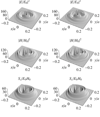
Figure 8: Normalized $\left|E\right|^{2}$, $\left|H\right|^{2}$ and $S_{z}$ in the normalized $x$,$y$-plane for $z=1.02\,a$ calculated with Bessoid matching (left) and with the Mie theory (right). The parameters are the same as in figure 5.

The accuracy of the Bessoid matching procedure itself was studied separately for the case of a spherically aberrated wave incident onto an aperture. The deviation — defined as the maximal relative error of the intensity $(|E_{\text{Bessoid}}|^{2}\!-\!|E_{\text{exact}}|^{2})/|E_{\text{exact}}|^{2}$ — between the Bessoid matched geometrical optics solution and the corresponding (exact) Rayleigh–Sommerfeld diffraction integralBor2002 decreases as the aperture increases. If the aperture is large enough, the deviation is below $10^{-3}$ for spherical abberation strengths and wavevectors approximately corresponding to the focusing by spheres studied in figures 7 and 8.

For the sphere, for all investigated Mie parameters $30\leq q\leq 300$, the deviations from the exact Mie solution are about $\pm 5\,\%$ in those regions where the intensity is not very small (including the caustic axis and cuspoid). A detailed analysis indicates that this deviation originates from several factors:

(i) Influence of the finite size of the sphere. There exist diffractive contributions from creeping raysKel1962 propagating along the sphere surface. They can in principle be accounted for at the expense of the simplicity of the procedure, essentially by considering the interference of the Bessoid field with these additional rays. This results in oscillations which can actually be seen in the Mie curve on the right side of the Bessoid tail in figures 7a and b.

(ii) Rays entering the sphere undergo multiple interior reflections. Some of them satisfy resonance conditions, accumulate significant energy inside the sphere and refract outside. This produces an additional field behind the sphere, in particular the intensity becomes non-zero in the regions of geometrical shadow for the directly transmitted rays used in the Bessoid matching. Here again, one can (in principle) study such multiply reflected rays separately and add them to the Bessoid field, but their contribution to the focusing properties of the microspheres is of secondary importance.

(iii) Finally, very close to the sphere surface at distances of the order of a fraction of $\lambda$, there exist evanescent contributions, which are taken into account in the Mie theory, but are obviously absent in the Bessoid matching procedure.

Thus, the quality of the Bessoid matching in the most interesting regions near caustic surfaces is quite satisfactory. It rectifies the divergences of geometrical optics, which is asymptotically correct for large $q$ in non-singular regions of space. Clearly, the procedure has to be extended whenever contributions from rays other than those 3 used for matching become significant.

The field distribution behind the sphere has a rich fine structure (figure 8) which our geometrical approach helps to clarify. It is known that the ring-type field enhancement corresponds to the cuspoid caustic, having the approximate radial distanceLuk2003

$$\rho_{\text{c}}=a\,\dfrac{(4-n^{2})^{3/2}}{3\,\sqrt{3}\,n^{2}}\,.$$ (70)

Our approach explains the double-peak structure of $\left|E\right|^{2}$ along the direction of polarization. It is related to the axial field component $E_{z}$ and can be understood in terms of geometrical optics. On the axis, the $E_{z}$ components from the rays 1 and 3 point into opposite directions and cancel, having an effective phase difference of $\pi$. Off the axis, ray 1 underwent a caustic phase shift of $-\pi/2$ when crossing the axis, which makes the condition for constructive interference: $\varphi_{1}-\varphi_{3}=3\,\pi/2$. Then, according to (34), the peak occurs at the radial distance

$$\rho_{\text{p}}\approx\dfrac{\varphi_{1}-\varphi_{3}}{2\,k\,\sin\beta}=\dfrac{3}{8}\,\dfrac{\lambda}{\sin\beta}\,.$$ (71)

More details on the derivation are given elsewhereKof2004 together with the refined coefficient 0.293 (instead of $3/8$) obtained from the Bessoid asymptotic (110).

Double-peak structures have been observed in nano-patterning experimentsMue2001 ; Bae2003 ; Lan2005 and were semi-quantitatively explained on the basis of the Mie solution.Luk2002 In an actual experiment it may depend on the laser pulse parameters and the properties of the patterned material, whether the Poynting vector or the electric field is responsible for the patterning process. For small spheres this double peak effect can be understood using the near field pattern for a scattering dipole.Luk2002 ; Luk2003 The present explanation (for sphere diameters of a few wavelengths and larger) results in the same orientation of the maxima and thus these two limiting cases cover almost all range of sphere sizes. Similar polarization dependence of the field distribution in focal regions can be used to improve the resolution.Dor2003

V Conclusions

We described theoretically arbitrary axially symmetric aberrated focusing and studied light focusing by microspheres as an example. Following the method of uniform caustic asymptotics,Kra1999 we introduced a canonical integral describing the wave field for the given cuspoid ray topology. This Bessoid integral appears naturally in the paraxial approximation. In some regions (off the caustic or exactly on the axis) it reduces to simple analytical expressions. In other regions we efficiently computed this highly oscillatory integral via a single ordinary differential equation.

For arbitrary axially symmetric focusing, coordinate and amplitude transformations match the Bessoid wave field and the solution of geometrical optics. The caustic divergences of the latter are removed thereby. For vectorial problems with angularly dependent field components, higher-order Bessoid integrals are used for the matching procedure. The formulas significantly simplify on and near the axis. An approximate universal condition for the diffraction focus can be given in terms of phase differences. Here, the concept of caustic phase shifts is of main importance.

The central part of the Bessoid integral is essentially a Bessel beamMcG2005 with a variable cross section due to the variable angle of the non-paraxial rays. Its local diameter is always smaller than in the focus of an ideal lens with the same numerical aperture. Besides, the largest possible apertures can be physically realized, which is hardly possible with lenses. All this is achieved at the expense of longitudinal confinement.

As an example the focusing of a linearly polarized plane wave by a transparent sphere is studied in detail. We calculate the geometrical optics eikonals and divergences, incorporate Fresnel transmission coefficients and perform Bessoid matching. Using the general theory, simple expressions for the light field on the axis and for the diffraction focus are derived. The two strong maxima in the intensity observed immediately behind the sphere can be explained as well.

Finally, the results of the Bessoid matching procedure are compared with the Mie theory. The agreement is good for Mie parameters $k\,a>30$. Near the sphere the correspondence is worse due to unaccounted evanescent contributions.

The developed formulas can be directly applied in other areas of physics where non-paraxial axially symmetric focusing is of importance, e.g., acoustics, semiclassical quantum mechanics,Pet1997 flat superlenses based on left-handed materials,Par2003 radio wave propagation, scattering theory,Con1981 chiral conical diffractionBer2006 etc.

Concluding, let us briefly enumerate several possibilities to extend and refine the developed formalism. Weak absorption can be incorporated easily, for it just changes the amplitudes along the rays and the transmission coefficients. Strong absorption additionally modifies Snell’s law of refraction, still preserving the axial symmetry. One can consider incoming radially or azimuthally polarized beams, which are known to produce better resolution than linear polarization.Dor2003 The diffraction of light from regions beyond the sphere radius can be incorporated by considering the interference of the Bessoid field with creeping rays.Kel1962 For other geometries, in particular finite apertures with sharp boundaries, edge rays or the Rubinowitz representation,Bor2002 or an approach based on catastrophe theoryNye2005 have to be used. Such corrections become relevant, for example, for the ray structure and the field distribution immediately behind spheres with a refractive index $n<\sqrt{2}$. Finally, one can calculate the interference of the diffracted light with the original incident wave or the interference of the light refracted by several spheres or arrays of spheres. The latter yields interesting secondary patterns Bae2002 related to the so called Talbot effect.Ber2001

Acknowledgments

The authors thank D. Bäuerle (Johannes Kepler University, Linz) for many stimulating discussions on microsphere patterning experiments, which initiated this study, and for his continuous support of this work. The authors also thank B. Luk’yanchuk and Z. B. Wang (both at the Data Storage Institute, Singapore) for their Mie program and discussions on Mie calculations. J. K. appreciates helpful conversations with G. Langer (Johannes Kepler University, Linz). N. A. thanks V. Palamodov (Tel Aviv University) for illuminating mathematical suggestions. Financial support was provided by the FWF (Austrian Science Fund) under Contract No. P16133–N08. N. A. also thanks the Christian Doppler Laboratory of Surface Optics (Johannes Kepler University, Linz).

Appendix A A near axis approximation for the Bessoid integral

We make the substitution $w\equiv\rho_{1}^{2}$ in (2):

$$I(R,Z)=\dfrac{1}{2}\,\int\nolimits_{0}^{\infty}J_{0}(R\sqrt{w})\;\text{e}^{-\,\text{i}\,\left(Z\,\tfrac{w}{2}\,+\,\tfrac{w^{2}}{4}\right)}\text{d}w\,.$$ (72)

Near the axis (small $R$) the Bessel function is slowly varying compared with the exponent. The integral will have significant contribution only from the region in which the exponent’s phase is stationary, i.e., regions near $w=-Z$. We consider the most interesting caustic part of the axis for which $Z\leq 0$. In a lowest order approximation the Bessel function is considered as constant near the stationary point $-Z$ and can be pulled out of the integral. The phase can be written as a complete quadratic form. With the full square of $v\equiv(w+Z)/2$:

$$I(R,Z)\approx J_{0}(R\sqrt{-Z})\;\text{e}^{\,\text{i}\,\tfrac{Z^{2}}{4}}\int\nolimits_{Z/2}^{\infty}\text{e}^{-\,\text{i}\,v^{2}}\text{d}v\,.$$ (73)

The remaining integral can be expressed in terms of the complementary error functionAbr1993 erfc (of complex argument) and hence we arrive at (11).

For $Z>0$ the point $w=0$ should be taken as a stationary edge point of the integration.Foc1956 And the near axis approximation (11) remains valid as long as the Bessel function is set to $J_{0}(0)=1$.

Appendix B An ordinary differential equation for the Bessoid integral

We derive the paraxial Helmholtz equation

$$I_{RR}+\dfrac{1}{R}\,I_{R}+2\,\text{i}\,I_{Z}=0\,,$$ (74)

as well as the following ordinary differential equation for the Bessoid integral:

$$I_{RRR}+\dfrac{1}{R}\,I_{RR}-\left(\dfrac{1}{R^{2}}+Z\right)I_{R}+\text{i}\,R\,I=0\,.$$ (75)

Indices denote partial derivatives. Both equations can be rewritten in the compact form

$$L+2\,\text{i}\,I_{Z} =0\,,$$ (76)

$$L_{R}-Z\,I_{R}+\text{i}\,R\,I =0\,,$$ (77)

where $L$ is the radial Laplacian

$$L\equiv I_{RR}+\dfrac{1}{R}\,I_{R}\,.$$ (78)

We begin with the proof of (74) and state that we may differentiate under the integral sign, since the partial derivatives of the integrand exist and are continuous functions. Starting from the Bessoid integral in the polar representation (2), its integrand can be written as

$$G\equiv\rho_{1}\,J_{0}(R\,\rho_{1})\,E\,,$$ (79)

with the abbreviation

$$E\equiv\text{e}^{-\,\text{i}\,\left(Z\,\tfrac{\rho_{1}^{2}}{2}\,+\,\tfrac{\rho_{1}^{4}}{4}\right)}.$$ (80)

The (multiple) partial derivatives are

$$G_{R} =-\rho_{1}^{2}\,J_{1}(R\,\rho_{1})\,E\,,$$ (81)

$$G_{RR} =-\dfrac{\rho_{1}^{3}}{2}\,[J_{0}(R\,\rho_{1})-J_{2}(R\,\rho_{1})]\,E\,,$$ (82)

$$G_{Z} =-\text{i}\,\dfrac{\rho_{1}^{3}}{2}\,J_{0}(R\,\rho_{1})\,E\,.$$ (83)

Here we used the derivative formula for Bessel functionsAbr1993

$$\dfrac{\text{d}}{\text{d}t}\,J_{m}(t)=\dfrac{J_{m-1}(t)-J_{m+1}(t)}{2}$$ (84)

with $m=0$ to obtain (81) and $m=1$ for (82). Note that $J_{-1}(t)=-J_{1}(t)$. Applying the recurrence relation for Bessel functionsAbr1993

$$J_{m+1}(t)=-J_{m-1}(t)+\dfrac{2\,m}{t}\,J_{m}(t)\,,$$ (85)

one can eliminate $J_{2}$ from (82). And then it is enough to notice and verify that

$$G_{RR}+\dfrac{1}{R}\,G_{R}+2\,\text{i}\,G_{Z}=0\,.$$ (86)

This proves equation (74).

For the proof of (75), we need to note that its left hand side can be expressed as the integral of a partial derivative

$$H\equiv{\displaystyle\int\nolimits_{0}^{\infty}}\dfrac{\partial}{\partial\rho_{1}}\!\left[\,\text{i}\,\rho_{1}\,J_{1}(R\,\rho_{1})\;\text{e}^{-\,\text{i}\,\left(Z\,\tfrac{\rho_{1}^{2}}{2}\,+\,\tfrac{\rho_{1}^{4}}{4}\right)}\right]\!\text{d}\rho_{1}.$$ (87)

With the help of (84) and (85) both the left hand side of (75) and $H$ become

$${\displaystyle\int\nolimits_{0}^{\infty}}[\,\text{i}\,R\,\rho_{1}\,J_{0}(R\,\rho_{1})+\rho_{1}^{2}\,(Z+\rho_{1}^{2})\,J_{1}(R\,\rho_{1})]\,E\,\text{d}\rho_{1}.$$ (88)

Thus, in order to prove (75), it is enough to show that $H=0$. This follows from the Newton-Leibniz formula applied to the (definite) integral (87):

$$H=\left[\,\text{i}\,\rho_{1}\,J_{1}(R\,\rho_{1})\;\text{e}^{-\,\text{i}\,\left(Z\,\tfrac{\rho_{1}^{2}}{2}\,+\,\tfrac{\rho_{1}^{4}}{4}\right)}\right]_{0}^{\infty}=0\,.$$ (89)

The lower bound at $0$ vanishes for obvious reasons. For the upper bound at $\infty$ one assumes an infinitely small imaginary part in front of the fourth order term in the exponent: $\rho_{1}^{4}\rightarrow(1-\,$i$\,\varepsilon)\,\rho_{1}^{4}$ with $\varepsilon>0$. This completes the proof of the differential equations (74) and (75) for the Bessoid integral.

Appendix C The near axis Bessoid coordinates

Near the axis the phases of the rays can be Taylor expanded. From figure 9 one infers that up to the first order in $\rho$ the phases can be written as

$$\varphi_{1} \approx\varphi_{\text{np}}+k\,\rho\,\sin\beta\,,$$

$$\varphi_{2} \approx\varphi_{\text{p}}\,,$$ (90)

$$\varphi_{3} \approx\varphi_{\text{np}}-k\,\rho\,\sin\beta\,.$$

Here $\varphi_{\text{np}}$ and $\varphi_{\text{p}}$ denote the phases of the non-paraxial rays and the (par)axial ray (with $\rho=0$) and $\beta>0$ is the angle of ray 3 with the axis.

Figure 9: Near the axis, the phases of the rays 1 and 3 differ from the phase of the non-paraxial rays np (crossing the axis at the same $z$) by $\pm\,k\,\rho\,\sin\beta$, whereas the phases of ray 2 and the (par)axial ray are the same in first order. The non-paraxial ray and ray 3 cross the axis at an angle $\beta>0$.

We insert these phases into the exact expressions for $R$ and $Z$ in (28), Taylor expand the result with respect to $\rho$ and resubstitute $\varphi_{\text{np}}\approx(\varphi_{1}+\varphi_{3})/2$, $\varphi_{\text{p}}\approx\varphi_{2}$ and $k\,\rho\,\sin\beta\approx(\varphi_{1}-\varphi_{3})/2$ from (90). This yields (32) and (33).

Appendix D The on axis field

Here we derive a simple on axis expression for the Bessoid-matched field $U$ (21), namely equation (37).

On the axis and inside the cusp $\rho=0$ ($R=0$) and $z<0$ ($Z<0$). The stationary points, given by (26), are

$$t_{1}=-\sqrt{-Z}\,,\quad t_{2}=0\,,\quad t_{3}=-t_{1}\,.$$ (91)

Then, the amplitude $A$ in (31) simplifies to

$$A=U_{0,2}\,\dfrac{\sqrt{H_{2}}}{\sqrt{J_{2}}}\,,$$ (92)

because on the axis the ratios $\sqrt{H_{1,3}}/\sqrt{J_{1,3}}$ are both finite and the corresponding other terms disappear upon multiplication with $t_{2}=0$. Due to the restriction to the lit region ($Z<0$), all rays are real and equation (24) holds. By virtue of (9) $\det\mathbf{H}_{2}=Z^{2}$, and due to (10) sign$\,\mathbf{H}_{2}=2$, one finds

$$\sqrt{H_{2}}=\text{i}\,Z\,,$$ (93)

and thus:

$$A=\text{i}\,\dfrac{U_{0,2}\,Z}{\sqrt{J_{2}}}\,.$$ (94)

This approximation for the amplitude $A$ is valid up to the focus ($Z=0$). As ray 2 converges like the inverse distance from the focus, $\sqrt{J_{2}}$ is proportional to $Z$.

The amplitude $A_{R}$ in (31) vanishes due to $t_{3}=-t_{1}$ and the fact that

$$\dfrac{\sqrt{H_{1}}}{\sqrt{J_{1}}}=\dfrac{\sqrt{H_{3}}}{\sqrt{J_{3}}}\,,$$ (95)

which means that rays 1 and 3 have equal amplitudes and that the caustic phase shifts are in accordance with the signature of the Hessian. Consequently,

$$A_{R}=0\,.$$ (96)

With (91) and (95) the amplitude $A_{Z}$ reads

$$A_{Z}=\dfrac{2}{Z}\left(U_{0,1}\,\dfrac{\sqrt{H_{1}}}{\sqrt{J_{1}}}-U_{0,2}\,\dfrac{\sqrt{H_{2}}}{\sqrt{J_{2}}}\right)\!.$$ (97)

The first term is non-trivial. Both $\sqrt{H_{1}}$ and $\sqrt{J_{1}}$ are zero on the axis, but their ratio is finite and well defined. Indeed, the Taylor expansion of Cardan’s solution $t_{1}$ in its trigonometric representationBro2004 yields in the first order in $R$:

$$t_{1}=-\sqrt{-Z}+\dfrac{R}{2\,Z}\,.$$ (98)

Therefore, again in first order in $R$: $\det\mathbf{H}_{1}=2\,R\,\sqrt{-Z}$. Due to sign$\,\mathbf{H}_{1}=-2$ we obtain

$$\sqrt{H_{1}}=\text{i}\,\sqrt{2\,R\,\sqrt{-Z}}\,,$$ (99)

and with (93):

$$A_{Z}=2\,\text{i}\,\dfrac{U_{0,1}\sqrt{2\,R\,\sqrt{-Z}}}{Z\,\sqrt{J_{1}}}-2\,\text{i}\,\dfrac{U_{0,2}}{\sqrt{J_{2}}}\,.$$ (100)

This approximation for $A_{Z}$ holds for small values of $R$. It is finite, since $\sqrt{J_{1}}$ approaches zero as $\sqrt{R}$ for $R\rightarrow 0$.

For the final representation of the field $U$, we can substitute the near axis expression for $R\sqrt{-Z}$ (34) into $A_{Z}$. On the axis the phase coordinate becomes $\chi=\varphi_{2}$, which results from substituting $\varphi_{1}=\varphi_{3}$ and $Z=-2\,\sqrt{\varphi_{1}-\varphi_{2}}$ into the corresponding expression in (28). This leads to

$$U =\left(A\,I+\dfrac{1}{\text{i}}\,A_{R}\,I_{R}+\dfrac{1}{\text{i}}\,A_{Z}\,I_{Z}\right)\text{e}^{\,\text{i}\,\chi}$$ (101)

$$=\left(\dfrac{U_{0,2}}{\sqrt{J_{2}}}\,(\text{i}\,Z\,I-2\,I_{Z})+\dfrac{2\,U_{0,1}\,\sqrt{2\,k\,\rho\,\sin\beta}}{Z\,\sqrt{J_{1}}}\,I_{Z}\right)\text{e}^{\,\text{i}\,\varphi_{2}}.$$

Using the linear relationship between the Bessoid integral and its $Z$-derivative (15),

$$\text{i}\,Z\,I-2\,I_{Z}=1\,,$$ (102)

we end up with equation (37).

Appendix E Higher-order Bessoid integrals

Higher-order Bessoid integrals (38) appear naturally, if one expands an arbitrary initial field amplitude on the aperture in a Fourier series:

$$U_{0}(\rho_{1},\varphi_{1})={\displaystyle\sum\limits_{m=0}^{\infty}}\,[\,a_{m}(\rho_{1})\cos(m\,\varphi_{1})+b_{m}(\rho_{1})\sin(m\,\varphi_{1})\,]\,.$$ (103)

The form of the coefficients $a_{m}$ and $b_{m}$ can be seen from a two-dimensional Taylor expansion in Cartesian coordinates around the point $(0,0)$, rewritten into polar coordinates:

$$U_{0}(\rho_{1},\varphi_{1})={\displaystyle\sum\limits_{m=0}^{\infty}}\,{\displaystyle\sum\limits_{n=0}^{m}}\,c_{mn}\,\rho_{1}^{m}\cos^{m-n}\!\varphi_{1}\sin^{n}\!\varphi_{1}\,,$$ (104)

with

$$c_{mn}\equiv\dfrac{1}{m!}\,\binom{m}{n}\left.\dfrac{\partial^{m}U_{0}(x_{1}^{\prime},y_{1}^{\prime})}{\partial x_{1}^{\prime m-n}\partial y_{1}^{\prime n}}\right|_{x_{1}^{\prime}=0,\,y_{1}^{\prime}=0}\!.$$ (105)

Thus, $\rho_{1}^{m}$ is the lowest possible power of $\rho_{1}$ which can be found in the term with $\exp($i$\,m\,\varphi_{1})$. An additional $\rho_{1}$ comes from the transformation from Cartesian to polar coordinates.

If we define the functions

$$\widetilde{I}_{m}\equiv I_{m}\,\text{e}^{\,\text{i}\,m\,\varphi}\,,$$ (106)

we find that they satisfy the paraxial Helmholtz equation

$$2\,\text{i}\,\widetilde{I}_{m,Z}+\widetilde{I}_{m,RR}+\dfrac{1}{R}\,\widetilde{I}_{m,R}+\dfrac{1}{R^{2}}\,\widetilde{I}_{m,\varphi\varphi}=0\,,$$ (107)

where $\widetilde{I}_{m,\varphi\varphi}=-m^{2}\,\widetilde{I}_{m}$.

Due to (84) and (85), one can write the identity

$$\rho_{1}^{m+2}\,J_{m+1}(R\,\rho_{1}) =-\dfrac{\partial}{\partial R}[\rho_{1}^{m+1}\,J_{m}(R\,\rho_{1})]$$

$$\quad\quad+\dfrac{m}{R}\,\rho_{1}^{m+1}\,J_{m}(R\,\rho_{1})\,.$$ (108)

Hence, the recursive relation for the Bessoid integrals (39) follows:

$$I_{m+1}=-I_{m,R}+\dfrac{m}{R}\,I_{m}\,,$$ (109)

i.e., $I_{1}=-I_{0,R}\equiv-I_{R}$, $I_{2}=I_{RR}-I_{R}/R$, etc. Using (109) and (85) as well as expression (11) for $I$, one obtains

$$I_{m}(R,Z) \approx\dfrac{\sqrt{\pi}\,(-Z)^{m/2}}{2}\,J_{m}(R\sqrt{-Z})$$

$$\quad\quad\times\text{e}^{\,\text{i}\,\tfrac{Z^{2}-\pi}{4}}\,\operatorname{erf}\!\text{c\negthinspace}\left(\dfrac{Z}{2}\;\text{e}^{\,\text{i}\,\tfrac{\pi}{4}}\right)\text{\negthinspace},$$ (110)

which is the analytic near axis expression for the higher-order Bessoid integrals.

While the coordinates and phases ($R$, $Z$, $\chi$) remain unchanged, the derivation of the higher-order amplitudes ($A_{m}$, $A_{mR}$, $A_{mZ}$) requires some insight for $m\geq 2$. Let us briefly consider the case $m=2$. For the matching procedure we need the asymptotic behavior of $I_{2}=I_{RR}-I_{R}/R$ far from the caustic regions where $R\gg 1$ and where it is dominated by the term $I_{RR}$. Note that for the matching procedure we need exactly this asymptotic representation and in the non-caustic regions only. Thus — although we need the second-order Bessoid integral $I_{2}$ on and near the axis, where it vanishes — we shall use its asymptotic stationary phase expressions far from the axis for the derivation of the amplitudes. In this region it is equivalent to the asymptotic of $I_{RR}$.

In fact, we may generalize this statement to arbitrary order. Due to (109) the leading term in the stationary phase calculation is always

$$I_{m}\rightarrow\left(-\dfrac{\partial}{\partial R}\right)^{\!m}\!I\,.$$ (111)

Therefore, the equations for the amplitudes (30) become

$$\dfrac{U_{0,j}^{(m)}}{\sqrt{J_{j}}}=(\text{i}\,t_{j})^{m}\,\dfrac{A_{m}-t_{j}\,A_{mR}-\frac{1}{2}\,t_{j}^{2}\,A_{mZ}}{\sqrt{H_{j}}}\,,$$ (112)

which can be seen from the Bessoid integral’s Cartesian representation with the phase (4):

$$\left(-\dfrac{\partial}{\partial R}\right)^{\!m}\!I\rightarrow\left(-\text{i}\,\dfrac{\partial\phi}{\partial R}\right)^{\!m}I=(\text{i}\,x_{1})^{m}I\,.$$ (113)

The equations (112) have the same form as (30) except an additional factor $($i$\,t_{j})^{m}$ on the left hand side, proving (42).

Appendix F Wavefront radii of curvature for the refraction on a sphere

Let us consider a point source $G$ and start with the derivation of the meridional radius of curvature (figure 10).

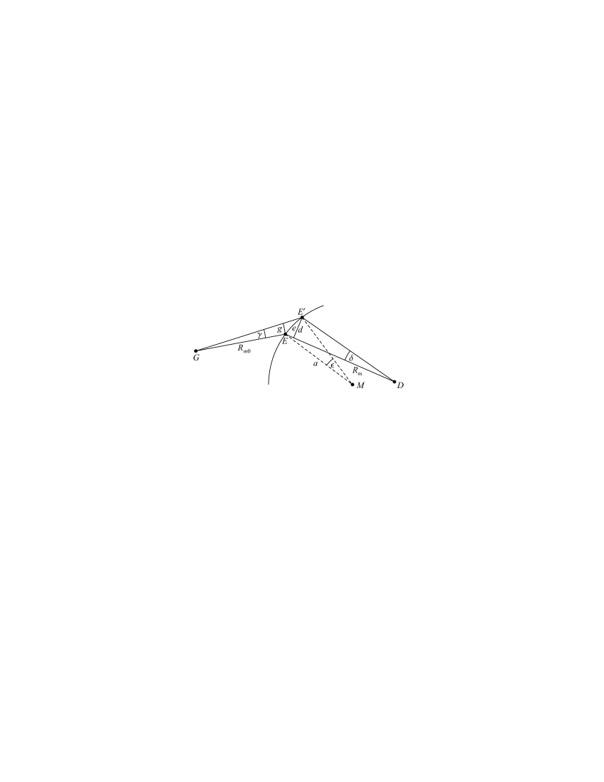
Figure 10: Meridional cross section for the determination of the meridional radius of curvature, $R_{m}$. $M$ is the center of the sphere

The initial radius of curvature is $R_{m0}\equiv\overline{GE}$, the one after refraction is $R_{m}\equiv\overline{ED}$. The infinitesimally neighbored beam ($\gamma\ll 1)$ which is refracted in $E^{\prime}$ (the angles of incidence and transmission in $E$ are $\theta_{i}$ and $\theta_{t}$, in $E^{\prime}$ they be denoted $\theta_{i}^{\prime}$ and $\theta_{t}^{\prime}$) also propagates to $D$. The normals onto $R_{m0}$ through $E$ and onto $R_{m}$ through $E^{\prime}$ are $g$ and $d$, respectively. In the necessary order the length of the arc $EE^{\prime}$ can be approximated by the distance $e\approx\overline{EE^{\prime}}$. As all angles are small: $g=\gamma\,R_{m0}$, $d=\delta\,R_{m}$, and $e=\epsilon\,a$. On the other hand, we find from the infinitesimal triangles: $g=e\cos\theta_{i}$, $d=e\cos\theta_{t}$. This leads to

$$R_{m}=-\dfrac{\gamma\,R_{m0}\cos\theta_{t}}{\delta\cos\theta_{i}}\,,$$ (114)

where we have introduced a minus sign because the wave is converging after the refraction. The remaining problem is the angle $\delta$ in the denominator. To find $\delta$ we write the relations between angles and primed angles:

$$\theta_{i}^{\prime}=\theta_{i}+\gamma+\epsilon\,,\quad\theta_{t}^{\prime}=\theta_{t}-\delta+\epsilon\,.$$ (115)

With Snell’s law

$$\theta_{t}-\theta_{t}^{\prime}=\arcsin\dfrac{\sin\theta_{i}}{n}-\arcsin\dfrac{\sin(\theta_{i}+\gamma+\epsilon)}{n}\,,$$ (116)

a first order Taylor expansion in $(\gamma+\epsilon)$ yields

$$\theta_{t}-\theta_{t}^{\prime}=-\dfrac{(\gamma+\epsilon)\cos\theta_{i}}{n\cos\theta_{t}}\,,$$ (117)

We express $\delta$ from (115), substitute it into (114) and finally obtain the meridional radius of curvature (48)

$$R_{m}=\dfrac{n\,a\,R_{m0}\cos^{2}\theta_{t}}{a\cos^{2}\theta_{i}+R_{m0}\,(\cos\theta_{i}-n\cos\theta_{t})}\,.$$ (118)

For the sagittal radius of curvature we consider figure 11.

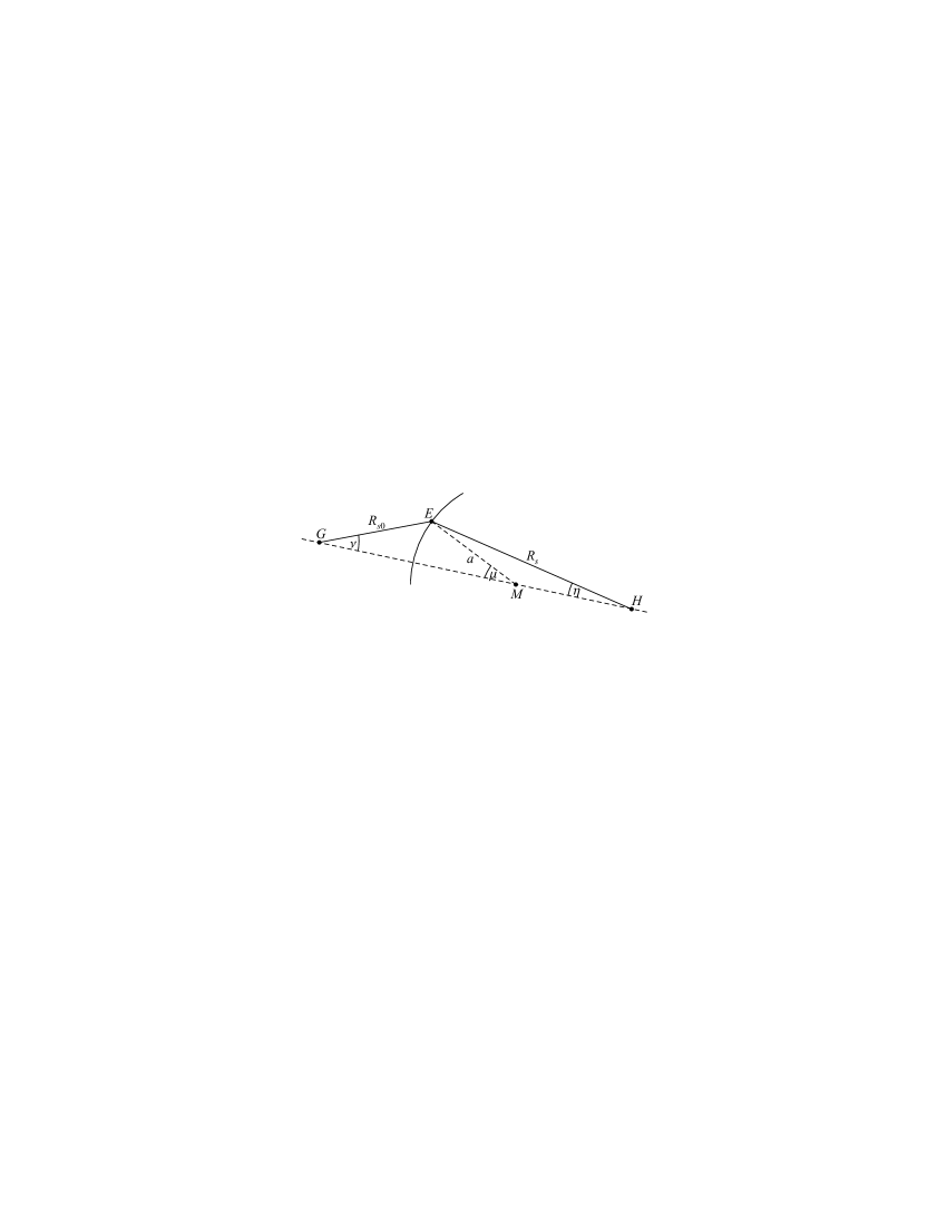
Figure 11: Meridional cross section for the determination of the sagittal radius of curvature, $R_{s}$

A ray which emerged from $G$ is refracted in $E$ (incident angle $\theta_{i}$ and transmitted angle $\theta_{t}$). The distance from $E$ to the intersection $H$ of the ray with the line passing through $G$ and the sphere center $M$ is the sagittal radius of curvature, as a neighbored ray, emerging from $G$ and hitting the sphere not in $E$ but infinitesimally shifted perpendicular to the meridional plane, will also propagate to $H$ due to symmetry around the line $GM$. We have $R_{s0}\equiv\overline{GE}$ and $R_{s}\equiv\overline{EH}$. The tangent theorem states (all angles are in general large now)

$$\tan\dfrac{\nu-\mu}{2}=\dfrac{a-R_{s0}}{a+R_{s0}}\,\cot\dfrac{\pi-\theta_{i}}{2}\,,$$ (119)

where $\pi-\theta_{i}$ is just the third angle in the triangle $GME$. Due to $\nu+\mu=\theta_{i}$ we find

$$\mu=\dfrac{\theta_{i}}{2}-\arctan\!\left(\dfrac{a-R_{s0}}{a+R_{s0}}\,\cot\dfrac{\pi-\theta_{i}}{2}\right)\!.$$ (120)

In the triangle $MHE$ the sine theorem reads

$$-\dfrac{R_{s}}{a}=\dfrac{\sin(\pi-\mu)}{\sin\eta}\,,$$ (121)

where we have again introduced a minus sign due to the convergence of the refracted wave. Trigonometric transformations finally give the sagittal radius of curvature (49)

$$R_{s}=\dfrac{n\,a\,R_{s0}}{a+R_{s0}\,(\cos\theta_{i}-n\cos\theta_{t})}\,.$$ (122)

References

- (1) J. E. G. J. Wijnhoven and W. L. Vos, Science 281, 802 (1998)
- (2) Y. A. Vlasov, X.-Z. Bo, J. C. Sturm, and D. J. Norris, Nature 414, 289 (2001)
- (3) M. L. Gorodetsky, A. A. Savchenkov, and V. S. Ilchenko, Opt. Lett. 21, 453 (1996)
- (4) K. J. Vahala, Nature 424, 839 (2003)
- (5) F. Burmeister, W. Badowsky, T. Braun, S. Wieprich, J. Boneberg, and P. Leiderer, Appl. Surf. Sci. 144, 461 (1999)
- (6) D. Bäuerle, Laser Processing and Chemistry, Springer–Verlag, Edition (2000)
- (7) D. Bäuerle, L. Landström, J. Kofler, N. Arnold, and K. Piglmayer, Proc. SPIE 5339, 20 (2004)
- (8) H.-J. Münzer, M. Mosbacher, M. Bertsch, J. Zimmermann, P. Leiderer, and J. Boneberg, J. Microsc. 202, 129 (2001)
- (9) B. S. Luk’yanchuk (Editor), Laser Cleaning, World Scientific Publishing (2002)
- (10) B. S. Luk’yanchuk, N. Arnold, S. M. Huang, Z. B. Wang, and M. H. Hong, Appl. Phys. A 77, 209 (2003)
- (11) C. F. Bohren and D. R. Huffman, Absorption and Scattering of Light by Small Particles, John Willey Sons (1983)
- (12) G. Roll and G. Schweiger, J. Opt. Soc. Am. A 17, 1301 (2000)
- (13) A. Rohrbach, Phys. Rev. Lett. 95, 168102 (2005)
- (14) W. Zimmer, Nonlinear optical effects by the interaction of femtosecond laser pulses with microdroplets, PhD thesis, Freie Universität Berlin, Germany (2001)
- (15) G. Mie, Ann. d. Physik 25, 377 (1908)
- (16) M. Born and E. Wolf, Principles of Optics, Cambridge University Press, Edition (2002)
- (17) Y. A. Kravtsov and Y. I. Orlov, Caustics, Catastrophes and Wave Fields, Springer Series on Wave Phenomena (Vol. 15), Springer–Verlag, Edition (1999)
- (18) M. V. Berry, J. Phys. A: Math. Gen. 13, 149 (1980)
- (19) M. V. Berry, Physics Today 54(4), 11 (2001)
- (20) T. Pearcey, The structure of an electromagnetic field in the neighbourhood of a cusp of a caustic, Lond. Edinb. Dubl. Phil. Mag. 37, 311 (1946)
- (21) J. N. Connor and D. Farrelly, J. Chem. Phys. 75, 2831 (1981)
- (22) N. P. Kirk, J. N. Connor, P. R. Curtis, and C. A. Hobbs, J. Phys. A: Math. Gen. 33, 4797 (2000)
- (23) I. N. Bronstein and K. A. Semendjajew, Handbook of Mathematics, Springer–Verlag, Edition (2004)
- (24) J. Focke, Optica Acta 3, 110 (1956)
- (25) M. Abramowitz and I. A. Stegun (Editors), Handbook of Mathematical Functions with Formulas, Graphs and Mathematical Tables, John Wiley & Sons (1993)
- (26) D. McGloin and K. Dholakia, Contemporary Physics 46, 15 (2005)
- (27) J. Kofler, Focusing of Light in Axially Symmetric Systems within the Wave Optics Approximation, Master Thesis, Johannes Kepler Universität Linz, Austria (2004)
- (28) In the present work all plots of the Bessoid integral (and its derivatives) contain mesh points, computed with the software package Mathematica 5 (Wolfram Research). Direct numerical integration of (2) takes more than one hour on a modern personal computer. Integration along a line in the complex plane decreases the amount of time by approximately a factor of 3. Solving the ordinary differential equation (12), however, lasts only a few seconds.
- (29) J. N. Connor and P. R. Curtis, J. Math. Phys. 25, 2895 (1984). In this work the term cuspoid stands for the whole family of canonical catastrophe integrals with corank 1, beginning with fold (codimension 1), cusp (2), swallowtail (3) and buttererfly (4), but does not mean the surface of revolution of a cusp with corank 2 and codimension 2 as we use it.
- (30) J. N. Connor, Mol. Phys. 26, 1217 (1973)
- (31) J. J. Stamnes and B. Spjelkavik, Optica Acta 30, 1331 (1983)
- (32) A. J. Janssen, J. Phys. A: Math. Gen. 25, L823 (1992)
- (33) T. Pearcey and G. W. Hill, Spherical aberrations of second order: the effect of aberrations upon the optical focus, Melbourne: Commonwealth Scientific and Industrial Research Organization, 71 (1963)
- (34) Y. A. Kravtsov and Y. I. Orlov, Geometrical Optics of Inhomogeneous Media, Springer Series on Wave Phenomena (Vol. 6), Springer–Verlag (1990)
- (35) L. M. Brekhovskikh and O. A. Godin, Acoustics of Layered Media II, Springer Series on Wave phenomena (Vol. 10), Springer–Verlag (1992)
- (36) L. Bergmann and C. Schäfer, Lehrbuch der Experimentalphysik (Band 3, Optik), Hrsg: H. Gobrecht, Verlag Walter de Gruyter, 7. Auflage (1978)
- (37) V. Červený, Seismic Ray Theory, Cambridge University Press (2001)
- (38) J. B. Keller, J. Opt. Soc. Am. 52, 116 (1962)
- (39) D. Bäuerle, G. Wysocki, L. Landström, J. Klimstein, K. Piglmayer, and J. Heitz, Proc. SPIE 5063, 8 (2003)
- (40) G. Langer, Micro- and Nanopatterning by Means of Colloidal Monolayers, Master Thesis, Johannes Kepler Universität Linz, Austria (2005)
- (41) R. Dorn, S. Quabis, and G. Leuchs, Phys. Rev. Lett. 91, 233901 (2003)
- (42) A. D. Peters, C. Jaffé, J. Gao, and J. B. Delos, Phys. Rev. A 56, 345 (1997)
- (43) P. V. Parimi, W. T. Lu, P. Vodo, and S. Sridhar, Nature 426, 404 (2003)
- (44) M. V. Berry and M. R. Jeffrey, J. Opt. A: Pure Appl. Opt. 8, 363 (2006)
- (45) J. F. Nye, J. Opt. A: Pure Appl. Opt. 7, 95 (2005)
- (46) D. Bäuerle, K. Piglmayer, R. Denk, and N. Arnold, Lambda Physik 60, 1 (2002)
- (47) M. V. Berry, I. Marzoli, and W. Schleich, Physics World 14(6), 39 (2001)