Strong-field ionization of atoms and molecules: The two-term saddle point method

Abstract

We derive an analytical formula for the ionization rate of neutral atoms and molecules in a strong monochromatic field. Our model is based on the strong-field approximation with transition amplitudes calculated by an extended saddle point method. We show that the present two-term saddle point method reproduces even complicated structures in angular resolved photo electron spectra.

I Introduction

In order to describe fully the dynamics of molecules and atoms subject to an external laser field, one must in principle solve the time dependent Schrödinger equation including all degrees of freedom. Such ab initio solutions are, however, impossible for any but the most simple systems, and additionally these methods are often only available for a few specialized theoretical research groups. Fortunately much physical insight can be achieved by simpler models. For example, many strong-field phenomena can be successfully interpreted if one uses the Ammosov-Delone-Krainov (ADK) tunneling model Ammosov et al. (1986) to describe ionization. The success and the analytical simplicity makes the ADK model ideal for widespread use not only for atoms but also for diatomic Tong et al. (2002) and polyatomic Kjeldsen et al. (2005) molecules.

Along with the ADK model, the strong-field approximation (SFA) is one of the most widely used models to describe detachment of anions and ionization of atoms in intense laser fields. Compared with the ADK model, the SFA is more suited for obtaining angular and energy resolved spectra. The two models are in fact connected since the tunneling rate can be obtained from the SFA in the low frequency limit Perelomov et al. (1966); Gribakin and Kuchiev (1997). The initial work by Keldysh Keldysh (1965) concerned ionization of hydrogen. The model was further developed by Faisal and Reiss Faisal (1973); Reiss (1980) and is commonly known as the Keldysh-Faisal-Reiss (KFR) model. Later on, the model was extended in various ways (see Ref. Becker and Faisal (2005) for a recent review), e.g., to take into account rescattering Milošević and Ehlotzky (1998); Gazibegovic-Busuladzic et al. (2004), long range Coulomb potential in the final state Duchateau et al. (2002), multiple electrons Becker and Faisal (2000, 2002) and molecular structure Muth-Böhm et al. (2000). More systematically, for short-ranged final state interactions the SFA transition amplitude is the leading term in an exact S-matrix series Reiss (1980); Becker and Faisal (2005).

In order to evaluate the matrix elements that enter the expression for the ionization rate in the SFA, one may use the saddle point method to obtain approximate closed analytical formulas. The saddle point method can be applied in both the length- and velocity gauge. In the velocity gauge, the saddle point method breaks down at intensities below $10^{13}\,\mbox{W/cm}^{2}$ Requate et al. (2003). Despite its wide-spread and long-term use – already Keldysh applied the saddle point method in the initial work concerned with the limit of small momenta of the outgoing electron and Ref. Popov (2004) reviews other limiting formulas – we are not aware of a similar study of the limitation of the saddle-point method in the length gauge. The main purpose of the present paper is to provide a detailed discussion of the applicability of the saddle point method in neutral atoms and to extend the theory to cover molecules. In this effort, we identify a straightforward extension of the conventional saddle point method. We call the extended theory the ’two-term’ saddle point method, and we show that the present method increases the accuracy considerably.

The paper is organized as follows. In Sec. II we outline the theory. In Sec. III we test the accuracy of the saddle point method by presenting result on various atoms and molecules. Section IV concludes.

II Theory

The saddle point method gives very accurate results for detachment rates of negative ions Gribakin and Kuchiev (1997); Figueira de Morisson Faria et al. (2002) and a saddle point formula that covers also neutral atoms, irrespectively of the value of the momentum of the outgoing electron, is known Gribakin and Kuchiev (1997). The application of the latter formula, however, was not considered until recently Ostrovsky and Greenwood (2005); Ostrovsky (2005). The theory outlined here follows closely the derivation of Ref. Gribakin and Kuchiev (1997). The differences are that (i) we take into account molecular structure, and (ii) the previous theory only included one term in saddle-point evaluation of a particular integral, whereas we keep two terms to increase the accuracy and range of applicability [see Eq. (14) below]. Equations (1)-(4) below summarize the basic formulas from Ref. Gribakin and Kuchiev (1997) and are included here for completeness.

In the single-active-electron approximation, we consider the direct transition of the electron in an initially bound state $\Psi_{0}$ to a continuum state $\Psi_{\bm{q}}$ due to the linearly polarized laser field $\bm{F}(t)=\bm{F}_{0}\cos(\omega t)$ with the period $T=2\pi/\omega$. We quote the expression for the angular differential ionization rate (atomic units $\hbar=m_{e}=|e|=1$ with the electron charge $e=-1$ are used throughout)

$$\frac{dW}{d\Omega}=\frac{1}{(2\pi)^{2}}\sum_{n=n_{\textrm{min}}}^{\infty}|A_{\bm{q}n}|^{2}q_{n},$$ (1)

with the transition amplitude for the $n$-photon process

$$A_{\bm{q}n}=\frac{1}{T}\int_{0}^{T}\langle\Psi_{\bm{q}}({\bm{r}},t)|\bm{F}(t)\cdot\bm{r}|\Psi_{0}({\bm{r}},t)\rangle dt,$$ (2)

which is to be calculated at the momentum $q_{n}=\sqrt{2(n\omega-E_{b}-U_{p})}$, with $E_{b}$ the binding energy of the initial bound electron and $U_{p}=F_{0}^{2}/(4\omega^{2})$ the ponderomotive potential. Since the final momentum is real, a minimum number of photons $n_{\textrm{min}}$ must be absorbed. In the SFA, the interaction between the field and the electron in the initial state $\Psi_{0}(\bm{r},t)$ is neglected and accordingly $\Psi_{0}(\bm{r},t)=\Phi_{0}(\bm{r})\exp{(iE_{b}t)}$, where $\Phi_{0}(\bm{r})$ is the stationary solution of the field-free Schrödinger equation. Additionally, interactions between the residual ion and the continuum electron are neglected in the final state which is then described by a Volkov wave

$$\Psi_{\bm{q}}(\bm{r},t)=\exp\left\{i[\bm{q}+\bm{A}(t)]\cdot\bm{r}-\frac{i}{2}\int^{t}[\bm{q}+\bm{A}(t^{\prime})]^{2}dt^{\prime}\right\},$$ (3)

with the vector potential $\bm{A}(t)=-\bm{F}_{0}/\omega\sin(\omega t)$. We omit the lower integration limit corresponding to an adiabatical turn-on of the field at $t\rightarrow-\infty$.

Following Ref. Gribakin and Kuchiev (1997) we write the transition amplitude equivalently as

$$A_{\bm{q}n} = \frac{1}{T}\int_{0}^{T}\frac{-\kappa^{2}-[\bm{q}+\bm{A}(t)]^{2}}{2}\tilde{\Phi}_{0}[\bm{q}+\bm{A}(t)]$$ (4)

$$\times \exp\left[i\int^{t}\frac{[\bm{q}+\bm{A}(t^{\prime})]^{2}+\kappa^{2}}{2}dt^{\prime}\right]dt,$$

with $\kappa=\sqrt{2E_{b}}$ and $\tilde{\Phi}_{0}(\bm{q})$ being the Fourier transform of $\Phi_{0}(\bm{r})$. The transition into the continuum takes place at large distances from the ionic core, and hence, for the initial state, it is accurate to use the asymptotic Coulomb form which we expand in partial waves

$$\Phi_{0}(\bm{r})\sim\sum_{lm}C_{lm}r^{\nu-1}e^{-\kappa r}Y_{lm}({\hat{\bm{r}}}),$$ (5)

with $\nu=Z/\kappa$ and $Z$ the charge of the residual ion. Here we assume a general non-spherically symmetric potential. For atoms, only one term contributes and for linear molecules in the body fixed frame, we only include $m$ states corresponding to the projection of the angular momentum on the internuclear axis. We determine the asymptotic expansion coefficients $C_{lm}$ by matching the Hartree-Fock orbital of the most loosely bound electron to the form of Eq. (5) Kjeldsen and Madsen (2005). The Fourier transform of Eq. (5) is

$$\tilde{\Phi}_{0}(\bm{q}) = \sum_{lm}C_{lm}4\pi\left(-\frac{iq}{\kappa}\right)^{l}\frac{\sqrt{\pi}\kappa^{\nu}\Gamma(l+\nu+2)}{2^{l+1}\Gamma(l+\frac{3}{2})(\kappa^{2}+q^{2})^{\nu+1}}$$ (6)

$$\times F\left(\frac{l-\nu}{2},\frac{l-\nu+1}{2};l+\frac{3}{2};-\frac{q^{2}}{\kappa^{2}}\right)Y_{lm}(\hat{\bm{q}}),$$

where $F(a,b;c;z)$ is Gauss’ hypergeomtric series. We insert the Fourier transform above in Eq. (4) and obtain

$$A_{\bm{q}n} = -\frac{1}{T}\int_{0}^{T}\sum_{lm}C_{lm}\left[\frac{Q(t)}{i\kappa}\right]^{l}\frac{2^{1-l}\pi^{3/2}\kappa^{\nu}\Gamma(l+\nu+2)}{\Gamma(l+\frac{3}{2})[Q(t)^{2}+\kappa^{2}]^{\nu}}$$ (7)

$$\times F\left(\frac{l-\nu}{2},\frac{l-\nu+1}{2};l+\frac{3}{2};-\frac{Q(t)^{2}}{\kappa^{2}}\right)Y_{lm}[\hat{\bm{Q}}(t)]$$

$$\times e^{iS(t)}dt,$$

with kinematical momentum $\bm{Q}(t)=\bm{q}+\bm{A}(t)$, and action

$$S(t) = \int^{t}\frac{Q(t^{\prime})^{2}+\kappa^{2}}{2}dt^{\prime}$$

$$= n\omega t+\frac{\bm{q}\cdot\bm{F}_{0}}{\omega^{2}}\cos(\omega t)-\frac{U_{p}}{2\omega}\sin(2\omega t).$$

In a multiphoton process $n\gg 1$ and the exponential factor $e^{iS(t)}$ therefore oscillates rapidly on the interval $0\leq t\leq T$. This fact makes the integral difficult to evaluate directly from Eq. (7).

The time integral of Eq. (7) follows obviously the real $t$ axis. From Eq. (7) and the convergence of the hypergeomtric function, we see that the integrand is an analytical function of $t$ except at complex instants of time satisfying

$$[\bm{q}+\bm{A}(t)]^{2}=Q(t)^{2}=-\kappa^{2},$$ (9)

where $\tilde{\Phi}_{0}[\bm{q}+\bm{A}(t)]$ is singular. These points coincide with the saddle points $S^{\prime}(t)=0$ in the factor $e^{iS(t)}$. We discuss the complex momentum in appendix A and refer to Refs. Gazibegovic-Busuladzic et al. (2004); Gribakin and Kuchiev (1997) for the analytical properties and evaluation of the spherical harmonics on a complex vector. The continuation to the complex $t$ plane is straightforward as long as we remember to treat the singularities with care. Note that the singularities vanish when $\nu=Z=0$ corresponding to detachment of negative ions. In Fig. 1 we show the integrand of Eq. (7) for a typical set of laser parameters applied to the ground state of hydrogen ($l=m=0,C_{00}=2$). The integral along the closed contour shown in Fig. 1 is zero according to Cauchy’s theorem since we carefully avoid to enclose the singularities marked by crosses. The integrand is clearly invariant under the periodic translation ${\rm Re}(t)+i{\rm Im}(t)\rightarrow{\rm Re}(t+T)+i{\rm Im}(t)$. Hence, the contributions to the integral from the vertical paths $\mathcal{P}_{2}$ and $\mathcal{P}_{4}$ cancel exactly and, consequently, the contributions along the horizontal paths must also cancel. We can therefore equally well evaluate the integral Eq. (7) along the negative $\mathcal{P}_{3}$ path.

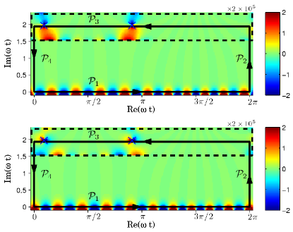
Figure 1: (Color online) Integration contour. Upper (lower) panel: real (imaginary) part of the oscillating factor $e^{iS(t)}$. In the regions bounded by dashed squares, function values are multiplied by $2\times 10^{5}$ ($\textrm{Im}(\omega t)>1.5$). The parameters correspond to ionization of hydrogen in the polarization direction by 10 photons at $800\,\mbox{nm}$ at an intensity of $1\times 10^{13}\,\mbox{W/cm}^{2}$.

At the expense of introducing complex and unphysical times, we see from Fig. 1 that we can calculate the integral more efficiently in the complex $t$ plane. It is apparently much easier to evaluate the integral along the path $-\mathcal{P}_{3}$ than along the real axis $\mathcal{P}_{1}$. Along the former path, the factor $e^{iS(t)}$ is nearly zero everywhere except at the two saddle points while the same factor oscillates along the entire path $\mathcal{P}_{1}$. This fact is of course the basis for any asymptotic expansion. Strictly speaking, the saddle point method requires that we deformate the path to pass across the saddle point in the direction of the steepest descent. In practice, the required deformation from the horizontal line is small and has negligible influence on the final results.

In the saddle point method outlined in Ref. Gribakin and Kuchiev (1997), one neglects the variations of $\bm{Q}(t)$ over the range where the factor $[Q(t)^{2}+\kappa^{2}]^{-\nu}e^{iS(t)}$ has a significant amplitude, i.e., according to Eq. (9) we let $Q(t)=\pm i\kappa$ in the remaining factors and obtain

$$A_{\bm{q}n} \approx -\sum_{lm}C_{lm}\Gamma(\nu+1)\left(\frac{\kappa}{\omega}\right)^{\nu}\sum_{\mu=1,2}(\pm 1)^{l}Y_{lm}(\hat{\bm{q}}_{\mu})$$ (10)

$$\times \int_{-\mathcal{P}_{3}^{\mu}}\frac{e^{iS(\phi)}}{[S^{\prime}(\phi)]^{\nu}}d\phi,$$

where $\phi=\omega t$ and $S^{\prime}(\phi)=[Q(t)^{2}+\kappa^{2}]/(2\omega)$. We expect such an approximation to be most accurate for $l=0$ since the factors $Q(t)^{l}Y_{lm}[\hat{\bm{Q}}(t)]$ in Eq. (7) are constant in this case. The integrals are to be evaluated along the negative direction of the path $\mathcal{P}_{3}$ near the $\mu$’th point of stationary phase. In Ref. Gribakin and Kuchiev (1997), the denominator was expanded as

$$[S^{\prime}(\phi)]^{-\nu}\approx[S^{\prime\prime}(\phi_{\mu})]^{-\nu}(\phi-\phi_{\mu})^{-\nu},$$ (11)

near the saddle points. As we show in Sec. III.1 below, we obtain higher accuracy if we expand $S^{\prime}(\phi)$ to second order around the saddle point

$$S^{\prime}(\phi)\approx S^{\prime\prime}(\phi_{\mu})(\phi-\phi_{\mu})\left[1+\frac{S^{(3)}(\phi_{\mu})}{2S^{\prime\prime}(\phi_{\mu})}(\phi-\phi_{\mu})\right],$$ (12)

and by the first order binomial series

$$[S^{\prime}(\phi)]^{-\nu} \approx [S^{\prime\prime}(\phi_{\mu})]^{-\nu}(\phi-\phi_{\mu})^{-\nu}$$ (13)

$$-\nu\frac{S^{(3)}(\phi_{\mu})}{2[S^{\prime\prime}(\phi_{\mu})]^{\nu+1}}(\phi-\phi_{\mu})^{-\nu+1}.$$

With this expansion inserted in Eq. (10), the integral now becomes a sum of two terms

$$\int_{-\mathcal{P}_{3}^{\mu}}\frac{e^{iS(\phi)}d\phi}{[S^{\prime}(\phi)]^{\nu}}\approx\mathcal{I}_{0\mu}(1+\mathcal{C_{\mu}}),$$ (14)

with the conventional saddle-point term

$$\mathcal{I}_{0\mu} = [S^{\prime\prime}(\phi_{\mu})]^{-\nu}\int_{-\mathcal{P}_{3}^{\mu}}\frac{e^{iS(\phi)}}{(\phi-\phi_{\mu})^{\nu}}d\phi$$ (15)

$$\approx \frac{i^{\nu}\Gamma(\frac{\nu}{2})}{2\Gamma(\nu)}\left[\frac{-2i}{S^{\prime\prime}(\phi_{\mu})}\right]^{\frac{\nu}{2}}\left[\frac{2\pi i}{S^{\prime\prime}(\phi_{\mu})}\right]^{\frac{1}{2}}e^{iS(\phi_{\mu})}$$

and the present correction term

$$\mathcal{C}_{\mu} = -\frac{1}{\mathcal{I}_{0}}\frac{\nu S^{(3)}(\phi_{\mu})}{2[S^{\prime\prime}(\phi_{\mu})]^{\nu+1}}\int_{-\mathcal{P}_{3}^{\mu}}\frac{e^{iS(\phi)}}{(\phi-\phi_{\mu})^{\nu-1}}d\phi$$ (16)

$$\approx \frac{\nu S^{(3)}(\phi_{\mu})}{(2i)^{1/2}S^{\prime\prime}(\phi_{\mu})^{3/2}}\frac{\Gamma\left(\frac{\nu+1}{2}\right)}{\Gamma\left(\frac{\nu}{2}\right)}.$$

In Eqs. (15) and (16), we extended the integration limits to infinity and used the asymptotic approximation Gribakin and Kuchiev (1997)

$$\int\frac{e^{iS(\phi)}d\phi}{(\phi-\phi_{\mu})^{\nu}}\approx\frac{i^{\nu}\Gamma(\frac{\nu}{2})}{2\Gamma(\nu)}\left[\frac{2\pi i}{S^{\prime\prime}(\phi_{\mu})}\right]^{\frac{1}{2}}[-2iS^{\prime\prime}(\phi_{\mu})]^{\frac{\nu}{2}}e^{iS(\phi_{\mu})}.$$ (17)

$\mathcal{I}_{0\mu}$ recovers the result of Ref. Gribakin and Kuchiev (1997) while $\mathcal{C_{\mu}}$ is a correction that arizes from the higher order expansion of $[S^{\prime}(\phi)]^{-\nu}$. We present the main formula of the present work in the next equation

$$A_{\bm{q}n}\approx-\sum_{lm}C_{lm}\Gamma(\nu+1)\left(\frac{\kappa}{\omega}\right)^{\nu}\sum_{\mu=1,2}(\pm 1)^{l}Y_{lm}(\hat{\bm{q}}_{\mu})\times\left\{\begin{array}[]{ll}{\cal I}_{0\mu}(1+{\cal C}_{\mu})&\mbox{two-term}\\ {\cal I}_{0\mu}&\mbox{one-term}\end{array}\right..$$ (20)

With the inclusion of ${\cal I}_{0\mu}(1+{\cal C}_{\mu})$, we refer to Eq. (20) as the two-term saddle point approximation while neglecting $\mathcal{C}_{\mu}$ and maintaining only ${\cal I}_{0\mu}$ in (20) is referred to as the one-term saddle point approximation. We note from Eq. (16) that there is no significant additional numerical complications involved with the inclusion of the second term.

We find $\phi_{\mu}$ from the saddle point conditions of Eq. (LABEL:eqn:action)

$$S^{\prime}(\phi_{\mu})=n-z+\xi\sin\phi_{\mu}+2z\sin^{2}\phi_{\mu}=0,$$ (21)

with $\xi=-\bm{F}_{0}\cdot\bm{q}/\omega^{2}$ and $z=U_{p}/\omega$. The solutions to Eq. (21) are

$$\sin\phi_{\mu}=\frac{-\xi\pm i\sqrt{8z(n-z)-\xi^{2}}}{4z},$$ (22)

from which it follows that

$$\cos\phi_{\mu} = \pm\sqrt{1-\sin^{2}\phi_{\mu}}$$ (23)

$$e^{iS(\phi_{\mu})} = (\cos\phi_{\mu}+i\sin\phi_{\mu})^{n}e^{-i\cos\phi_{\mu}(\xi+z\sin\phi_{\mu})}$$ (24)

$$S^{\prime\prime}(\phi_{\mu}) = \cos\phi_{\mu}(\xi+4z\sin\phi_{\mu})$$ (25)

$$S^{(3)}(\phi_{\mu}) = -\xi\sin\phi_{\mu}+4z[2\cos^{2}\phi_{\mu}-1],$$ (26)

where the signs correspond to $Q(t_{\mu})=\mp i\kappa$ at the saddle points. We combine Eqs. (10), (14)-(16) and (22)-(26) to obtain the analytical approximation to the transition amplitude, Eq. (7).

The inclusion of nuclear motion in the molecular case was discussed in detail for ionization Kjeldsen and Madsen (2005) and for high harmonic generation Madsen and Madsen (200X) within the SFA. The form of the amplitude (7) stays the same and the formulas are straightforwardly generalized. When it comes to the assessment of the accuracy of the saddle-point method which is the main objective of the present paper, nuclear motion is unimportant and is left out for clarity.

III Results

III.1 Test case: atomic hydrogen

First we consider ionization of ground state hydrogen. We use this system to benchmark the accuracy of the saddle point method against numerical integration. The atomic structure parameters are $C_{00}=2$, $\kappa=1$ and $\nu=1$. Furthermore, the asymptotic form of Eq. (5) is identical to the exact wave function at all distances and the Fourier transform is

$$\tilde{\Phi}_{0}(\bm{q})=\frac{16\pi}{(1+q^{2})^{2}}\frac{1}{\sqrt{4\pi}}.$$ (27)

The spherical harmonic and the hypergeomtric function in Eq. (7) are both constant and it is therefore exact to neglect variations therein around the saddle point when we derive Eq. (10).

After choosing the alternative integration path $-\mathcal{P}_{3}$ of Fig. 1, the transition amplitude reduces to

$$A_{\bm{q}n}=-\frac{8\pi}{\sqrt{4\pi}\omega}\frac{1}{2\pi}\times\sum_{\mu=1,2}\left\{\begin{array}[]{ll}{\cal I}_{0\mu}(1+{\cal C}_{\mu})&\mbox{two-term}\\ {\cal I}_{0\mu}&\mbox{one-term}\end{array}\right.$$ (30)

Here we test the accuracy of Eq. (20) [or (30)], and in particular the difference between the one-term (only ${\cal I}_{0\mu}$ included) and the two-term (${\cal I}_{0\mu}(1+{\cal C}_{\mu})$ included) saddle point formulas.

Figure 2: (a) Real and (b) imaginary parts of the integrand $e^{iS(\phi)}[S^{\prime}(\phi)]^{-\nu}$ along the integration path $-\mathcal{P}_{3}$ in the neighborhood of the second saddle-point in Fig. 1, solid. The long dashed line is the approximation around the second saddle point including only ${\cal I}_{0\mu}$. The two-term approximation including ${\cal I}_{0\mu}(1+{\cal C}_{\mu})$ is the short dashed line which overlaps completely the solid line. The parameters of the laser are as in Fig. 1.

In Fig. 2 we show the integrand along the integration path in the neighborhood of the second saddle point (see Fig 1). Additionally, we show the results of the approximations using the one- and two-term expansion around the second saddle point in Eq. (13). We see that the one-term expansion recovers quite well the peak structure around the saddle point. In the wings of the peak, the two-term expansion is significantly better, which is most evident from the real part of the integrand, panel (a). We have integrated the integral numerically and obtained the value $5.64\times 10^{-8}$ while we obtain the values $4.55\times 10^{-8}$ and $5.39\times 10^{-8}$ for the one- and two-term saddle point approximation, Eq. (14) summed over the two saddle points.

Figure 3: (a)-(d) Angular differential ionization rate of hydrogen for the lowest number of photon absorptions, $n=10-13$ ordered by increasing $n$. The solid curve is obtained by numerical integration while long and short dashed curves are obtained by the saddle point method with the one- and two-term approximation, respectively. The laser wavelength is $800\,\mbox{nm}$ and the intensity is $1\times 10^{13}\,\mbox{W/cm}^{2}$.

Having seen that the saddle point method is accurate in the single case above, namely ionization parallel to the field by 10 photons, we now present the $n$-photon angular differential rates at varying photon orders in Fig. 3. Here $\theta_{q}$ is the polar angle of the outgoing electron with respect to the polarization axis. Figure 3 shows that both saddle point methods predict an angular structure in close agreement with the numerical integration. The rates obtained by the single-term approximation are, however, around $35\%$ too small. The two-term approximation is significantly better with an accuracy within $10\%$.

In our final test, we consider the total ionization rate integrated over all angles of the outgoing electron. In Fig. 4 (a) we present total ionization rates at $800\,\mbox{nm}$ obtained with the numerical integration and the one- and two-term saddle point approximation. All three methods produce results in quite good agreement over many orders of magnitude on the scale shown in the figure. In order to investigate the accuracy of the saddle point method in some more detail, we calculate the ratio $W_{\textrm{saddle}}/W_{\textrm{num}}$ between the rates obtained by the saddle point method and the numerical integration. Figures 4 (b) and (c) present the results for various wavelengths and intensities.

Figure 4: (a) Absolute rates at a wavelength of $800\,\mbox{nm}$. The result of numerical integration is indicated by the solid line while the long- and short dashed lines are the one- and two-term saddle point approximation, respectively. (b) and (c) Ratio between total ionization rates obtained by the saddle point method and numerical integration for varying wavelength and intensity. We show saddle point results for the one- and two-term approximation in panels (b) and (c), respectively.

Again, we use both the one- and two-term approximation, i.e., we study the results of Eq. (20) with ${\cal I}_{0\mu}$ and ${\cal I}_{0\mu}(1+{\cal C}_{\mu})$, respectively. First, we see that the accuracies of both saddle point methods are nearly independent of the intensity for each fixed value of the wavelength. From panel (b) we note that the results of the one-term approximation depend significantly on the wavelength. The error is up to a factor of two for the shortest wavelength $248\,\mbox{nm}$ while the error decreases with increasing wavelength. The two-term approximation, on the other hand, produces much more accurate results, panel (c). The rates are approximately $10\%$ too small for all intensities and wavelengths considered. Even though the simple single-term saddle point approximation is somewhat poorer than the two-term approximation the error in the hydrogenic case is approximately constant over twelve orders of magnitude and is not expected to be of major significance compared with the approximations in the SFA itself. In the rest of the paper, we use only the two-term saddle point formula.

III.2 Ionization of atoms

In this section we show results for the noble gas atoms where the active electron initially occupies an orbital in the filled p shell. We calculate the rates for each of the states $m=-1,0,1$ and multiply the result by two corresponding to two equivalent electrons in each orbital. We take the atomic structure parameters $C_{lm}$ and $E_{b}$ from Ref. Kjeldsen and Madsen (2005).

Figure 5: (a) Absolute rates for argon at a wavelength of $800\,\mbox{nm}$. The results of numerical integration are indicated by the solid lines while the short dashed lines are the two-term saddle point approximation. The upper and lower sets of curves are for $m=0$ and $m=1$, respectively. (b) Ratio between total ionization rates from the $m=0$ state obtained by the saddle point method and numerical integration for varying wavelength and intensity. (c) Similar to (b) for the $m=1$ state.

In Fig. 5 we present the absolute and relative rates for the argon atom. As in the case of hydrogen, the saddle point method is accurate over many orders of magnitude, Fig. 5 (a). Interestingly, the saddle point method is slightly better for the $m=1$ [panel (c)] state compared with the $m=0$ state [panel (b)]. This $m$-dependent accuracy turns out to be important in the molecular case as we show in Sec. III.3 below.

Figure 6: Left (right) column: Angular differential rate for argon in the $m=0$ ($m=1$) state. Solid lines are obtained by numerical integration while the dashed lines are by the two-term saddle point method. The laser wavelength is $800\,\mbox{nm}$ and the intensities are (a)-(b) $1\times 10^{13}\,\mbox{W/cm}^{2}$, (c)-(d) $1\times 10^{14}\,\mbox{W/cm}^{2}$ and (e)-(f) $3\times 10^{14}\,\mbox{W/cm}^{2}$

Figure 6 shows angular differential rates summed over all photon absorptions at a wavelength of $800\,\mbox{nm}$ for different intensities. We show the results for both the $m=0$ and $m=1$ state and again we see that the saddle point method works better for the $m=1$ state. The general features in the angular spectra are, however, very well reproduced in all cases.

We mention in closing that the results for krypton and xenon are very similar to argon and are therefore omitted here for brevity.

III.3 Ionization of molecules

In the molecular case, the calculations are most conveniently performed in the laboratory fixed frame with the $z$ axis parallel to the laser polarization. Accordingly, we must express the initial wave function in this frame. The wave function and asymptotic expansion coefficients $C_{lm}$ are, however, most naturally expressed in the body-fixed molecular frame. If the body-fixed frame is rotated by the Euler angles $(\alpha,\beta,\gamma)$ with respect to the laser polarization, we rotate the wave function into the laboratory fixed frame by the rotation operator $\Phi_{0}(\bm{r})\rightarrow D(\alpha,\beta,\gamma)\Phi_{0}(\bm{r})$. The rotation operation effectively allows us to express the asymptotic coefficients in the laboratory frame (LF) by the corresponding coefficients in the molecular frame (MF)

$$C_{lm}^{\text{LF}}=\sum_{m^{\prime}=-l}^{l}\mathscr{D}^{(l)}_{mm^{\prime}}(\alpha,\beta,\gamma)C_{lm^{\prime}}^{\text{MF}},$$ (31)

where $\mathscr{D}^{(l)}_{m^{\prime}m}(\alpha,\beta,\gamma)$ is a Wigner rotation function Zare (1988); Brink and Satchler (1968). For linear polarization and the linear molecules considered in the present work, we only need to consider rotation by the angle $\beta$ between the molecular and field axes. We refer to Ref. Kjeldsen and Madsen (2005) for the coefficients $C_{lm}^{\text{MF}}$.

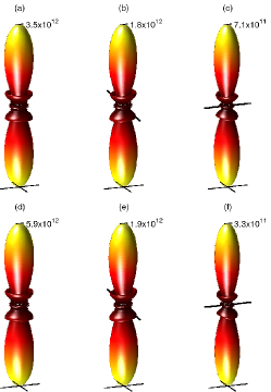
Figure 7: (Color online) Angular differential ionization rate for N₂ aligned at an angle of $0^{\circ}$ [(a) and (d)], $45^{\circ}$ [(b) and (e)], and $90^{\circ}$ [(c) and (f)] with respect to the polarization. Panels (a)-(c) are obtained by numerical integration and panels (d)-(f) by the two-term saddle point method. In all panels, the polarization direction is vertical. In panels (a) and (d) the molecular axis is along the vertical polarization. In the other panels the orientation of the molecular axis is indicated by the line through the origin. All three coordinate axes are scaled equally and the rates are given in units of $\mbox{s}^{-1}$ on the scale indicated in each panel. The laser wavelength is $800\,\mbox{nm}$ and the intensity $2\times 10^{14}\,\mbox{W/cm}^{2}$.

Figure 7 presents angular differential rates for differently aligned N₂ molecules which ionize from the doubly occupied $3\sigma_{g}$ orbital. We show both numerical [(a)-(c)] and two-term saddle point results [(d)-(f)]. First we note that the two methods agree perfectly on the shape of the angular distribution for all alignment angles, $\beta$. The structures are also in good agreement with Ref. Kjeldsen and Madsen (2004), where we used an atomic centred Gaussian basis expansion for the initial state and calculated the transition amplitude numerically. Secondly, the overall structure is nearly independent of $\beta$. The angular rate is simply much favoured along the polarization direction in all geometries. This observation agrees well with the predictions of tunneling theory where the electron by assumption escapes along the polarization axis (For Keldysh parameter $\gamma=\kappa\omega/F_{0}\ll 1$, the ionization dynamics is tunneling like. In Fig. 7, $\gamma=0.81$, i.e., approaching the tunneling regime.)

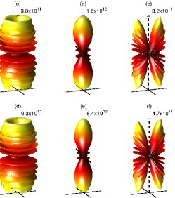
Figure 8: (Color online) Similar to Fig. 7 but for O₂.

Figure 8 shows the angular differential rate for O₂ which ionizes from the two half-filled degenerate $\pi_{g}$ orbitals, one with $m=1$ and one with $m=-1$. We show the results for a single electron with projection $m=1$ and note that the rate is similar for $m=-1$. Again we see that the two methods predict the exact same complex angular structures. The structures can be understood from the symmetry of the initial wave function. The initial $\pi_{g}$ orbital has zero amplitude along- and in the plane perpendicular to the molecular axis and the nodal structure of the wave function forbids the electron to be emitted along the vertical polarization axis when this axis coincides with a nodal plane Kjeldsen et al. (2005).

In Figs. 7 and 8 we see that even though the angular structures agree perfectly, the absolute scales differ by up to a factor of four. We therefore finally turn to a discussion of the alignment dependent rate. We calculate the total rate integrated over all angles of the outgoing electron and show the results in Fig. 9.

Figure 9: Alignment dependent ionization rates for (a) N₂ and (b) O₂. The solid lines are obtained by numerical integration and the dashed line by the two-term saddle point method. The parameters of the laser are as in Fig. 7.

The figure shows that both methods agree that the rate for N₂ is maximized when the molecule is aligned parallel to the polarization axis ($\beta=0$) and minimized when aligned perpendicularly ($\beta=90^{\circ}$). Such an alignment dependence is also seen experimentally Litvinyuk et al. (2003). For O₂ both methods also agree that the rate is maximized around an alignment angle of $40^{\circ}$. For both molecules, however, the two-term saddle point method predicts a too large variation compared with the numerical integration. The reason for this disagreement lies in the $m$-dependent accuracy of the saddle point method as we discussed in Sec. III.2. When we rotate a molecule we change the expansion of the initial wave function in the laboratory fixed spherical harmonics. The rotation operation mixes the different $m$-states according to Eq. (31). Since the part of the transition amplitude that corresponds to each of the $m$-states can be either slightly too large or too small by the saddle point method, the overall accuracy depends on the partial wave decomposition after the rotation. For the atomic $l=1$ and $m=0,\pm 1$ states of Sec III.2, the two-term saddle point method is still quite accurate and the small differences reported there compared with the numerical integration cannot account for the disagreement between the two methods in Fig. 9. For the molecules, however, we have included angular momentum states up to $l=4$ and it turns out that the saddle point method becomes increasingly inaccurate with increasing $l$. If the active electron initially occupies an orbital with a component of non-zero angular momentum, we expect the saddle point method to be somewhat poorer than for $l=0$ as we discussed in deriving Eq. (10). In Eq. (10), we evaluate the factors $Q(t)^{l}Y_{lm}[\hat{\bm{Q}}(t)]$ and the hypergeomtric function at the saddle points. This approximation is naturally most accurate if $\bm{Q}(t)$ is nearly constant in the vicinity of the saddle points. In appendix A, we calculate $Q(t)$ along the integration contour and we see from Fig. 10 that the variation in $\textrm{Im}[Q(t)]$ is in fact close to maximal at the saddle points. If we require higher accuracy of the saddle point method, we must take at least the first order variation in $\bm{Q}(t)$ into account and modify Eq. (10) accordingly.

IV Summary and Conclusion

Based on the length gauge SFA, we proposed a two-term saddle point formula which is applicable to neutral atoms and molecules. We presented calculations on various atoms and molecules with the primary aim to test the accuracy of the method. The two-term saddle-point evaluation is very accurate in the case of ionization of hydrogen while the accuracy is within $\approx 10\%$ for noble gas atoms which undergo ionization from a p shell. Remarkably, the structures of the angular photo electron spectrum predicted for all systems are in perfect agreement with numerical calculations. We have identified that the saddle point method in our formulation works best if the initial wave function is a zero angular momentum state. Multicentric molecular wave functions contain many different angular momenta and correspondingly we see small inaccuracies when we use the saddle point method for molecules.

In contrast to previous reports on saddle point methods in the velocity gauge SFA Requate et al. (2003), we did not find a critical lowest intensity below which the saddle point method fails. Even though we find small errors which are direct consequences of using the saddle point method instead of a numerical evaluation of the transition amplitude, the error is nearly constant for a wide range of intensities and is small compared to the large variations in the absolute rates. Furthermore, we should keep in mind that the SFA itself is only the leading order of an S-matrix series. The small error in the saddle point evaluation may therefore turn out to be insignificant compared to, e.g., neglecting the Coulomb interaction in the final state Becker et al. (2001).

We conclude that the saddle point method in the present two-term version can be used with advantage for long wavelengths and high intensities when many photon absorptions lead to ionization. In this case, the transition amplitude is difficult to evaluate numerically since the integrand oscillates rapidly. The SFA also applies to non-monochromatic fields, e.g., a few cycle pulse. The transition amplitude is then calculated by an integral over the full duration of the pulse. Numerical integration by standard Gaussian quadrature requires thousands of function evaluations to obtain convergence Martiny and Madsen (2006). It would clearly be desirable to extend the saddle point method to such a situation where we need just a few saddle point evaluations.

Appendix A Complex momentum

In connection with Eq. (7), we introduced the kinematical momentum

$$\bm{Q}(t)=\bm{q}-\frac{\bm{F}_{0}}{\omega}\sin(\omega t).$$ (32)

We let the laser polarization point in the $z$ direction and find the squared momentum for a complex time $t=t_{r}+it_{i}$

$$Q(t)^{2}=q_{x}^{2}+q_{y}^{2}+[q_{z}-\frac{F_{0}}{\omega}\sin(\omega t)]^{2}$$ (33)

with $\sin(\omega t)=\sin(\omega t_{r})\cosh(\omega t_{i})+i\cos(\omega t_{r})\sinh(\omega t_{i})$. We wish to calculate $Q(t)$ along the path $-\mathcal{P}_{3}$ in Fig. 1. The path is parametrized as $\{t=t_{r}+it_{i}\,|\,0\leq t_{r}\leq T\}$ with the imaginary part $t_{i}$ fixed.

Figure 10: (a) $Q(t)^{2}$ in the complex plane along the path $-\mathcal{P}_{3}$ in Fig. 1. (b) Real (solid) and imaginary (dashed) part of $Q(t)$ according to the definition Eq. (34).

In the polar form $Q(t)^{2}=|Q(t)^{2}|e^{i\theta(t)}$, we define the domain of the phase of $Q(t)^{2}$ between $-\pi<\theta\leq\pi$. When we calculate the square root, we lie a branch cut along the negative semi-axis and change the sign when the branch cut is crossed. In Fig. 10 (a), we show a parametric plot of $Q(t)^{2}$ along the path $-\mathcal{P}_{3}$ from Fig. 1. Using the definition above, we find $Q(t)$

$$Q(t)=\left\{\begin{array}[]{ll}+\sqrt{|Q(t)^{2}|}e^{i\theta(t)/2}&\textrm{Outer loop}\\ -\sqrt{|Q(t)^{2}|}e^{i\theta(t)/2}&\textrm{Inner loop}\end{array}\right.,$$ (34)

where the outer and inner loops refer to Fig. 10 (a). In Fig. 10 (b), we show the real and imaginary parts of $Q(t)$ along $-\mathcal{P}_{3}$. As in Fig. 1, we have $\kappa=1$ for the ground state of hydrogen. We see that $Q(t)=-i\kappa$ at the left saddle point ($\omega t_{r}\approx 0.29$) and $Q(t)=i\kappa$ at the right saddle point ($\omega t_{r}\approx 2.85$), which leads to the factor $(\pm 1)^{l}$ in Eq. (10).

References

- Ammosov et al. (1986) M. V. Ammosov, N. B. Delone, and V. P. Krainov, Sov. Phys. JETP 64, 1191 (1986).
- Tong et al. (2002) X. M. Tong, Z. X. Zhao, and C. D. Lin, Phys. Rev. A 66, 033402 (2002).
- Kjeldsen et al. (2005) T. K. Kjeldsen, C. Z. Bisgaard, L. B. Madsen, and H. Stapelfeldt, Phys. Rev. A 71, 013418 (2005).
- Perelomov et al. (1966) A. M. Perelomov, V. S. Popov, and M. V. Terent’ev, Sov. Phys. JETP 23, 924 (1966).
- Gribakin and Kuchiev (1997) G. F. Gribakin and M. Y. Kuchiev, Phys. Rev. A 55, 3760 (1997).
- Keldysh (1965) L. V. Keldysh, Sov. Phys. JETP 20, 1307 (1965).
- Faisal (1973) F. H. M. Faisal, J. Phys. B: At. Mol. Phys. 6, L89 (1973).
- Reiss (1980) H. R. Reiss, Phys. Rev. A 22, 1786 (1980).
- Becker and Faisal (2005) A. Becker and F. H. M. Faisal, J. Phys. B 38, R1 (2005).
- Milošević and Ehlotzky (1998) D. B. Milošević and F. Ehlotzky, Phys. Rev. A 58, 3124 (1998).
- Gazibegovic-Busuladzic et al. (2004) A. Gazibegovic-Busuladzic, D. B. Milosevic, and W. Becker, Phys. Rev. A 70, 053403 (2004).
- Duchateau et al. (2002) G. Duchateau, E. Cormier, and R. Gayet, Phys. Rev. A 66, 023412 (2002).
- Becker and Faisal (2000) A. Becker and F. H. M. Faisal, Phys. Rev. Lett. 84, 3546 (2000).
- Becker and Faisal (2002) A. Becker and F. H. M. Faisal, Phys. Rev. Lett. 89, 193003 (2002).
- Muth-Böhm et al. (2000) J. Muth-Böhm, A. Becker, and F. H. M. Faisal, Phys. Rev. Lett. 85, 2280 (2000).
- Requate et al. (2003) A. Requate, A. Becker, and F. H. M. Faisal, Phys. Lett. A 319, 145 (2003).
- Popov (2004) V. S. Popov, Physics - Uspekhi 47, 855 (2004).
- Figueira de Morisson Faria et al. (2002) C. Figueira de Morisson Faria, H. Schomerus, and W. Becker, Phys. Rev. A 66, 043413 (2002).
- Ostrovsky and Greenwood (2005) V. N. Ostrovsky and J. B. Greenwood, J. Phys. B 38, 1867 (2005).
- Ostrovsky (2005) V. N. Ostrovsky, J. Phys. B 38, 4399 (2005).
- Kjeldsen and Madsen (2005) T. K. Kjeldsen and L. B. Madsen, Phys. Rev. A 71, 023411 (2005).
- Madsen and Madsen (200X) C. B. Madsen and L. B. Madsen, eprint eprint physics/0605216.
- Zare (1988) R. N. Zare, Angular Momentum (Wiley, New York, 1988).
- Brink and Satchler (1968) D. M. Brink and G. R. Satchler, Angular Momentum (Oxford University Press, London, 1968).
- Kjeldsen and Madsen (2004) T. K. Kjeldsen and L. B. Madsen, J. Phys. B 37, 2033 (2004). The caption to Fig. 5 contains a misprint. The correct units are .
- Litvinyuk et al. (2003) I. V. Litvinyuk, K. F. Lee, P. W. Dooley, D. M. Rayner, D. M. Villeneuve, and P. B. Corkum, Phys. Rev. Lett. 90, 233003 (2003).
- Becker et al. (2001) A. Becker, L. Plaja, P. Moreno, M. Nurhuda, and F. H. M. Faisal, Phys. Rev. A 64, 023408 (2001).
- Martiny and Madsen (2006) C. P. J. Martiny and L. B. Madsen, Submitted for publication.