Constraints on the Global Structure of Magnetic Clouds: Transverse Size and Curvature

Abstract

We present direct evidence that magnetic clouds (MCs) have highly flattened and curved cross section resulting from their interaction with the ambient solar wind. Lower limits on the transverse size are obtained for three MCs observed by ACE and Ulysses from the latitudinal separation between the two spacecraft, ranging from 40^∘ to 70^∘. The cross-section aspect ratio of the MCs is estimated to be no smaller than $6:1$. We offer a simple model to extract the radius of curvature of the cross section, based on the elevation angle of the MC normal distributed over latitude. Application of the model to Wind observations from 1995 - 1997 (close to solar minimum) shows that the cross section is bent concavely outward by a structured solar wind with a radius of curvature of $\sim$ 0.3 AU. Near solar maximum, MCs tend to be convex outward in the solar wind with a uniform speed; the radius of curvature is proportional to the heliographic distance of MCs, as demonstrated by Ulysses observations between 1999 and 2003. These results improve our knowledge of the global morphology of MCs in the pre-Stereo era, which is crucial for space weather prediction and heliosphere studies.

LIU ET AL. Global Structure of MCs Y. Liu, Kavli Institute for Astrophysics and Space Research, Massachusetts Institute of Technology, Room 37-676a, Cambridge, MA 02139, USA. Also at State Key Laboratory of Space Weather, Center for Space Science and Applied Research, Chinese Academy of Sciences, P.O. Box 8701, Beijing 100080, China. (liuxying@space.mit.edu)

Gindraft=false

1 Introduction

Coronal mass ejections (CMEs) are spectacular eruptions in the solar corona. In addition to 10^15-16 g of plasma, CMEs carry a huge amount of magnetic flux and helicity into the heliosphere. Their interplanetary manifestations (ICMEs) often show a regular magnetic pattern; ICMEs with this pattern have been classified as magnetic clouds (MCs). MCs are characterized by a strong magnetic field, a smooth and coherent rotation of the magnetic field vector, and a depressed proton temperature compared to the ambient solar wind [Burlaga et al., 1981].

MCs drive many space weather events and affect the solar wind throughout the heliosphere, so it is important to understand their spatial structure. Most in situ observations give information on a single line through an MC; flux-rope fitting techniques have been developed to interpret these local measurements. Cylindrically symmetric models vary from a linear force-free field [e.g., Burlaga, 1988; Lepping et al., 1990] to non-force-free fields with a current density dependence [e.g., Hidalgo et al., 2002a; Cid et al., 2002]. Elliptical models take into account the expansion and distortion effect of MCs, also based on the linear force-free [Vandas and Romashets, 2003] and non-force-free approaches [e.g., Mulligan and Russell, 2001; Hidalgo et al., 2002b]. The Grad-Shafranov (GS) technique relaxes the force-free assumption and reconstructs the cross section of MCs in the plane perpendicular to the cloud’s axis without prescribing the geometry [e.g., Hau and Sonnerup, 1999; Hu and Sonnerup, 2002]. Although useful in describing local observations, these models may significantly underestimate the true dimension, magnetic flux and helicity of MCs [Riley et al., 2004; Dasso et al., 2005]; the ambiguities in their results cannot be removed since they involve many free parameters and assumptions. Multiple point observations are therefore required to properly invert the global structure of MCs.

Indirect evidence, both from observations and numerical simulations, suggests that MCs are highly flattened and distorted due to their interaction with the ambient solar wind. CMEs observed at the solar limb typically have an angular width of 50 - 60^∘ and maintain this width as they propagate through the corona [e.g., Webb et al., 1997; St. Cyr et al., 2000]. At 1 AU, this angular width would correspond to a size of $\sim$ 1 AU, much larger than the ICME’s radial thickness of $\sim$ 0.2 AU [e.g., Liu et al., 2005; Liu et al., 2006a]. Shocks driven by fast MCs have a standoff distance which is too large to be produced by a cylindrically symmetric flux rope [Russell and Mulligan, 2002]. The oblate cross section of MCs is also indicated by global magnetohydrodymic (MHD) simulations of the propagation both in a uniform [e.g., Cargill et al., 2000; Odstrcil et al., 2002; Riley et al., 2003] and structured solar wind [e.g., Groth et al., 2000; Odstrcil et al., 2004; Manchester et al., 2004].

The simulated flux ropes show an interesting curvature which depends on the background solar wind state. Figure 1 shows an idealized sketch of flux ropes in the solar meridianal plane, initially having a radius $r_{0}=1$ $r_{\odot}$ at a height $h_{0}=2$ $r_{\odot}$ from the Sun, where $r_{\odot}$ represents the solar radius. This configuration corresponds to an angular extent of $\Delta\theta=60^{\circ}$ subtended by the rope. At a time $t$, the axis-centered distance $r$ and polar angle $\phi$ in the flux-rope cross section translate to the heliographic distance ($R$) and latitude ($\theta$) assuming kinematic evolution [Riley and Crooker, 2004; Owens et al., 2006]

$$\theta=\arctan({r\sin\phi\over h_{0}+r\cos\phi}),$$

and

$$R=\sqrt{r^{2}\sin^{2}\phi+(h_{0}+r\cos\phi)^{2}}+vt[1+{Ar\over r_{0}}\cos(\phi-\theta)],$$

where $v$ is the solar wind speed and $A=0.1$ is the ratio of the expansion speed at the rope edge (relative to the rope center) to the solar wind speed. The left flux rope is propagating into a uniform solar wind with a speed of $v=450$ km s^-1, while the right one is propagating into a solar wind with a latitudinal speed gradient $v=700\sin^{2}\theta+400$ km s^-1. After 4 days these flux ropes arrive at 1 AU. Due to the expansion of the solar wind, plasmas on different stream lines move apart while the magnetic tension in the flux rope tries to keep them together. Since the flow momentum overwhelms the magnetic force after a few solar radii, the flux rope is stretched azimuthally but its angular extent is conserved, as shown in Figure 1. The left case is representative of solar maximum, when the solar wind speed is roughly uniform in the meridianal plane. The right panel represents solar minimum, when fast solar wind originates from large polar coronal holes and slow wind is confined to low latitudes associated with helmet streamers [e.g., McComas et al., 1998]. The flux rope is bent convexly outward by a spherical expansion of the solar wind (left panel) or concavely outward by a structured wind (right panel).

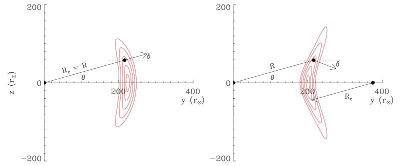
Figure 1: Schematic diagram of MCs at 1 AU in the solar meridianal plane with axes perpendicular to the radial and transverse directions, illustrating the large latitudinal extent and curvature in a uniform (left panel, corresponding to solar maximum) and structured solar wind (right panel, corresponding to solar minimum). Contours denote levels of the initial flux-rope radius. The angles, labeled as $\theta$ and $\delta$, represent the latitude of a virtual spacecraft and the elevation angle of the flux-rope normal. The distance of the spacecraft and radius of flux-rope curvature are marked as $R$ and $R_{c}$, respectively.

From Figure 1, we obtain a simple relationship between the latitude $\theta$ of an observing spacecraft and the normal elevation angle $\delta$ of the flux rope at the spacecraft

$$\delta=\arcsin({R\over R_{c}}\sin\theta).$$ (1)

The radius of curvature, $R_{c}$, is defined such that it is positive when the flux rope is curved away from the Sun (left panel) and negative when curved toward the Sun (right panel). In the left case, $R_{c}=R$, so equation 1 is reduced to $\theta=\delta$. Since MCs are highly flattened as discussed above, the normal would be along the minimum variance direction of the flux-rope magnetic field. The radius of curvature of MCs can be extracted from equation 1 by examining the latitudinal distribution of the normal elevation angles. Lower limits for the transverse size of MCs can be derived from pairs of spacecraft widely separated in latitude. Ulysses, complemented with a near-Earth spacecraft, is particularly useful for this research since it covers latitudes up to 80^∘ [e.g., Hammond et al., 1995; Gosling et al., 1995].

This paper applies the above methodology to give the first direct observational evidence for the large-scale transverse size and curvature of MCs. The data and analysis methods are described in section 2. Sections 3 and 4 give lower limits for the transverse size of MCs and study how they are curved in different solar wind states, respectively. We summarize and discuss the results in section 5.

2 Observations and Data Analysis

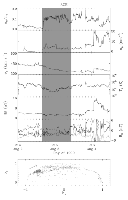
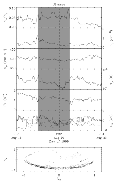
Figure 2: Solar wind plasma and magnetic field parameters measured by ACE (left panel) and Ulysses (right panel) for Case 1 in Table 1. From top to bottom, the panels show the alpha-to-proton density ratio, proton density, bulk speed, proton temperature, magnetic field strength, magnetic components (solid line for $B_{N}$, dotted line for $B_{R}$, dashed line for $B_{T}$), and rotation of the normalized magnetic field vector inside the MC in the maximum variance plane. The shaded region shows the MC. Dashed lines denote the separation of the two flux ropes contained in the MC. Arrows in the bottom panels show the direction of the magnetic field rotation.

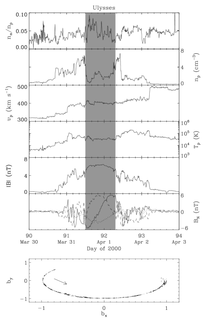
Figure 3: Solar wind plasma and magnetic field parameters for Case 2 in Table 1. Same format as Figure 2.

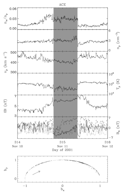
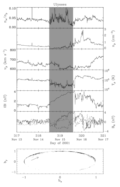
Figure 4: Solar wind plasma and magnetic field parameters for Case 3 in Table 1. Same format as Figure 2.

To give a meaningful measure of the transverse size, we need at least two spacecraft separated as widely as possible in the solar meridianal plane. Launched in 1991, Ulysses explores the solar wind conditions at distances from 1 to 5.4 AU and up to 80^∘ in latitude. Wind and ACE have provided near-Earth measurements (within 7^∘ of the solar equatorial plane) since 1994 and 1998, respectively. We first look for MCs in Ulysses data when it is more than 30^∘ away from the solar equator. If we see the same MC at the near-Earth spacecraft, then its transverse width is at least the spacecraft separation. To determine if the spacecraft observe the same MC, we look at the timing and data similarities (similar transient signatures, the same chirality, etc.), and use a one-dimensional (1-D) MHD model to do data alignment.

We require that the MC axis lie close to the solar equatorial plane. Otherwise, the width we invert is the length of the flux rope other than the transverse size of the cross section; this requirement also minimizes the effect of axial curvature. In addition, our curvature study needs MCs not to be aligned with the radial direction. Wind observations in 1995 - 1997 are used to investigate the MC curvature near solar minimum, while Ulysses as well as the near-Earth spacecraft provides observations from 1999 to 2003 for the curvature study near solar maximum.

2.1 Coordination of Observations via 1-D MHD Modeling

Single-point observations can only sample MCs at a specific distance. As MCs propagate in the solar wind, they may change appreciably. Models are needed to connect observations at different spacecraft. Studies to compare ICME observations at various locations have been performed, using ICME signatures and an MHD simulation to trace their evolution [e.g., Wang et al., 2001; Richardson et al., 2002; Riley et al., 2003]. We follow the same approach and use a 1-D MHD model developed by Wang et al. [2000] to propagate the solar wind from 1 AU to Ulysses. Momentum and energy source terms resulting from the interaction between solar wind ions and interstellar neutrals can be included in this model, but we drop them since they have a negligible effect on the solar wind propagation within Ulysses’ distance. All physical quantities at the inner boundary (1 AU) are set to the average near-Earth solar wind conditions; the MHD equations are then solved by a piecewise parabolic scheme to give a steady state solar wind solution. Observations at 1 AU (typically 60 days long) containing the ICME data are introduced into the model as perturbations. The numerical calculation stops when the perturbation has traveled to Ulysses. The model output is compared with Ulysses observations. Note that the 1-D model assumes spherical symmetry, so we do not expect the model output to exactly match the Ulysses data. Nevertheless, large stream structures should be similar and allow us to align these data sets.

2.2 Minimum Variance Analysis

The axis orientation of MCs is needed to specify their global structure. Minimum variance analysis (MVA) of the measured magnetic field yields useful principle axes [e.g., Sonnerup and Cahill, 1967; Sonnerup and Scheible, 1998]. A normal direction, $\hat{\bf n}$, can be identified by minimizing the deviation of the field component ${\bf B}^{m}\cdot\hat{\bf n}$ from $\langle{\bf B}\rangle\cdot\hat{\bf n}$ for a series of measurements of $m=1,\ldots,N$

$$\sigma^{2}={1\over N}\sum_{m=1}^{N}|({\bf B}^{m}-\langle{\bf B}\rangle)\cdot\hat{\bf n}|^{2},$$ (2)

where $\langle{\bf B}\rangle$ is the average magnetic field vector. Optimizing the above equation under the constraint of $|\hat{\bf n}|^{2}=1$ results in the eigenvalue problem of the covariance matrix of the magnetic field

$$M_{\mu\nu}=\langle B_{\mu}B_{\nu}\rangle-\langle B_{\mu}\rangle\langle B_{\mu}\rangle,$$ (3)

where $\mu,\nu$ indicate the field components in Cartesian coordinates. Eigenvectors of the matrix, $\hat{\bf x}^{\star}$, $\hat{\bf y}^{\star}$, $\hat{\bf z}^{\star}$, corresponding to the eigenvalues in order of decreasing magnitude, denote the the maximum, intermediate and minimum variance directions. The normal of an elongated flux rope should be along the minimum variance direction (see Figure 1); the maximum variance would occur azimuthally since the azimuthal component changes its sign across the flux rope; the intermediate variance direction is identified as the axis orientation due to the non-uniform distribution of the axial field over the flux-rope cross section. The MVA method also gives the chirality of the flux-rope fields as shown in the bottom panels of Figures 2, 3 and 4.

Angular error estimates of the directions can be written as [Sonnerup and Scheible, 1998]

$$\Delta\varphi_{ij}=\sqrt{{\lambda_{z}(\lambda_{i}+\lambda_{j}-\lambda_{z})\over(N-1)(\lambda_{i}-\lambda_{j})^{2}}}$$ (4)

for $i,j\in\{\hat{\bf x}^{\star},\hat{\bf y}^{\star},\hat{\bf z}^{\star}\}$ and $i\neq j$, where $\lambda_{i}$ denotes the eigenvalue of the variance matrix, and $\Delta\varphi_{ij}$ represents the angular uncertainty of eigenvector $i$ with respect to eigenvector $j$. The uncertainty of the normal elevation angle $\delta$ is

$$\Delta\varphi_{z}=\sqrt{(\Delta\varphi_{zx})^{2}+(\Delta\varphi_{zy})^{2}},$$ (5)

where we assume that the errors are independent.

2.3 Grad-Shafranov Technique

Table 1: Estimated parameters of MCs at ACEa  and Ulyssesa

No.	Year	CME Onsetb	Start	End	$R$c	$\theta$c	$\phi$c	$\Theta$d	$\Phi$d	Chirality
					(AU)	(∘)	(∘)	(∘)	(∘)
1	1999	Jul 29, 05:43	Aug 2, 15:36	Aug 3, 10:34	1	5.9	234.3	$-$42.4 ($-$48.8)	251.2 (261.5)	L
	1999	-	Aug 19, 00:00	Aug 20, 12:00	4.7	$-$32.3	87.4	$-$7.1 ($-$11.3)	283.9 (261.9)	L
2	2000	Mar 14, 10:08	Mar 19, 03:22	Mar 19, 12:43	1	$-$7.1	103.0	24.3 (29.2)	51.4 (95.8)	R
	2000	-	Mar 31, 12:00	Apr 1, 07:12	3.7	$-$50.1	93.1	19.1 (13.6)	112.2 (90.0)	R
3	2001	Nov 6, 16:39	Nov 10, 19:12	Nov 11, 07:55	1	3.3	333.0	$-$37.8 ($-$16.5)	151.1 (121.9)	L
	2001	-	Nov 14, 12:00	Nov 15, 14:24	2.3	75.4	39.5	$-$16.6 ($-$15.4)	104.7 (103.4)	L
PRe	1999	Feb 15, -f	Feb 18, 13:55	Feb 19, 11:02	1	$-$7.0	74.0	0.4 ($-$30.1)	277.1 (284.7)	L
	1999	-	Mar 3, 21:36	Mar 5, 21:36	5.1	$-$22.3	85.2	$-$38.0 ($-$35.3)	269.3 (265.2)	L

aCorresponding to the first and second lines for each case, respectively. bObtained by extrapolating the quadratic fit of the CME’s height-time curve to the solar surface. cHeliographic inertial distance, latitude and longitude of the spacecraft. dAxis elevation angle with respect to the solar equatorial plane and azimuthal angle in RTN coordinates, estimated from MVA (outside parentheses) and the GS technique (inside parentheses). eThe case studied by Riley et al. [2003]. fNo CMEs observed at the Sun on 1999 February 15.

Initially designed for the study of the terrestrial magnetopause [e.g., Hau and Sonnerup], the GS technique can be applied to flux-rope reconstruction [e.g., Hu and Sonnerup, 2002]. It assumes an approximate deHoffmann-Teller (HT) frame in which the electric field vanishes everywhere. Structures in such a frame obey MHD equilibrium, ${\bf j}\times{\bf B}-\nabla p=0$, which can be reduced to the so-called GS equation [e.g., Sturrock, 1994]

$${\partial^{2}A\over\partial x^{2}}+{\partial^{2}A\over\partial y^{2}}=-\mu_{0}{d\over dA}(p+{B_{z}^{2}\over 2\mu_{0}})$$ (6)

by assuming a translational symmetry along the flux rope (i.e., $\partial\over\partial z$=0). The vector potential is defined as ${\bf A}=A(x,y)\hat{\bf z}$, through which the magnetic field is given by ${\bf B}=({\partial A\over\partial y},-{\partial A\over\partial x},B_{z})$.

The key idea in reconstructing the flux rope is that the thermal pressure $p$ and the axial field $B_{z}$ are functions of $A$ alone. The flux-rope orientation is determined by the single-valued behavior of the transverse pressure $p_{t}=p+B_{z}^{2}/2\mu_{0}$ over the vector potential $A$, which essentially requires that the same field line be crossed twice by an observing spacecraft. Once the invariant $z$ axis is acquired, the right-hand side of equation 6 can be derived from the differentiation of the best fit of $p_{t}$ versus $A$. This best fit is assumed to hold over the entire flux-rope cross section. Away from the observation baseline, the vector potential $A$ is calculated based on its second order Taylor expansion with respect to $y$. Since the integration is intrinsically a Cauchy problem, numerical singularities are generated after a certain number of steps. As a result, the transverse size is generally limited to half of the width along the observation line in the integration domain. Detailed procedures can be found in Hau and Sonnerup [1999] and Hu and Sonnerup [2002]. Here we only use this approach to determine the axis orientation of MCs and make a comparison with MVA.

3 Lower Limits of the Transverse Extent

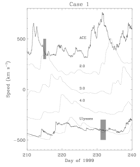
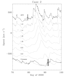
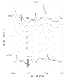
Figure 5: Evolution of solar wind speed from ACE to Ulysses for the three cases in Table 1 via the 1-D MHD model. The upper and lower solid lines show the solar wind speeds observed at ACE and Ulysses, while the dotted lines indicate the speed profiles predicted by the model at distances (in AU) marked by the numbers. Shaded regions represent the period where the MC was observed at ACE and Ulysses. Each speed curve is decreased by 200 km s^-1 (left panel) and 160 km s^-1 (middle and right panels) with respect to the previous one so that the individual line shapes can be easily deciphered. For Case 3 (right panel), the profile at Ulysses is shifted downward by 1360 km s^-1 from the observed speed, while the model output at 2.3 AU is shifted by 1040 km s^-1 to line up with the Ulysses data; the model output at Ulysses underestimates the observed speed by 320 km s^-1.

Application of the criteria and restrictions given in section 2 yields three MCs observed at both ACE and Ulysses with a latitudinal separation larger than $30^{\circ}$. Table 1 lists the times, locations, estimated axis orientations and chiralities for ACE and Ulysses observations, respectively. The distance $R$, latitude $\theta$ and longitude $\phi$ of the spacecraft are given in the heliographic inertial frame. The MC denoted as PR in the table was shown to be observed at both the spacecraft by Riley et al. [2003] through a qualitative comparison between data and an MHD model output; the two spacecraft were separated by $15^{\circ}$ in latitude. Table 1 also gives the CMEs observed at the Sun (adopted from http://cdaw.gsfc.nasa.gov/CME_-list) that best match the occurrence time calculated from the MC’s transit speed at 1 AU. Applications of the MVA method to the normalized magnetic field measurements and the GS technique to the plasma and magnetic field observations within the MCs give the axis orientation, in terms of the elevation ($\Theta$) and azimuthal ($\Phi$) angles. The axis azimuthal angle is given in RTN coordinates (in which ${\bf R}$ points from the Sun to the spacecraft, ${\bf T}$ is parallel to the solar equatorial plane and points to the planet motion direction, and ${\bf N}$ completes the right-handed triad), which allows us to see if the axis is perpendicular to the radial direction (i.e., close to 90^∘ or 270^∘). The magnetic field and velocity vectors inside the MCs are rotated into the heliographic inertial frame in order to have an axis elevation angle with respect to the solar equatorial plane. The estimates of the axis orientation from the MVA and GS methods roughly agree. The MCs generally lie close to the solar equator and perpendicular to the radial direction. The MC travel time from ACE to Ulysses is consistent with the observed speeds. They also have the same chirality as listed in Table 1.

Figure 2 shows the plasma and magnetic field measurements for Case 1 in Table 1 at ACE and Ulysses separated by 38^∘ in latitude. Its boundaries are mainly determined from the low proton temperature combined with enhanced helium abundance. The helium enhancement has been shown to be an effective tool to trace ICMEs from 1 AU to Ulysses and Voyager 2 [e.g., Paularena et al., 2001; Richardson et al., 2002]. The MVA of the magnetic field measurements inside the MC at ACE and Ulysses gives an eigenvalue ratio $\lambda_{x}:\lambda_{y}:\lambda_{z}$ of $6:1:0.8$ and $3.2:1:0.2$, respectively. The MC has a relatively large axis elevation angle ($>40^{\circ}$) at ACE, probably due to the small separation between $\lambda_{y}$ and $\lambda_{z}$; the axis orientation is close to the solar equator at Ulysses. The bottom panels of Figure 2 display the normalized magnetic field inside the MC projected onto the maximum variance plane. The majority of the data show a coherent rotation of about $180^{\circ}$; both the rotations indicate a left-handed chirality of the magnetic configuration. Interestingly, the GS reconstruction shows that this case contains two nested flux ropes in both ACE and Ulysses measurements. Marked as a dashed line in Figure 2, the separation of the two flux ropes in both ACE and Ulysses observations appears as a discontinuity in the proton density (second panels) and magnetic field components (sixth panels). A shock wave, indicated by simultaneous sharp increases in the proton density, speed, temperature and magnetic field strength, follows the MC at ACE and Ulysses (not shown in the Ulysses data).

Figure 3 displays the data for Case 2 at ACE and Ulysses separated by 43^∘ in latitude. ACE and Ulysses are roughly aligned in longitude for this case. The boundaries are determined from the rotation of the magnetic field together with the low proton temperature. This event is also associated with a small bump in the helium/proton density ratio. The eigenvalue ratio $\lambda_{x}:\lambda_{y}:\lambda_{z}$ determined from the MVA is $2.5:1:0.2$ and $3.2:1:0.02$ for ACE and Ulysses observations, respectively. It drives a forward shock at Ulysses which may also be seen at ACE, but data gaps at ACE make it difficult to locate the shock. Again, the normalized magnetic field data inside the MC at ACE and Ulysses show a right-handed rotation in the maximum variance plane.

Figure 4 shows the data for Case 3 which has the largest separation (72^∘) in latitude between ACE and Ulysses. Depressed proton temperature and magnetic field rotation combined with enhanced helium abundance are used to determine the boundaries. The velocity and magnetic field fluctuations are strongly anti-correlated outside the MC both at ACE and Ulysses, which indicates the presence of Alfvén waves; this wave activity also occurs within the MC but at a reduced fluctuation level. The eigenvalue ratio $\lambda_{x}:\lambda_{y}:\lambda_{z}$ from the MVA is $6.8:1:0.3$ for ACE measurements and $3.4:1:0.1$ for Ulysses observations. Smooth rotations of about 180^∘ in the magnetic field (bottom panels) indicate a left-handed chirality.

We propagate the ACE data to Ulysses using the 1-D MHD model described in section 2. Figure 5 shows the velocity profiles observed at ACE and Ulysses (solid lines), and the model profiles at certain distances (dotted lines) for the three cases. In all of these cases, larger streams at 1 AU persist to Ulysses as clearly shown by the traces and model-data comparison at Ulysses, while smaller ones smooth out. For Cases 1 and 2 (left and middle panels), the model outputs at Ulysses agree qualitatively well with the observed speed profiles. Note that the model-predicted and observed speeds were not shifted to produce this agreement. For Case 3 (right panel), the model predicts a slower solar wind than observed at Ulysses, which is reasonable given the large latitudinal separation (72^∘) between ACE and Ulysses and possible differences in the ambient solar wind. Based on the good stream alignment and data similarities shown in Figures 2, 3 and 4, we conclude that the two spacecraft see the same events.

The MCs listed in Table 1 offer observational evidence for the large transverse size of ICMEs. In order to quantify the transverse size, we examine the latitudinal separation between ACE and Ulysses for these MCs. The latitudinal separation ($\Delta\theta$) serves as a measure of the transverse size, $S_{t}$, expressed as

$$S_{t}=R\Delta\theta,$$ (7)

where $R$ is the heliocentric distance of the MCs at Ulysses. This equation explicitly assumes that the latitudinal extent of the MCs is constant during their propagation through the solar wind. The results for the present MCs are plotted in Figure 6. The transverse size given by the above equation is much larger than the MCs’ radial width obtained from their average speed multiplied by the time duration. As can seen from Figure 6, the largest aspect ratio is $15.6:1$. The PR event has a ratio of $2.6:1$ since $\Delta\theta$ is only 15.3^∘ for this case. Figure 6 reveals that the MCs have a cross section greatly elongated in the latitudinal direction.

The large transverse size can also be inferred from the shock standoff distance $d$ ahead of fast MCs written as [Russell and Mulligan, 2002]

$${d\over L}=0.41{(\gamma-1)M^{2}+2\over(\gamma+1)(M^{2}-1)},$$

where $\gamma={5\over 3}$, $M$ is the Mach number of the preceding shock, and $L$ is the characteristic scale of MCs, presumably a measure of $S_{t}$. From the superposed epoch data of 18 near-Earth MCs with preceding shocks in Liu et al. [2006b, Figure 8], we have $M=3.4$ and $d=0.17$ AU on average. Substitution of these values into the above equation gives $L=1.2$ AU, which corresponds to a latitudinal extent of $\sim$ 69^∘ obtained from equation 7. Consistent with our direct evidence, the transverse size of MCs (or ICMEs in general) could be very large.

4 Curvature of Magnetic Clouds

A direct consequence of the large transverse size is that MCs encounter different solar wind flows in the meridianal plane. MCs can thus be highly distorted depending on the ambient solar wind conditions. The simplified scenario described in section 1 indicates that MCs should be ideally concave outward at solar minimum and convex outward during solar maximum. This curvature effect results in an inverse correlation between $\delta$ and $\theta$ at solar minimum and a positive correlation near solar maximum as shown by equation 1. Note, however, that this is a greatly simplified picture. In reality, the shape of MCs will be determined by the speed at which they travel with respect to the background solar wind, ambient magnetic fields, the presence of other ICMEs or obstacles nearby, and other features that are beyond the scope of this paper.

As discussed in section 2, the distortion effect by solar wind flows would be most prominent if MCs have axes close to the solar equator and perpendicular to the radial direction. In order to have enough events for our curvature analysis, we include all the MCs whose axes lie within 30^∘ of the solar equatorial plane and more than 30^∘ away from the radial direction.

4.1 MCs in a Structured Solar Wind

Close to solar minimum, the solar wind is well ordered with fast wind originating from polar coronal holes and slow wind near the solar equatorial plane. Wind observations from 1995 - 1997 are used to assess the distortion effect of the latitudinal flow gradient on MCs. Figure 7 shows the normal elevation angles for the 14 events observed at Wind. The error bars are obtained from equation 5. An inverse correlation is observed between $\delta$ and $\theta$, except for three events. The MCs are expected to be concave outward during solar minimum, which is largely observed, made evident by the inverse relationship plotted as a solid line. The three events where $\delta$ and $\theta$ have the same sign indicate a convex outward curvature, contrary to the solar minimum prediction. A closer look at the 1997 May 15 event reveals an increasing speed profile indicative of a high-speed stream interacting with the sunward edge of the MC. As a result, the MC is bent to be convex outward. Note that the simplified picture described in section 1 assumes a minimum solar wind speed at the solar equator. It is conceivable that $\delta$ and $\theta$ may have the same sign if the minimum speed shifts away from the zero latitude. Although the breakdown of the assumption is a possible explanation for the other two exceptions, this effect may be negligible since most of the events in Figure 7 have the inverse correlation. The best fit to the data that show the inverse correlation, obtained with a least squares analysis of equation 1, gives a radius of curvature of $-0.3$ AU. Compared with the convex-outward representation (dashed line), the data clearly show the trend pictured by the right panel of Figure 1.

4.2 MCs in a Uniform-Speed Solar Wind

At solar maximum, the solar wind speed tends to be more uniform over heliographic latitude. We use Ulysses observations between 1999 and 2003 to quantify the curvature effect of solar wind spherical expansion on MCs. Our prescription yields 13 events shown in Figure 8. In a uniform solar wind the MCs would have a radius of curvature equal to their distance from the Sun, which results in a proportional relationship, i.e., $\delta=\theta$ from equation 1. Only two events do not have a positive correlation. More specifically, $\delta$ and $\theta$ have opposite signs for the two events. They are the first and last ones in the time series of the MCs; as indicated by the dates, they may not truly come from the solar maximum environment. The data nearby the $\delta=\theta$ curve (dashed line) manifest a convex-outward structure at solar maximum as illustrated by the left panel of Figure 1.

5 Summary and Discussion

We have investigated the transverse size and curvature of the MC cross section, based on ACE, Wind and Ulysses observations. The results provide compelling evidence that MCs are highly stretched in the latitudinal direction and curved in a fashion depending on the background solar wind.

Three MCs, whose axes are close to the solar equator and roughly perpendicular to the radial direction, are shown to pass ACE and Ulysses (widely separated in latitude) successively. The MVA method combined with the GS reconstruction technique is used to determine the axis orientation and the observations at ACE and Ulysses are linked using a 1-D MHD model. The latitudinal separation between ACE and Ulysses gives a lower limit to the MCs’ transverse size. Varying from 40^∘ to 70^∘, it reveals that the transverse size can be very large. The flattened cross section is a natural result of a flux rope subtending a constant angle as it propagates from the Sun through the heliosphere (see Figure 1).

The radius of curvature is obtained from a simple relationship between the MC normal elevation angle and the latitude of an observing spacecraft. The curvature of MCs in the solar wind with a latitudinal speed gradient at solar minimum differs from that in the uniform-speed solar wind near solar maximum. At solar minimum, MCs are bent concave-outward by the structured solar wind with a radius of curvature of about 0.3 AU; at solar maximum, they tend to be convex outward with the radius of curvature proportional to their heliographic distance. The distortion of MCs, resulting from the interaction with the ambient solar wind, is mainly a kinematic effect since magnetic forces are dominated by the flow momentum [Riley and Crooker, 2004].

Improvement of our knowledge of the global structure of MCs (or generic ICMEs) is of critical importance for heliosphere physics and space weather prediction. Proper estimates of the magnetic flux and helicity of ICMEs require knowledge of the structure to quantify their connection with the coronal origin and to assess the modulation of heliospheric flux by CMEs. The large transverse size and curvature can alter the global configuration of the interplanetary magnetic field as ICMEs sweep through the heliosphere. Numerical simulations show that the ambient magnetic field extending from the Sun to high latitudes may bend poleward to warp around the flattened flux rope [e.g., Manchester et al., 2004], as initially proposed by Gosling and McComas [1987] and McComas et al. [1988]. The field line draping leads to favorable conditions for the formation of plasma depletion layers and mirror mode instabilities in the sheath region of fast ICMEs [Liu et al., 2006b]. A magnetic field bent southward would also allow for strong coupling between the solar wind and the magnetosphere via field line merging [Dungey, 1961]. The curvature of ICMEs could modify the shape of preceding shock fronts, affecting plasma flows and particle acceleration at the shocks.

Figure 6: Latitudinal separation between ACE and Ulysses for the MCs listed in Table 1 as a function of Ulysses’ heliocentric distance. The horizontal bars show the radial width of the MCs, and the vertical bars indicate the lower limit of the transverse size (converted to a length scale). Text depicts the corresponding ratio of the two scales.

Figure 7: Elevation angles of the MC normal from the solar equatorial plane as a function of Wind’s heliographic latitude. Circles with a nearby date indicate events that do not have an inverse correlation. The solid line represents the best fit of the data that obey the relationship using equation 1. The radius of curvature resulting from the fit is given by the text in the figure. The dashed line shows what would be expected if the MCs were convex outward with a radius of curvature of 1 AU.

Figure 8: Elevation angles of the MC normal from the solar equatorial plane as a function of Ulysses’ heliographic latitude. Circles with a nearby date indicates events that do not have a positive correlation. The dashed line represents $\delta=\theta$.

How general ICMEs are distorted remains unaddressed. Since their magnetic field is not well organized, the difficulty resides in how to best estimate their axis orientation. Future Stereo observations will provide perspectives for their geometry and also quantitatively test our results for MCs.