Theory of Earthquake Recurrence Times

A. Saichev¹ and D. Sornette^2,3

¹ Mathematical Department, Nizhny Novgorod State University

Gagarin prosp. 23, Nizhny Novgorod, 603950, Russia

² D-MTEC, ETH Zurich, CH-8032 Zürich, Switzerland (email: dsornette@ethz.ch)

³ LPMC, CNRS UMR6622 and Université des Sciences, Parc Valrose, 06108 Nice Cedex 2, France

Abstract: The statistics of recurrence times in broad areas have been reported to obey universal scaling laws, both for single homogeneous regions (Corral, 2003) and when averaged over multiple regions (Bak et al.,2002). These unified scaling laws are characterized by intermediate power law asymptotics. On the other hand, Molchan (2005) has presented a mathematical proof that, if such a universal law exists, it is necessarily an exponential, in obvious contradiction with the data. First, we generalize Molchan’s argument to show that an approximate unified law can be found which is compatible with the empirical observations when incorporating the impact of the Omori law of earthquake triggering. We then develop the full theory of the statistics of inter-event times in the framework of the ETAS model of triggered seismicity and show that the empirical observations can be fully explained. Our theoretical expression fits well the empirical statistics over the whole range of recurrence times, accounting for different regimes by using only the physics of triggering quantified by Omori’s law. The description of the statistics of recurrence times over multiple regions requires an additional subtle statistical derivation that maps the fractal geometry of earthquake epicenters onto the distribution of the average seismic rates in multiple regions. This yields a prediction in excellent agreement with the empirical data for reasonable values of the fractal dimension $d\approx 1.8$, the average clustering ratio $n\approx 0.9$, and the productivity exponent $\alpha\approx 0.9$ times the $b$-value of the Gutenberg-Richter law. Our predictions are remarkably robust with respect to the magnitude threshold used to select observable events. These results extend previous works which have shown that much of the empirical phenomenology of seismicity can be explained by carefully taking into account the physics of triggering between earthquakes.

1 Introduction

The concept of “recurrence time” (also called recurrence interval, inter-event time or return time) is widely used for hazard assessment in seismology. The average recurrence time of an earthquake is usually defined as the number of years between occurrences of an earthquake of a given magnitude in a particular area. Once chosen a probabilistic model for the distribution of recurrence times (often a Poisson distribution in earlier implementations, evolving progressively to more realistic distributions), an estimation of the probability for damaging earthquakes in a given area over a specific time horizon can be derived. For instance, the Working Group on Califonia Earthquake Probabilities (2003) assessed a 0.62 probability of a major damaging earthquake striking the greater San Francisco Bay Region over the following 30 years (2002-2031). Such calculations are based on classifications of known active faults and on assumptions about the organization of seismicity on these faults, guided by geological, paleoseismic (see for instance Sieh, 1981), geodetic evidence (Global Earthquake Satellite System, 2003) as well as earthquake patterns extracted from recent seismic catalogs. Starting with the simple assumption that faults are independent and carry their own characteristic earthquake (Schwartz and Coppersmith, 1984), seismologists and other scientists working on seismic hazards are realizing that more complex models are needed to take into account the interaction, coupling and competition between faults (Lee et al., 1999) which translates into a rich phenomenology in the space-time-magnitude organization of earthquakes.

A new view is now emerging that recurrence times should be considered for broad areas, rather than for individual faults, and could provide important insights in the physical mechanisms of earthquakes. For instance, Wyss et al. (2000) have proposed to relate an indirect measurement of local recurrence times within faults to geometrical asperities and stress field, thus significantly broadening the standard notion of return time. Inspired by the scaling approach developed in the physics of critical phenomena (Sornette, 2004), Kossobokov and Mazhkenov (1988), Bak et al. (2002) and Christensen et al. (2002) have proposed a unified scaling law combining the Gutenberg-Richter law, the Omori law and the fractal distribution of epicenters to describe the distributions of inter-event times between successive earthquakes in a hierarchy of spatial domain sizes and magnitudes in Southern California. Corral (2003, 2004a,b, 2005a) has refined and extended these analyses to many different regions of the world and has proposed the existence of a universal scaling law for the probability density function (PDF) $H(\tau)$ of recurrence times (or inter-event times) $\tau$ between earthquakes in a given region $S$:

$$H(\tau)\simeq\lambda f(\lambda\tau)~{}.$$ (1)

The remarkable proposition is that the function $f(x)$, which exhibit different power law regimes with cross-overs, is found almost the same for many different seismic regions, suggesting universality. The specificity of a given region seems to be captured solely by the average rate $\lambda$ of observable events in that region, which fixes the only relevant characteristic time $1/\lambda$ for the recurrence times.

The interpretation proposed by Bak et al. (2002), Christensen et al. (2002) and Corral (2003, 2004a,b, 2005a) is that the scaling law (1) reveals a complex spatio-temporal organization of seismicity, which can be viewed as an intermittent flow of energy released within a self-organized (critical?) system, for which concepts and tools from the theory of critical phenomena can be applied (Corral, 2005b). This view has been challenged by Lindman et al. (2005) who stressed several methodological caveats (see Corral and Christensen (2006) for a reply). Livina et al. (2005) have additionally noticed that the marginal (or mono-variate) PDF of inter-event times gives only a partial description of the time sequence of earthquakes in a given region, as it is found to be a function of preceding inter-event times. There is thus a memory between successive earthquakes which influences the distribution of the inter-event times, a conclusion which is well-known to most seismologists.

It is fair to state that there is at present no theoretical understanding of these empirical results and in particular of expression (1). The situation becomes even more interesting with the recent mathematical demonstration by Molchan (2005) that, under very weak and general conditions, the only possible form for $f(x)$, if universality holds, is the exponential function, in strong disagreement with the observations reported by Bak et al. (2002) and Corral (2003, 2004a,b, 2005a). In addition, from a re-analysis of the seismicity of Southern California, Molchan and Kronrod (2005) have shown that the unified scaling law (1) is incompatible with multifractality which seems to offer a better description of the data.

Here, our purpose is to show how all the above can be simply understood and reconciled from the standard known statistical laws of seismicity:

• (i) the Gutenberg-Richter distribution $\sim 1/E^{1+\beta}$ (with $\beta\approx(2/3)b\approx 2/3$) of earthquake energies $E$ (Knopoff et al., 1982);

• (ii) the Omori law $\sim 1/t^{p}$ (with $p\approx 1$ for large earthquakes) of the rate of aftershocks as a function of time $t$ since a mainshock (Utsu et al., 1995);

• (iii) the productivity law $\sim E^{a}$ (with $a\approx 2/3$) giving the number of earthquakes triggered by an event of energy $E$ (Helmstetter et al., 2005);

• (iv) the fractal (and even probably multifractal (Ouillon et al., 1996)) structure of fault networks (Davy et al, 1990) and of the set of earthquake epicenters (Kagan and Knopoff, 1980).

The question we address can be summarized as follows: are the statistics on inter-event times described in (Bak et al., 2002; Corral, 2003, 2004a,b, 2005a; Livina et al., 2005) really new in the sense that they reveal some information which is not contained in the above laws (i-iv), as claimed by these authors? Or can they be derived from the known statistical properties of seismicity, so that they are only different ways of presenting the same information?

In order to address this question, we use the simplest possible model which combines these four laws, framed as a stochastic point process of past earthquakes triggering future earthquakes: the Omori law (ii) is taken to describe the conditional rate of activation of new earthquakes, given all past earthquakes; the Gutenberg-Richter law (i) describes the distribution according to which the magnitude of a new earthquake is independently determined; the productivity law (iii) gives the weight of the contribution of a given past earthquake in the production of new earthquakes. In order to take into account the fractal geometry of earthquake catalogs, the new earthquakes can be positioned on a fractal geometry. The elements (i-iii) actually constitute the basic building block of the benchmark model of seismicity, known as the Epidemic-Type Aftershock Sequence (ETAS) model of triggered seismicity (Ogata, 1988; Kagan and Knopoff, 1981), whose main statistical properties are reviewed in (Helmstetter and Sornette, 2002). Various versions have been or are currently applied by different groups to describe observed and forecast future seismicity (Console et al., 2002; 2003a,b; 2006; Console and Murru, 2001; Gerstenberger et al., 2005; Reasenberg, P. A. and Jones, 1989; 1994; Steacy et al., 2005).

The common characteristics of this class of models is to treat all earthquakes on the same footing such that one does not assume any distinction between foreshocks, mainshocks and aftershocks: each earthquake is considered to be capable of triggering other earthquakes according to the three basic laws (i-iii) mentioned above. This hypothesis is based on the realization that there are no observable differences between foreshocks, mainshocks and aftershocks (Jones et al., 1999; Helmstetter and Sornette, 2003a; Helmstetter et al., 2003), notwithstanding their usual classification based in retrospect analysis of realized seismic sequences: Earthquakes preceding the mainshock are called foreshocks and earthquakes following the mainshock are called aftershocks but no physical differences between these earthquakes are known. For instance, a mainshock (classified as the largest event in a given space-time window) may be re-classified as a foreshock if a larger event later follows it; and what would have been an aftershock becomes a mainshock if larger than all its preceding earthquakes.

In this paper, we use specifically the ETAS model in the version proposed by Ogata (1988). The ETAS model assumes that earthquakes magnitudes are mutually statistically independent and drawn from the Gutenberg-Richter (GR) probability $Q(m)$. The GR law gives the probability that magnitudes of triggered events are larger than a given level $m$ (the relationship between magnitude $m$ and energy is $m\propto(2/3)\ln_{10}E$). We shall use the GR law in the form

$$Q(m_{2})=Q(m_{1})10^{-b(m_{2}-m_{1})}~{},$$ (2)

which emphasizes its scale invariance property. Here $b\simeq 1$ and $m_{1}$, $m_{2}$ are arbitrary magnitudes. We parameterize the (bare) Omori law (Sornette and Sornette, 1999; Helmstetter and Sornette, 2002) for the rate of triggered events of first-generation from a given earthquake as

$$\Phi(t)={\theta c^{\theta}\over(c+t)^{1+\theta}}$$ (3)

with $\theta\gtrsim 0$. One may interpret $\Phi(t)$ as the PDF of random times of independently occurring first-generation aftershocks, triggered by some mainshock which happened at the origin $t=0$. The last ingredient is the productivity law, which we write in the following convenient form for further analysis,

$$\rho(m)=\kappa~{}10^{\alpha(m-m_{0})}~{},$$ (4)

where the factor $\kappa$ will be related below to physically observable quantities such as the average branching ratio $n$ (which is the average number of triggered earthquakes of first generation per triggering event). The magnitude $m_{0}$ is a cut-off introduced to regularize the theory (Helmstetter and Sornette, 2002). It can be interpreted as the smallest possible magnitude for earthquakes to be able to trigger other earthquakes (Sornette and Werner, 2005a). Several authors have shown that the ETAS model provides a good description of many of the regularities of seismicity (Console et al., 2002; 2003a,b; 2006; Console and Murru, 2001; Helmstetter and Sornette, 2003a,b; Helmstetter et al., 2005; Gerstenberger et al., 2005; Ogata, 1988; 2005; Ogata and Zhuang, 2006; Reasenberg, P. A. and Jones, 1989; 1994; Saichev and Sornette, 2005; 2006a; Steacy et al., 2005; Zhuang et al., 2002; 2004; 2005).

Our main result is that, according to Occam’s razor, the previously mentioned results on universal scaling laws of inter-event times do not reveal more information than what is already captured by the well-known laws (i-iii) of seismicity (Gutenberg-Richter, Omori, essentially), together with the assumption that all earthquakes are similar (no distinction between foreshocks, mainshocks and aftershocks), which is the key ingredient of the ETAS model. Our theory is able to account quantitatively for the empirical power laws found by Bak et al. and Corral, showing that they result from subtle cross-overs rather than being genuine asymptotic scaling laws. We also show that universality does not strictly hold.

The organization of the paper is the following. In section 2, we discuss in detail Molchan’s derivation (Molchan, 2005) that, if the scaling law (1) holds true, then it should be exponential in the sense that $f(x)=e^{-x}$. We extend Molchan’s argument by developing a simple semi-quantitative theory, showing that the presence of the Omori law destroys the self-similarity of the PDF of recurrence times. Nevertheless, if the exponent of the Omori law (3) is close to $1$, i.e., $\theta\ll 1$, then, the PDF of recurrence times approximately obeys a non-exponential scaling law which can fit well the empirical data. Section 3 extends further the discussion of section  2 by proposing simplified models of aftershock triggering process, in the goal of demonstrating the direct relation between the Omori law and the corresponding scaling law for the PDF of the recurrence times for an arbitrary region. These discussions allow us to stress the generality of the curve that we propose to the disagreement between Molchan’s result and empirical data. They also prepare us to understand better the full derivation using the technology of generating probability functions (GPF) applied to the ETAS model. In section 4, we analyze the ETAS model of triggered seismicity with the formalism of GPF and establish the main general results useful for the following. As a check for the formalism, we obtain the statistical description for the number of observable events which occur within a given region and during the time window $[t,t+\tau]$. Section 5 exploit the general results of section 4 to obtain predictions on the PDF of recurrence times between observable events in a single homogeneous region characterized by a well-defined average seismic rate. A short account of some of these results is presented in (Saichev and Sornette, 2006c). Section 6 combines the previous results on single regions to obtain predictions of the PDF of inter-event times between earthquakes averaged over many different regions. In a first part, we construct different ad hoc models of the distribution of the average seismic rates of different regions. In a second part, we propose a procedure converting the fractal geometry of epicenters into a specific distribution of the average seismic rates of different regions. The knowledge of this distribution allows us to compute the PDF of inter-event times averaged over many regions which is compared with Bak et al. (2002)’s and Corral (2004a)’s empirical analyses. We find a very good agreement between our prediction and the empirical PDF of inter-event times.

2 Generalized Molchan’s relation

We start by addressing the puzzle raised by the demonstration by Molchan (2005) based on a probabilistic reasoning that, under very weak and general conditions, the only possible form for $f(x)$ in (1), if universality holds, is the exponential function, in contradiction with the strongly non-exponential form of the reported seemingly universal unified PDF (1) for inter-event times. Here, we briefly reproduce Molchan’s argumentation and then generalize it to show that the presence of the Omori law, while destroying the exact unified law, gives nevertheless an approximate unified law fitting rather precisely the real data.

Let $P(\tau)$ be the probability that there are no observable events during the time interval $[t,t+\tau]$ within some region $S$. Let us call $\lambda$ the average rate of observable events within the region $S$. Let us assume the existence of a unified law

$$P(\tau)=\varphi(\lambda\tau)~{},$$ (5)

valid for any region. In expression (5), $\varphi(x)$ is the universal scaling function, which is assumed to be the same for all regions. Following Molchan’s argument, if an unified law (5) holds true for any region, then it should be valid for the region made of the union of two disjoint regions characterized respectively by the rates $\lambda_{1}$ and $\lambda_{2}$. If the triggering processes of earthquake in those two regions are statistically independent, then the following functional equation should be true

$$\varphi((\lambda_{1}+\lambda_{2})\tau)=\varphi(\lambda_{1}\tau)\varphi(\lambda_{2}\tau)~{}.$$ (6)

Posing $\psi(x)=\ln\varphi(x)$, the equation (6) is equivalent to

$$\psi(x)=\psi\left({\lambda_{1}\over\lambda_{1}+\lambda_{2}}x\right)+\psi\left({\lambda_{2}\over\lambda_{1}+\lambda_{2}}x\right)~{}.$$ (7)

It is well-known that the solution of equation (7) defines the class of linear funtions $\psi(x)=-ax$ for arbitrary $a$’s, leading to the exponential form

$$\varphi(x)=e^{-ax}~{}.$$ (8)

For the PDF (5), there is a normalization condition that allows us to fix the constant $a$. We need first to recall a few general results of the theory of point processes (Daley and Vere-Jones, 1988) Let the random times

$$\dots t_{-1},t_{0},t_{1},\dots t_{k}\dots\qquad t_{k+1}>t_{k}>t_{k-1}\dots$$ (9)

form a stationary point process with an average rate equal to $\lambda$. Then, the PDF $H(\tau)$ of the inter-event times $t_{k+1}-t_{k}$ can be obtained from the following relation

$$H(\tau)={1\over\lambda}{d^{2}P(\tau)\over d\tau^{2}}~{},$$ (10)

where $P(\tau)$ is the already mentioned probability of absence of events within the interval $[t,t+\tau]$. The normalization condition for $H(\tau)$ reads

$$\int_{0}^{\infty}H(\tau)d\tau=-{1\over\lambda}{dP(\tau)\over d\tau}\Big{|}_{\tau=0}=\varphi^{\prime}(x)\big{|}_{x=0}=1~{}.$$ (11)

Substituting with (8) yields $a=1$. Thus, following Molchan’s reasoning, if a unified law (1) for the PDF of recurrence times exists, then it should be exponential

$$f(x)=\varphi^{\prime\prime}(x)=e^{-x}~{}.$$ (12)

We have already mentioned that the law (12) derived by Molchan (2005) contradicts the observations (Bak et al., 2002; Corral, 2003, 2004a,b, 2005a). Let us thus generalize Molchan’s reasoning, by assuming that the probability $P(\tau)$ depends, not only on the dimensionless combination $\lambda\tau$, but additionally on the average rate $\lambda$. This means that we assume that the probability $P(\tau)$ can expressed as

$$P(\tau)=\varphi(\lambda\tau,\lambda)~{},$$ (13)

for some universal function $\varphi$. With this assumption, equation (6) is replaced by

$$\varphi((\lambda_{1}+\lambda_{2})\tau,\lambda_{1}+\lambda_{2})=\varphi(\lambda_{1}\tau,\lambda_{1})\varphi(\lambda_{2}\tau,\lambda_{2})~{},$$ (14)

and expression (7) is changed into

$$\psi(x,\lambda_{1}+\lambda_{2})=\psi\left({\lambda_{1}\over\lambda_{1}+\lambda_{2}}x,\lambda_{1}\right)+\psi\left({\lambda_{2}\over\lambda_{1}+\lambda_{2}}x,\lambda_{2}\right)~{},$$ (15)

where again $\psi=\ln\varphi$ and $x$ is a dimensionless variable. It is easy to check that the solution of (15) has the form

$$\psi(x,\lambda)=-x~{}g\left({x\over\lambda}\right)~{},$$ (16)

where $g(y)$ is a function which is arbitrary except that it should be such that $\psi(x,\lambda)$ is monotonically decreasing with respect to $x$. Expression (16) translates into

$$P(\tau)=e^{-\lambda\tau g(\tau)}~{}.$$ (17)

It is clear from expression (17) that $g(\tau)$ should be dimensionless, hence its argument must be dimensionless. Since $g$ is independent of $\lambda$, the only possibility to make $g(\tau)$ dimensionless is that it depends on another time scale $c$ such that $g$ can be written.

$$g(\tau)=g_{0}\left({\tau\over c}\right)~{},$$ (18)

where $g_{0}(y)$ is a function with dimensionless argument. This implies that expression (17) has actually the form

$$P(\tau)=\exp\left(-\lambda\tau g_{0}\left({\tau\over c}\right)\right)~{},$$ (19)

which generalizes (8). Note that the later is recovered for the special case where the function $g_{0}$ is a constant (which has then to be unity by the condition of normalization discussed above).

The relevance of a time scale $c$ in addition to the inverse rate $1/\lambda$ is actually part of Omori’s law. Consider the often used pure power form of the Omori law

$$\Phi(t)=k~{}t^{-1-\theta}~{}.$$ (20)

Then, necessarily, for $\theta\neq 0$, a time scale $c$ is needed so that $\Phi$ has the dimension of the inverse of time, i.e.,

$$k=k_{0}c^{\theta}$$ (21)

where $k_{0}$ is a dimensionless constant.

It appears natural on physical grounds (and will be justified in our calculations below) that the Omori law has an influence on the form of the probability $P(\tau)$. This suggests that the physical origin of the time scale $c$ (and hence of the deviation (19) from Molchan’s law (8)) lies in Omori’s law. In other words, this argues for the fact that the function $g_{0}\left({\tau\over c}\right)$ in (19) actually derives from Omori’s law. We thus obtain the key insight that the existence of the Omori law implies the absence of a universal scaling law for the PDF of inter-event times!

In our calculations presented below using the ETAS model, we will show that the Omori law gives the following specific structure for the function $g_{0}(y)$:

$$g_{0}(y)=a+hy^{-\theta}~{}.$$ (22)

Substituting it into (19) and using the dimensionless variable $x=\lambda\tau$, we obtain

$$P(\tau)=\varphi(x,\epsilon)=\exp\left(-ax-\epsilon^{\theta}hx^{1-\theta}\right)~{},\qquad\epsilon=\lambda c~{}.$$ (23)

A remarkable property of the distribution $\varphi(x,\epsilon)$ is that it changes very slowly for $\theta\ll 1$, even if the average rate $\lambda$ changes by factors of thousands. This characteristic property of $\varphi(x,\epsilon)$ is at the origin, as we show below, of the essentially non-exponential approximate unified law for the PDF (1) of recurrence times, which provides excellent fit to the PDF’s of real data.

3 Simplified model of the impact of Omori’s law on the PDF of inter-event times

In the preceding section, we have suggested that the Omori law may be at the origin of both (i) a breaking of the unified PDF of the inter-event times from the exponential function derived by Molchan and (ii) an approximate universal law different from the exponential. In the following sections, we will present a rigorous analysis of the PDF of recurrence times in the framework of the ETAS model, which confirms this claim. In the present section, we provide what we believe is a simple intuitive understanding of the roots of the observed approximate unified law, by using a simplified model of recurrence time statistics which takes into account the impact of the Omori law.

We consider a synthetic Earth in which two types of earthquakes occur. Spontaneous events are triggered by the driven tectonic forces. In turn, these spontaneous events (also called “immigrants” in the jargon of branching processes) may trigger their “aftershocks” (called more generally “triggered events”). We put quotation marks around “aftershocks” to stress the fact that those “aftershocks” may be larger than their mother event. They are not necessarily the aftershocks of the nomenclature of standard seismology. These triggered events of first generation may themselves be the sources of triggered events of the second generation and so on. We denote $\omega$ the Poisson rate of the observable spontaneous events. The average number of first-generation “aftershocks,” triggered by some spontaneous event, defines the key parameter $n$ of the theory, often called the branching parameter. For the process to be stationary and not explode, we consider the sub-critical regime $n<1$ (Helmstetter and Sornette, 2002). Note that $n$ is by definition the average number of first-generation events triggered by any arbitrary earthquake. It has also the physical meaning of being the fraction of triggered events in a catalogue including both spontaneous sources and triggered events over all possible generations (Helmstetter and Sornette, 2003c). Given the average rate $\omega$ of the spontaneous sources, the average rate of all events, including spontaneous and all their children over all generations, is $\omega(1+n+n^{2}+...)$, that is,

$$\lambda={\omega\over 1-n}~{}.$$ (24)

In reality, one does not have the luxury of observing all earthquakes. Catalogues are complete only above a minimum magnitude which depends on the density of spatial coverage of the network of seismic stations and on their quality. One thus typically observes only a small subset of all occurring earthquakes, with the vast majority (of small earthquakes) being hidden from detection. Here, we formulate a simplifying hypothesis, justified later by a full rigorous calculation with the ETAS model, that, due to the statistical independence of the magnitudes of earthquakes, the ratio of the number of observable spontaneous events to the number of all observable events is approximately independent of the magnitude threshold $m$. Assuming this to be true, then the relation (24) also holds between the rate $\omega(m)$ of observable spontaneous events and the rate $\lambda(m)$ of the total set of observable events, whose magnitudes all exceed the threshold level $m$.

We take into account the influence of both the spontaneous sources and of the triggered events on the probability $P(\tau)$ of abscence of events within time interval $[t,t+\tau]$, by postulating the following generalized Poisson statistics

$$P(\tau)\approx\exp\left(-\omega\tau-\omega\Lambda(\tau)\right)~{}.$$ (25)

The first term $\omega\tau$ in the exponential is nothing but the standard Poisson contribution that no spontaneous events fall inside the time interval $[t,t+\tau]$. The second term $\omega\Lambda(\tau)$ describes the contribution resulting from all the events which have been triggered before $t$. Neglecting for simplicity the difference of productivity of different events, we use the simplified form

$$\omega\Lambda(\tau)=\int_{t}^{t+\tau}\lambda(t^{\prime})dt^{\prime}~{},\qquad\lambda(t^{\prime})\approx\sum_{t_{k}<t}\Phi(t^{\prime}-t_{k})~{},$$ (26)

where $\Phi(t)$ is the normalized Omori law described by relation (3). We assume that the Omori law is self-averaging, so that we can replace $\lambda(t^{\prime})$ by its average value

$$\langle\lambda\rangle(t^{\prime}-t)={\omega n\over 1-n}\int_{-\infty}^{t}\Phi(t^{\prime}-t^{\prime\prime})dt^{\prime\prime}={\omega n\over 1-n}a(t^{\prime}-t)~{}.$$ (27)

Here, $\omega n/(1-n)$ is the average number per unit time of triggered events occurring before the time window $[t,t+\tau]$ and

$$a(t)=\int_{t}^{\infty}\Phi(t^{\prime})dt^{\prime}={c^{\theta}\over(c+t)^{\theta}}~{}.$$ (28)

Replacing in (26) $\lambda(t^{\prime})$ by $\langle\lambda\rangle(t^{\prime}-t)$ yields

$$\Lambda(\tau)\approx{n\over 1-n}A(\tau)~{},$$ (29)

where

$$A(\tau)=\int_{0}^{\tau}a(t)dt={c\over 1-\theta}\left[\left(1+{\tau\over c}\right)^{1-\theta}-1\right]~{}.$$ (30)

In particular, if $\tau\gg c$, we have

$$\Lambda(\tau)\approx{\omega n\over 1-n}{c\over 1-\theta}\left({\tau\over c}\right)^{1-\theta}~{},\qquad\tau\gg c~{}.$$ (31)

Thus, the simplified model (25) for the probability that no events occur in the time interval $[t,t+\tau]$ takes the form

$$P(\tau)=\exp\left(-\omega\tau-{\omega n\over 1-n}A(\tau)\right)~{},$$ (32)

which, for $\tau\gg c$, reads

$$P(\tau)\approx\exp\left(-\omega\tau-{\omega n\over 1-n}{c\over 1-\theta}\left({\tau\over c}\right)^{1-\theta}\right)~{},\quad\tau\gg c~{}.$$ (33)

Using relation (24) and introducing the dimensionless parameters

$$x=\lambda\tau~{},\qquad\epsilon=\lambda c~{},$$ (34)

we obtain finally

$$P(\tau)\approx\varphi(x,\epsilon)=\exp\left(-(1-n)x-{n\epsilon^{\theta}\over 1-\theta}x^{1-\theta}\right)~{}.$$ (35)

This expression (35) coincides with the previously proposed form (23) with the correspondence $a=1-n$ and $h=n/(1-\theta)$.

By substituting (35) into (10), we obtain that $H(\tau)$ is described by the relation (1), where

$$f(x)=\left(n\epsilon^{\theta}\theta x^{-1-\theta}+\left[1-n+n\epsilon^{\theta}x^{-\theta}\right]^{2}\right)\varphi(x,\epsilon)~{}.$$ (36)

The PDF $f(x)$ (36) depends on the scale $L$ of the region $S$ under observation, via the dependence of the parameter $\epsilon$ on the rate $\lambda$ which itself depends on $L$. Similarly, via the same chain of dependence, $f(x)$ is also a function of the threshold magnitude $m$ of observed events. However, the PDF $f(x)$ given by (36) is very slowly varying with the average rate $\lambda$ for $\theta\ll 1$, which is typical of aftershock sequences. When $\lambda$ varies by large factors up to thousands, $\epsilon^{\theta}$ changes insignificantly. Indeed, let us denote by $\lambda_{1}$ and $\lambda_{2}$ the average rates corresponding to two magnitude threshold levels $m_{1}$ and $m_{2}$. Using the GR law, the parameter $\epsilon^{\theta}$ changes by the factor $\rho$ times ($\epsilon_{2}^{\theta}=\rho\epsilon_{1}^{\theta}$) where

$$\rho=\left({\lambda_{2}\over\lambda_{1}}\right)^{\theta}=10^{-b(m_{2}-m_{1})}~{}.$$ (37)

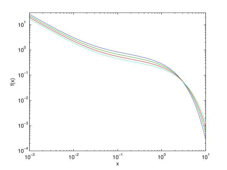
Figure 1: Plots of the PDF $f(x)$ (36) for $n=0.9$, $\theta=0.03$, for different threshold magnitudes $m-m_{1}=0;2;4;6$ (top to bottom on the left), where the reference parameter is $\epsilon_{1}=\lambda_{1}c=10^{-4}$ for $m_{1}$.

Consider for instance $m_{2}-m_{1}=4$, for which the average rate changes by the huge factor $10^{-4}$ while the $\rho\simeq 0.76$ still remains rather close to $1$ for $\theta=0.03$. Fig. 1 plots the PDF $f(x)$ given by (36) for $n=0.9$, $\theta=0.03$ and for different magnitude thresholds $m$. This figure demonstrates the slow dependence of $f(x)$ with respect to magnitude threshold level $m$.

While the plots of the approximate scaling law (36) shown in Fig. 1 differ significantly from Molchan’s exponential unified law, they are close to the parameterization of the empirical PDF proposed by Corral (2004a)

$$f_{c}(x)={C\delta\over d~{}\Gamma(\gamma/\delta)}\left({x\over a}\right)^{\gamma-1}e^{-(x/a)^{\delta}}~{},$$ (38)

with the parameters

$$\gamma=0.67\pm 0.05~{},\qquad\delta=1.05\pm 0.05~{},\qquad a=1.64\pm 0.15~{},$$ (39)

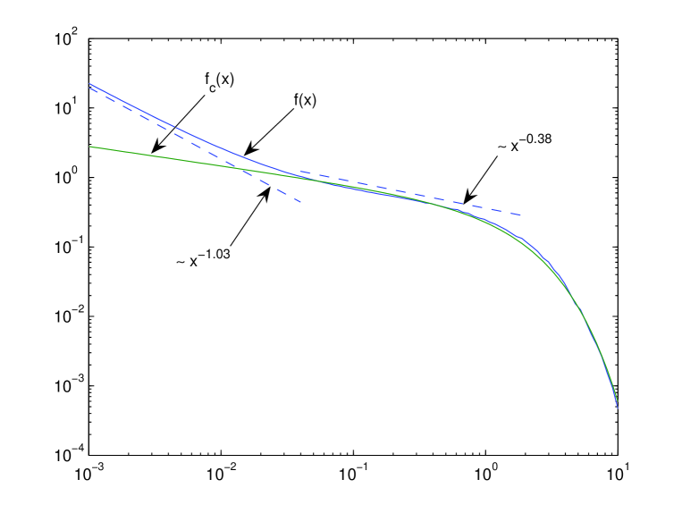
Figure 2: Plot of the PDF $f(x)$ given by expression (36) for the parameters $n=0.9$, $\theta=0.03$, $\epsilon_{1}=0.76$, $m-m_{1}=2$, and Corral’s fitting curve (38) for $\gamma=0.38$, $\delta=1$, $d=1.7$ and $C=0.75$. We also show an intermediate asymptotics $\sim 1/x^{0.38}$ discussed by Corral (see below) as well as the short-time asymptotics $\sim 1/x^{1.03}$ corresponding to the Omori law.

and with a normalization factor $C$ close to 1. Fig. 2 shows a typical PDF $f(x)$ obtained from our expression (36) together with Corral’s fitting curve (38), illustrating their closeness for not too small $x$’s. The two expressions depart for very small $x\lesssim 0.01$, for which our simplified model distribution $f(x)$ given by (36) exhibits a power asymptotic $f(x)\sim x^{-1-\theta}$, which is a direct consequence of the Omori law. This asymptotic term results explicitely from the first term in the factor multiplying $\varphi(x,\epsilon)$ in expression (36). This asymptotic is absent in Corral’s fitting function $f_{c}(x)$ given by (38), although it actually exists in real data plots (Corral, 2004a). We will emphasize this point later when we discuss the full theory and its comparison with the empirical data.

4 Description of the statistics of observable events in the context of the ETAS model

In the preceding sections, we have made plausible and intuitively appealing the possibility that an approximate unified law indeed exists for the PDF of the inter-earthquake times, by using a simplified transparent model of the statistics of recurrence times. In this section, we develop an accurate mathematical description of the statistical properties of observable events, in the framework of the ETAS model presented in the introduction. The technology developed here will then be used in the next section to quantify precisely the prediction of the ETAS model of the PDF of inter-event times and to derive different approximations.

Our analysis is based on our previous calculations (Saichev and Sornette, 2006a), which showed that, for large domain sizes ($L\sim$ tens of kilometers or more), one may neglect the impact of aftershocks triggered by events that occurred outside the considered spatial domain $S$, while only considering the events within the space domain which are triggered by sources also within the same domain. In this approximation validated by precise calculations in (Saichev and Sornette, 2006a), the analysis of the statistical properties of time sequence of earthquakes can be reduced to the study of a time-only version of the ETAS model, in which the dependence on the spatial extension of a given area can be taken into account via the dependence on $L$ of the rate $\omega$ of spontaneous observable events.

As the ETAS model has an exact representation in terms of branching clusters (Hawkes and Oakes, 1974; Helmstetter and Sornette, 2002), the main mathematical tool to analyze the ETAS model in this context is the Generating Probability Function (GPF) of the random number $R(t,\tau,m)$ of observable events within the time interval $[t,t+\tau]$

$$\Omega(z;\tau,m)=\langle z^{R(t,\tau,m)}\rangle~{}.$$ (40)

Here and below, the angle brackets $\langle\dots\rangle$ represent the procedure of statistical averaging. We assume that the process of earthquake triggering is stationary, so that the GPF given by (40) does not depend on $t$ but only on the duration $\tau$ of the time interval $[t,t+\tau]$. Let $P(r,\tau,m)$ be the probability that the number $R(t,\tau,m)$ of observable events is equal to $r$. Then, one may rewrite the definition (40) in the equivalent form

$$\Omega(z;\tau,m)=\sum_{r=0}^{\infty}P(r;\tau,m)z^{r}~{}.$$ (41)

It follows that the probability that no event occurs in a time interval of duration $\tau$ is equal to

$$P(\tau)=P(r=0,\tau,m)=\Omega(0;\tau,m)~{}.$$ (42)

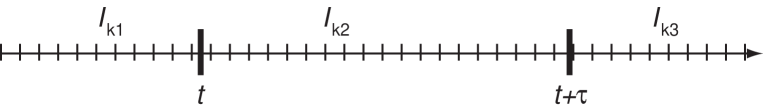
Figure 3: Partition of the time axis in small intervals which are classified in three categories $I_{k_{1}},I_{k_{2}}$ and $I_{k_{3}}$.

To determine the GPF $\Omega(z;\tau,m_{0})$ associated with the total number of events inside the time window $[t,t+\tau]$, we proceed as follows. We partition the $t$-axis in small intervals $I_{k}=[t_{k},t_{k}+\Delta]$ as shown in Fig. 3 and then group them in three categories: the first one $I_{k_{1}}\in(-\infty,t)$ lies before the time window $[t,t+\tau]$ of interest, the second one $I_{k_{2}}\in[t,t+\tau]$ groups all small intervals inside the time window $[t,t+\tau]$ and the third one $I_{k_{3}}\in(t+\tau,\infty)$ lies after the time window $[t,t+\tau]$. Let us now determine in turn the impacts of the spontaneous events occurring within each of these three intervals on the GPF of the number of events inside the time window $[t,t+\tau]$. Let $\Theta_{k_{1}}(z;,m_{0})$ be the GPF of the number of spontaneous events occurring in the first class $I_{k_{1}}$ of small intervals. It is equal to

$$\Theta_{k_{1}}(z;m_{0})=\sum_{r=0}^{\infty}\mathcal{P}(r,\Delta)z^{r}~{},$$ (43)

where $\mathcal{P}(r,\Delta)$ is the Poissonian probability that $r$ spontaneous events occur in $I_{k_{1}}$. It is given by

$$\mathcal{P}(r,\Delta)={(\omega\Delta)^{r}\over r!}e^{-\omega\Delta}~{}.$$ (44)

Let us recall that, according to the ETAS model, spontaneous and triggered events have statistically independent magnitudes whose PDF is to GR law

$$p(m)=-{dQ(m)\over dm}=10^{-b(m-m_{0})}b\ln 10~{}.$$ (45)

Thus, the spontaneous earthquakes have statistically independent magnitudes $\{m_{j}\}$, $j=1,2,\dots,r$. According to the branching property of the ETAS model (Hawkes and Oakes, 1974; Helmstetter and Sornette, 2002), these spontaneous events trigger statistically independent numbers $R_{j}(t_{k},t,\tau,m_{j},m_{0})$ of events within time interval $[t,t+\tau]$. This remark allows us to obtain the GPF $\Omega_{k_{1}}(z;\tau,m_{0})$ of the random number of events within $[t,t+\tau]$ triggered by spontaneous events which occurred inside a given small interval $I_{k_{1}}$: by replacing in (43) the term $z^{r}$ by

$$\left[\int_{m_{0}}^{\infty}p(m^{\prime})\Theta(z;t_{k_{1}}-t,\tau,m^{\prime},m_{0})dm^{\prime}\right]^{r}~{},$$ (46)

using the expression (44) and performing the summation yields

$$\Omega_{k_{1}}(z;\tau,m_{0})=\exp\left(\omega\Delta\left[\int_{m_{0}}^{\infty}p(m^{\prime})\Theta(z;t_{k_{1}}-t,\tau,m^{\prime},m_{0})dm^{\prime}-1\right]\right)~{}.$$ (47)

Here,

$$\Theta(z;t_{k_{1}},\tau,m^{\prime},m_{0})=\langle z^{R(t_{k_{1}},t,\tau,m^{\prime},m_{0})}\rangle$$ (48)

is the GPF of the random numbers of events triggered inside the time interval $[t,t+\tau]$ by some spontaneous event of magnitude $m^{\prime}$ which occurred at a time $t_{k_{1}}<t$. Due to the statistical independence of the random numbers of events triggered by different spontaneous events which belong to different small intervals $I_{k_{1}}$, the GPF of the random numbers of events (including all their “aftershocks”), triggered within the interval $[t,t+\tau]$ by spontaneous events which occurred before the window $[t,t+\tau]$, is equal to

$$\begin{array}[]{c}\displaystyle\Omega_{1}(z;\tau,m_{0})=\prod_{k_{1}}\Omega_{k_{1}}(z;t_{k_{1}}\tau,m_{0})=\\[8.53581pt] \displaystyle\exp\left(\omega\Delta\sum_{k_{1}}\left[\int_{m_{0}}^{\infty}p(m^{\prime})\Theta(z;t_{k_{1}}-t,\tau,m^{\prime},m_{0})dm^{\prime}-1\right]\right)~{}.\end{array}$$ (49)

In the limit $\Delta\to 0$, the discrete sum in the exponential becomes an integral, which yields

$$\Omega_{1}(z;\tau,m_{0})=\exp\left(\omega\int_{-\infty}^{t}dt^{\prime}\left[\int_{m_{0}}^{\infty}p(m^{\prime})\Theta(z;t^{\prime}-t,\tau,m^{\prime},m_{0})dm^{\prime}-1\right]\right)~{}.$$ (50)

Analogously, one can find the GPF $\Omega_{2}(z;\tau,m_{0})$ of the number of windowed events (including all their “aftershocks”) triggered by spontaneous events which occurred within the interval $[t,t+\tau]$. It reads

$$\Omega_{2}(z;\tau,m_{0})=\exp\left(\omega\int_{t}^{t+\tau}dt^{\prime}\left[\int_{m_{0}}^{\infty}p(m^{\prime})z\Theta(z;t+\tau-t^{\prime},m^{\prime},m_{0})dm^{\prime}-1\right]\right)~{},$$ (51)

where

$$\Theta(z;\tau,m^{\prime},m_{0})=\Theta(z;t=0,\tau,m^{\prime},m_{0})$$ (52)

is the GPF of the random number of events triggered inside the interval $t\in[0,\tau]$ by a spontaneous event which occurred at $t=0$.

For the third contribution from spontaneous sources in $I_{k_{3}}\in(t+\tau,\infty)$, the causality principle implies that $\Theta_{k_{3}}\equiv 1$.

Thus, the whole GPF of the numbers of events occurring within the time interval $[t,t+\tau]$ is $\Omega(z;\tau,m_{0})=\Omega_{1}(z;\tau,m_{0})\Omega_{2}(z;\tau,m_{0})$, which can be written

$$\Omega(z;\tau,m_{0})=e^{-\omega L(z;\tau,m_{0})}~{},$$ (53)

where

$$\begin{array}[]{c}\displaystyle L(z;\tau,m_{0})=\int_{m_{0}}^{\infty}dm^{\prime}p(m^{\prime})\times\\[8.53581pt] \displaystyle\left(\int_{0}^{\infty}\left[1-\Theta(z;t,\tau,m^{\prime},m_{0})\right]dt+\int_{0}^{\tau}\left[1-z\Theta(z;t,m^{\prime},m_{0})\right]dt\right)~{}.\end{array}$$ (54)

In order to calculate GPF $\Omega(z;,\tau,m_{0})$ given by (53), (54), we need to determine the GPF $\Theta(z;t,\tau,m^{\prime},m_{0})$ of the number of events triggered within $[t,t+\tau]$ by some spontaneous event magnitude $m^{\prime}$ which occurred at $t^{\prime}=0$. Using a similar procedure as just done for $\Omega(z;\tau,m_{0})$ and interpreting the Omori law (3) as the PDF of random times of independently triggered aftershocks, we obtain

$$\begin{array}[]{c}\Theta(z;t,\tau,m^{\prime},m_{0})=\displaystyle\exp\Big{(}-\rho(m^{\prime})\int_{m_{0}}^{\infty}dm^{\prime\prime}p(m^{\prime\prime})\times\\[8.53581pt] \displaystyle\left[b(t+\tau)-z\Phi(t+\tau)\otimes\Theta(z;\tau,m^{\prime\prime},m_{0})-\Phi(t)\otimes\Theta(z;t,\tau,m^{\prime\prime},m_{0})\right]\Big{)}~{}.\end{array}$$ (55)

The symbol $\otimes$ denotes the convolution operator. We also define

$$b(t)=1-a(t)~{},$$ (56)

where $a(t)$ is given by (28). Similarly, $\Theta(z;\tau,m^{\prime},m_{0})$ satisfies to the equation

$$\begin{array}[]{c}\Theta(z;\tau,m^{\prime},m_{0})=\\[8.53581pt] \exp\left(-\rho(m^{\prime})\displaystyle\int_{m_{0}}^{\infty}dm^{\prime\prime}p(m^{\prime\prime})\left[b(\tau)-z\Phi(\tau)\otimes\Theta(z;\tau,m^{\prime\prime},m_{0})\right]\right)~{}.\end{array}$$ (57)

The above GPF’s take into account events which have arbitrary magnitudes $m^{\prime}\geqslant m_{0}$. In order to get the GPF (40) which only counts observable events with magnitudes larger than some threshold level $m$, one has to replace (i) $m_{0}$ by $m$ in the r.h.s of expressions (53) and (54) and (ii) $z$ by

$$z(m^{\prime},m)=H(m-m^{\prime})+zH(m^{\prime}-m)~{},$$ (58)

where $H(x)$ is unit step (Heaviside) function. We also replace the GPF $\Theta(z;t,\tau,m^{\prime},m_{0})$ by the GPF $\Theta(z;t,\tau,m^{\prime},m)$ of the number of observable aftershocks (whose magnitudes are larger than $m$), triggered by a mainshock of magnitude $m^{\prime}$. We thus obtain

$$\Omega(z;\tau,m)=e^{-\omega L(z;\tau,m)}~{},$$ (59)

where

$$\begin{array}[]{c}\displaystyle L(z;\tau,m)=\int_{0}^{\infty}[1-D(z;t,\tau,m)]dt+\\[8.53581pt] \displaystyle\int_{0}^{\tau}[1-D(z;t,m)+(1-z)D_{+}(z;t,m)]dt\end{array}$$ (60)

and

$$\begin{array}[]{c}\displaystyle D(z;t,\tau,m)=\int_{m_{0}}^{\infty}\Theta(z;t,\tau,m^{\prime},m)p(m^{\prime})dm^{\prime}~{},\\[8.53581pt] \displaystyle\displaystyle D(z;\tau,m)=\int_{m_{0}}^{\infty}\Theta(z;\tau,m^{\prime},m)p(m^{\prime})dm^{\prime}~{},\\[8.53581pt] \displaystyle\displaystyle D_{+}(z;\tau,m)=\int_{m}^{\infty}\Theta(z;\tau,m^{\prime},m)p(m^{\prime})dm^{\prime}~{}.\end{array}$$ (61)

It follows from (55) and (57), after replacing the GPF $\Theta(z;,t,\tau,m^{\prime},m_{0})$ by $\Theta(z;,t,\tau,m^{\prime},m)$, the GPF $\Theta(z;\tau,m^{\prime},m_{0})$ by $\Theta(z;\tau,m^{\prime},m)$ and $z$ by $z(m^{\prime\prime},m)$ (58), that the above auxiliary functions satisfy the equations

$$\begin{array}[]{c}\displaystyle D(z;t,\tau,m)=\Psi\big{[}b(t+\tau)-\Phi(t)\otimes D(z;t,\tau,m)\\[8.53581pt] \displaystyle-\Phi(t+\tau)\otimes D(z;\tau,m)+(1-z)\Phi(t+\tau)\otimes D_{+}(z;\tau,m)\big{]}\end{array}$$ (62)

and

$$\begin{array}[]{c}D(z;\tau,m)=\Psi\big{[}b(\tau)-\Phi(\tau)\otimes D(z;\tau,m)+(1-z)\Phi(\tau)\otimes D_{+}(z;\tau,m)\big{]}~{},\\[8.53581pt] D_{+}(z;\tau,m)=\Psi_{+}\big{[}b(\tau)-\Phi(\tau)\otimes D(z;\tau,m)+(1-z)\Phi(\tau)\otimes D_{+}(z;\tau,m)\big{]}~{}.\end{array}$$ (63)

Here,

$$\begin{array}[]{c}\displaystyle\Psi(y)=\int_{m_{0}}^{\infty}p(m^{\prime})e^{-\rho(m^{\prime})y}dm^{\prime}=\gamma(\kappa y)^{\gamma}\Gamma(-\gamma,\kappa y)~{},\\[11.38109pt] \displaystyle\Psi_{+}(y)=\int_{m}^{\infty}p(m^{\prime})e^{-\rho(m^{\prime})y}dm^{\prime}=Q(m)\Psi[Q^{-1/\gamma}(m)y]~{}.\end{array}$$ (64)

For our following calculations, it is useful to expand $\Psi(y)$ into a power series with respect to $y$:

$$\Psi(y)\simeq 1-ny+\beta y^{\gamma}-\eta y^{2}~{},$$ (65)

where

$$n={\kappa\gamma\over\gamma-1}~{},\quad\beta=-\left(n{\gamma-1\over\gamma}\right)^{\gamma}\Gamma(1-\gamma)~{},\quad\eta={n^{2}(\gamma-1)^{2}\over 2\gamma(2-\gamma)}~{}.$$ (66)

Recall that $n$ is the so-called branching parameter (which we used to obtain expression (24)), defined as the average of the total number of first-generation aftershocks triggered by some mainshock.

Equations (62) and (63) are rather complicated nonlinear integral equations. For the rest of this section, we use them together with expressions (59), (60) only to derive the average number of observable earthquakes. In the next sections, we exploit them fully to obtain the PDF of the inter-event times.

As recalled for instance in the Appendix of (Saichev and Sornette, 2006a), the usefulness of the theory of GPF is to obtain simple expressions for the average number of observable earthquakes:

$$\langle R(t,\tau,m)\rangle={d\Omega(z;\tau,m)\over dz}\Big{|}_{z=1}~{}.$$ (67)

Using (59), (60), this leads to

$$\langle R(t,\tau,m)\rangle=\omega Q(m)\tau+\omega\int_{0}^{\infty}M(t,\tau,m)dt+\omega\int_{0}^{\tau}M(\tau,m)dt~{},$$ (68)

where

$$M(t,\tau,m)={dD(z;t,\tau,m)\over dz}\Big{|}_{z=1}~{},\quad M(\tau,m)={dD(z;\tau,m)\over dz}\Big{|}_{z=1}~{}.$$ (69)

The functions in (69) satisfy the following equations derived from (62) and (63):

$$\begin{array}[]{c}M(t,\tau,m)-n\Phi(t)\otimes M(t,\tau,m)=\\[8.53581pt] =n\Phi(t+\tau)\otimes M(\tau,m)+n\left[a(t)-a(t+\tau)\right]Q(m)\end{array}$$ (70)

and

$$M(\tau,m)-n\Phi(\tau)\otimes M(\tau,m)=nb(\tau)Q(m)~{}.$$ (71)

It follows from (70) that the following equality is true

$$(1-n)\int_{0}^{\infty}M(t,\tau,m)dt=na(\tau)\otimes M(\tau,m)+nQ(m)A(\tau)~{}.$$ (72)

Using this equality in (68), we obtain

$$\begin{array}[]{c}\langle R(t,\tau,m)\rangle=\\[8.53581pt] \displaystyle\omega\left[Q(m)\tau+{n\over 1-n}Q(m)A(\tau)+{n\over 1-n}a(\tau)\otimes M(\tau,m)+\int_{0}^{\tau}M(t,m)dt\right]~{},\end{array}$$ (73)

where $A(\tau)$ is given by (30).

Using equation (71), it is easy to show that

$${n\over 1-n}a(\tau)\otimes M(\tau,m)+\int_{0}^{\tau}M(\tau,m)dt={n\over 1-n}Q(m)\tau-{n\over 1-n}Q(m)A(\tau)~{}.$$ (74)

This leads to

$$\langle R(t,\tau,m)\rangle={\omega(m)\over 1-n}\tau~{},\qquad\omega(m)=\omega Q(m)~{},$$ (75)

which has a physically intuitive interpretation: the average number of observable events is equal to average number of observable spontaneous events $\omega(m)\tau$ within the interval of duration $\tau$, multiplied by the factor $1/(1-n)$ taking into account all the triggered “aftershocks” of all generations. The result (75) which can be obtained more directly (Helmstetter and Sornette, 2002; 2003c) serves as a consistency check of our GPF formalism.

5 Statistics of recurrence times in the context of the ETAS model: accounting for Corral’s empirical analyses

We now use the formalism developed in the preceding section to derive the probability $P(\tau)$ given by (42) that no event occurs with a time interval of duration $\tau$. Using (59), (60), (61), it is equal to

$$P(\tau)=e^{-\omega L(\tau,m)}~{},$$ (76)

where

$$L(\tau,m)=\int_{0}^{\infty}N(t,\tau,m)dt+\int_{0}^{\tau}N_{-}(t,m)dt$$ (77)

and

$$\begin{array}[]{c}\displaystyle N(t,\tau,m)=1-D(t,\tau,m)~{},\\[8.53581pt] \displaystyle N_{-}(\tau,m)=1-D(\tau,m)+D_{+}(\tau,m)~{}.\end{array}$$ (78)

These functions have a clear probabilistic interpretation. For instance, $N(t,\tau,m)$ is the probability that some spontaneous earthquake, which occurred at time $t=0$, will trigger at least one observable event (which can be an aftershock of arbitrary generation) within the time window $[t,t+\tau]$ ($t>0$).

It follows from (62) that the probability $N(t,\tau,m)$ satisfies the equation

$$\begin{array}[]{c}N(t,\tau,m)=\\[8.53581pt] 1-\Psi\left[\Phi(t)\otimes N(t,\tau,m)+\Phi(t+\tau)\otimes N_{-}(\tau,m)\right]~{}.\end{array}$$ (79)

Analogously, it follows from (63) that $N_{-}(\tau,m)$ satisfies the equation

$$\begin{array}[]{c}N_{-}(\tau,m)=\\[8.53581pt] \displaystyle 1-\Psi\left[\Phi(\tau)\otimes N_{-}(\tau,m)\right]+Q(m)\Psi\left[Q^{-1/\gamma}(m)\Phi(\tau)\otimes N_{-}(\tau,m)\right]~{}.\end{array}$$ (80)

These are still rather complicated nonlinear integral equations. We can simplify them by linearization, which provides a reasonable approximation, as can be seen from the following argument. First, we notice that the inequalities obviously hold

$$N(t,\tau,m)<N(m)~{},\qquad N_{-}(\tau,m)<N_{-}(m)~{},$$ (81)

where

$$N(m)=N(t=0,\tau=\infty,m)~{},\qquad N_{-}(m)=N_{-}(\tau=\infty,m)~{}.$$ (82)

The majorants $N(m)$ and $N_{-}(m)$ satisfy the following nonlinear functional equations derived from from (79), (80):

$$\begin{array}[]{c}N(m)=1-\Psi[N_{-}(m)]~{},\\[8.53581pt] N_{-}(m)=1-\Psi[N_{-}(m)]+Q(m)\Psi[Q^{-1/\gamma}(m)N_{-}(m)]~{}.\end{array}$$ (83)

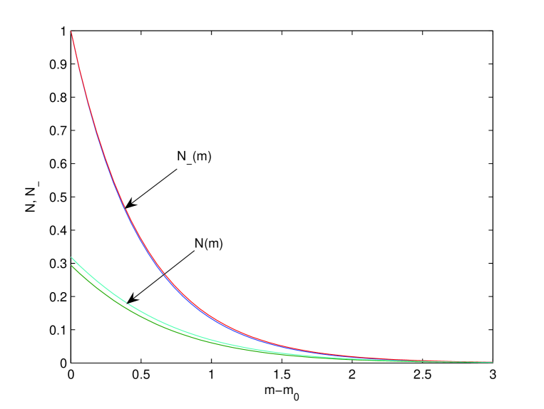
Figure 4: Plots of the solutions of the nonlinear functional equations (83) for $N(m)$ and $N_{-}(m)$, for the parameters $\gamma=1.2$ and two values of criticality parameter $n=0.8;0.9$.

We have solved numerically these equations (83) and Fig. 4 plots these solutions for $N(m)$ and $N_{-}(m)$. One can observe that, even for moderate magnitude thresholdss $m-m_{0}\gtrsim 1$, both $N(m)\ll 1$ and $N_{-}(m)\ll 1$, so that, with the inequalities (81), one can be confident that a linear approximation of the r.h.s. of equations (79), (80) should provide a good approximation.

The linear approximation of equations (79) and (80) amounts to replace the function $\Psi(y)$ defined in (64) by the first two terms of the expansion (65):

$$\Psi(y)\approx 1-ny~{}.$$ (84)

This approximation (84) has a transparent probabilistic interpretation. It corresponds to assuming that any given earthquake can either trigger no or just one observable aftershock of first-generation. However, through the avalanche process of aftershocks which themselves trigger no or just one aftershock, the total average number $\langle R\rangle=n/(1-n)$ of aftershocks over all generations which are triggered by a given mainshock can still be large for $n$ close to $1$. A possible justification of the approximation that no more than one observable first-generation aftershock is triggered by a given event is that this statement refers to observable aftershocks with magnitudes above the threshold level $m>m_{0}$. For $m$ large enough above $m_{0}$, a given mainshock may trigger many aftershocks of first generation of magnitude larger than $m_{0}$, but few of them will be observable with magnitudes larger than $m$, due to the fast decay of the GR PDF (2) with increasing $m$. This effect has been shown to lead to a renormalization of the branching ratio $n$ into an apparent value $n_{a}\leq n$ (the equality holding only for the two fixed points $n=0$ and $n=1$), characterizing the apparent branching structure of the triggering of observable events (Sornette and Werner, 2005b; Saichev and Sornette, 2006b).

With the linear approximation (84), equation (80) takes the form

$$N_{-}(\tau,m)=Q(m)+\delta\Phi(\tau)\otimes N_{-}(\tau,m)~{},$$ (85)

where

$$\delta=n[1-Q^{\gamma-1\over\gamma}(m)]~{}.$$ (86)

Similarly, expression (79) allows us to obtain

$$N(t,\tau,m)=n\Phi(t)\otimes N(t,\tau,m)+n\Phi(\tau+t)\otimes N_{-}(\tau,m)~{}.$$ (87)

Integrating the expression (84) term by term over time yields

$$\int_{0}^{\infty}N(t,\tau,m)dt=n\int_{0}^{\infty}N(t,\tau,m)dt+na(\tau)\otimes N_{-}(\tau,m)~{},$$ (88)

which simplifies into

$$\int_{0}^{\infty}N(t,\tau,m)dt={n\over 1-n}a(\tau)\otimes N_{-}(\tau,m)~{}.$$ (89)

Using (89), we rewrite the probability (76) in the form

$$P(\tau)=\exp\left(-{\omega n\over 1-n}a(\tau)\otimes N_{-}(\tau,m)-\omega\int_{0}^{\tau}N_{-}(t,m)dt\right)~{},$$ (90)

which now involves only the function $N_{-}(t,m)$.

Thus, in order to find the explicit expression for $P(\tau)$ from (90), we need to solve equation (85). We can already state that its solution should obey the following limiting condition

$$\lim_{\tau\to\infty}N_{-}(\tau,m)=N_{-}(m)={Q(m)\over 1-\delta}~{}.$$ (91)

We now introduce the new function

$$g(\tau,m)={N_{-}(\tau,m)\over N_{-}(m)}-1\quad\iff\quad N_{-}(\tau,m)=N_{-}(m)[1-g(\tau,m)]~{}.$$ (92)

It is easy to show that $g(\tau,m)$ satisfies the equation

$$g(\tau,m)-\delta\Phi(\tau)\otimes g(\tau,m)=\delta a(\tau)~{},$$ (93)

from which we derive the following relation

$$a(\tau)\otimes g(\tau,m)=A(\tau)+{\delta-1\over\delta}\int_{0}^{\tau}g(t,m)dt~{}.$$ (94)

Substituting in (90) the second relation of (92) and using (94) yields

$$P(\tau)=\exp\left(-{\omega(m)\tau\over 1-\delta}-{\omega(m)\over\delta}\Delta\int_{0}^{\tau}g(t,m)dt\right)~{},$$ (95)

where

$$\Delta={n\over 1-n}-{\delta\over 1-\delta}$$ (96)

and $\omega(m)=\omega Q(m)$ is the average rate of observable spontaneous events. Recall that $\delta$ is given by (86).

A standard technique to obtain the solution of equation (93) is to use the inverse Laplace transform. It gives

$$g(\tau,m)=g_{0}\left({\tau\over c},m\right)~{},$$ (97)

where

$$g_{0}(z,m)=-{\delta\over\pi}\int_{0}^{\infty}\text{Im}\left({1-\hat{\Phi}(y,\theta)\over y[1-\delta\hat{\Phi}(y,\theta)]}\right)e^{-yz}dy$$ (98)

and

$$\hat{\Phi}(y,\theta)=y^{\theta}e^{y}\Gamma(-\theta,y)~{}.$$ (99)

Due to the extremely slow decay of the function $a(\tau)$ (28) for $\theta\ll 1$, the exact solution (97) of equation (93) can be described accurately by the quasi-static approximation

$$g(\tau,m)\approx{a(\tau)\delta\over 1-\delta+\delta a(\tau)}~{}.$$ (100)

Substituting this quasistatic approximation (100) in expression (95) yields

$$P(\tau)=\exp\left(-{\omega(m)\tau\over 1-\delta}-\omega(m)\Delta\int_{0}^{\tau}{a(t)dt\over 1-\delta+\delta a(t)}\right)~{}.$$ (101)

It is interesting to notice that, for $\delta\ll 1$, one may neglect $\delta$ and replace the expression (101) by

$$P(\tau)\approx\exp\left(-\omega(m)\tau-n{\omega(m)\over 1-n}A(\tau)\right)~{},$$ (102)

which coincides with the simplified model probability (32) derived in section 3. The conditions under which this approximation holds can be visualized from Fig. 5 showing the dependence of of $\delta$, taking as a function of $m-m_{0}$ for different values of $\gamma=b/\alpha$. This dependence results from the competition between the decay of the GR law controlled by its exponent $b$ and the value of the productivity exponent $\alpha$.

Fig. 5 shows that the condition $\delta\ll 1$ needed to obtain (102) requires that $m-m_{0}$ should not be too large, while Fig. 4 has shown that the linear approximation (84) used to obtain these results is all the more valid the larger is $m-m_{0}$. It is thus worthwhile to come back to the more complete expression (101) for $P(\tau)$, which holds for arbitrary values of $\delta$. It is convenient to rewrite (75) so that the average number of windowed events is equal to

$$x=\lambda(m)\tau~{},\qquad\lambda(m)={\omega(m)\over 1-n}~{}.$$ (103)

With these notations, we have

$$P(\tau)=\varphi(x,m)=\exp\left(-\eta x-\nu\int_{0}^{x}g(y,m,\theta)dy\right)~{},$$ (104)

where

$$g(x,m,\theta)={\epsilon^{\theta}\over\delta\epsilon^{\theta}+(1-\delta)(\epsilon+y)^{\theta}}~{}.$$ (105)

and

$$\eta={1-n\over 1-\delta}~{},\quad\nu=(1-n)\Delta~{},\quad\epsilon=c\lambda(m)={c\omega(m)\over 1-n}~{}.$$ (106)

Correspondingly, the sought dimensionless PDF of the recurrence times defined by

$$f(x,m)={d^{2}\varphi(x,m)\over dx^{2}}$$ (107)

is given by

$$\begin{array}[]{c}f(x,m)=\\[8.53581pt] \displaystyle\left(\theta\nu(1-\delta)\epsilon^{-\theta}(x+\epsilon)^{\theta-1}g^{2}(x,m,\theta)+\left[\eta+\nu g(x,m,\theta)\right]^{2}\right)\varphi(x,m)~{}.\end{array}$$ (108)

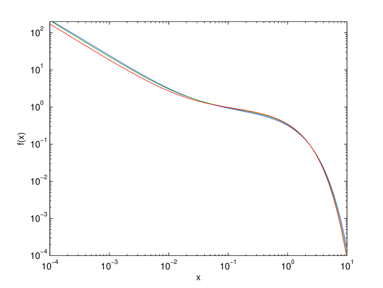
Figure 6: Plots of the PDF (108) of the scaled recurrence times $x$ for $\theta=0.03$, $\gamma=1.2$, $n=0.9$ and for different magnitude thresholds $m-m_{0}=2,4,6$.

Similarly to the observation that the simplified version (36) for the PDF of recurrence times depends very slowly on the magnitude threshold $m$, the PDF of inter-event times (108) predicted by the ETAS model also depends weakly on $m$, if $\theta\ll 1$ and $\gamma$ is close to $1$. Fig. 6 plots the dependence of the PDF (108) as a function of the dimensionless inter-event time $x$ for $\theta=0.03$, $\gamma=1.2$ and $n=0.9$ for different magnitude thresholds $m=2,4,6$. For such a span of magnitude thresholds, the average rate (103) changes by many orders of magnitudes, while the corresponding PDF’s are amazingly close each other. Fig. 6 indeed examplifies the very weak dependence of the PDF on $m$.

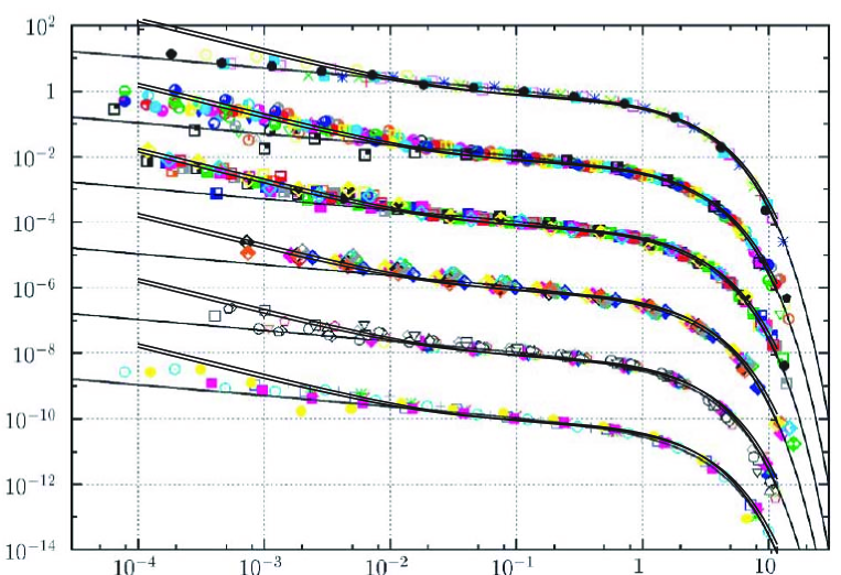
Figure 7: Plots of the empirical PDF’s of scaled inter-event times taken from (Corral, 2004a), Corral’s fitting curves using expression (38) (single solid curves) and our theoretical prediction (108) for $\theta=0.03$, $\gamma=1.2$ and $n=0.9$ (double solid curves). Our ETAS prediction is shown as double solid curves because we show the theoretical prediction (108) for two different magnitude threshold levels $m-m_{0}=2$ and $6$, showing the very weak dependence on the magnitude of completeness. Top to bottom: the NEIC worldwide catalog for regions with $L\geq 180$ degrees, 1973-2002; NEIC with $L\leq 90$ degrees, (same period of time); Southern California, 1984-2001, 1988-1991, and 1995-1998; Northern California, 1998-2002; Japan, 1995-1998, and New Zealand, 1996-2001; (bottom), Spain, 1993-1997, New Madrid, 1975-2002, and Great Britain, 1991-2001. The curves are translated for clarity by the factors $1;10^{-2};10^{-4};10^{-6};10^{-8}$ and $10^{-10}$ from top to bottom.

Fig. 7 shows the empirical PDF’s of the scaled inter-event times constructed by Corral (2004a), as well as Corral’s fitting curves using expression (38). We superimpose on these curves our theoretical prediction (108), which actually provides a better fit to the data, especially for small $x\lesssim 10^{-2}$, where our ETAS prediction correctly accounts for the impact of Omori’s law, as already mentioned in our discussion of the simplified model PDF (36). We present the theoretical prediction (108) for two different magnitude threshold levels $m-m_{0}=2$ and $6$, showing the very weak dependence on the magnitude of completeness. These results suggest that the parameter $\theta$ of the (bare) Omori law needs to be small (typically $\theta\lesssim 0.1$) to account for the data. Similar fits are obtained for the range of parameters $1<\gamma\leq 1.2$ and $0.8\leq n<1$, in agreement with bounds previously obtained from the prediction of the ETAS model on the distribution of seismic rates (Saichev and Sornette, 2006a).

6 PDF of recurrence times for multiple regions: accounting for Bak et al. (2002)’s empirical analysis

Until now, we have derived the prediction of the ETAS model for the statistics of inter-event times in a single homogeneous region and have shown that it is compatible with the empirical observation of an approximate unified scaling law of the form (5). We have also shown that our theoretical expression fits remarkably well the empirical PDF’s over the whole range of recurrence times, accounting for different regimes by using only the physics of triggering quantified by Omori’s law.

There is another unified saling law for the statistics of recurrence time obtained after averaging over multiple regions, which has been proposed by Kossobokov and Mazhkenov (1988) and Bak et al. (2002). We will refer for short to this law as Bak et al.’s unified law. The aim of this section is to derive analytically Bak et al.’s unified law obtained for multiple regions based on the prediction of the ETAS model that we have presented in the previous section and on the simple hypothesis that all regions obey the PDF form (108) but with different average seismic rates. This simply means that Bak et al.’s unified law in our view just results from an appropriate averaging of expression (108) over the statistics of the average rates of the multiple regions under observation.

We first present in subsection 6.1 a general scheme to perform this averaging in the next subsection with various test statistics for the average rates in different regions. Then, in the second subsection 6.2, we introduce a fractal geometrical model which allows us to propose a specific statistics for the average rates in different regions, which lead to excellent fits to the empirical data.

6.1 General statistics for the average regional seismic rates

In order to choose reasonable statistics for the average seismic rates $\omega_{i}$ in multiple regions with the minimum of additional parametes, we assume that these $\omega_{i}$’s obey a principle of statistical self-similarity: if the branching ratios $n_{i}$’s and the linear size $L_{i}$’s of different regions are identical, then the seismic rates can be written

$$\omega_{i}=\bar{\omega}~{}u_{i}~{},$$ (109)

where $\bar{\omega}$ is the rate of spontaneous events averaged over all regions, while the $u_{i}$’s are mutually independent random variables distributed according to the same PDF $\mathcal{E}(u)$. The PDF $\mathcal{E}(u)$ is assumed to be independent of the common values of the branching ratio $n$ and linear size $L$ of the multiple regions. Additionally, we assume that, as for the scaling law (5) of a single region, the PDF $\mathcal{E}(u)$ does not depend on the magnitude threshold $m$ (which is common to all regions). One may interpret this assumption as a consequence of the scaling properties of the GR law.

Since the average rates of spontaneous events cannot be directly observed, it may be preferable to replace the statement (109) by the equivalent representation

$$\lambda_{i}=\bar{\lambda}~{}u_{i}~{},$$ (110)

which involves the total observable seismic rates above a magnitude threshold. Due to (110), the PDF $\mathcal{E}(u)$ should satisfy to double normalization condition

$$\int_{0}^{\infty}\mathcal{E}(u)du=\int_{0}^{\infty}u\mathcal{E}(u)du\equiv 1~{}.$$ (111)

In this subsection, we concentrate our attention on the universal properties of the PDF of recurrence times constructed over multiple regions, which are found almost the same for qualitatively different distributions $\mathcal{E}(u)$. In the next subsection 6.2, we will obtain a specific expression for the PDF $\mathcal{E}(u)$ from a simple model based on a fractal distribution of spontaneous earthquake sources.

Applying our conjecture (110) to the general relation (10), the PDF of inter-event times over multiple regions is obtained as

$$\mathcal{H}(\tau)={1\over\rule{0.0pt}{11.38109pt}\bar{\lambda}}{d^{2}\over d\tau^{2}}\int_{0}^{\infty}P(\tau)\mathcal{E}(u){du\over u}~{},\qquad\bar{\lambda}={\bar{\omega}\over 1-n}~{}.$$ (112)

It is convenient to represent the probability $P(\tau)$ given by (76) that no events occur in a given single region in the form

$$P(\tau)=e^{-uK(x)}~{},$$ (113)

where the auxiliary function

$$K(x)=\bar{\omega}L\left({x\over\bar{\lambda}},m\right)~{},\qquad x=\bar{\lambda}\tau~{},$$ (114)

does not depend on $u$. It follows from (101) that

$$K(x)=\eta x+\nu\int_{0}^{x}g(y,m,\theta)dy~{},$$ (115)

where $g(y,m,\theta)$ is given by (105). Substituting (113) into (112) yields the following expression analogous to (1) for the PDF of the recurrence times over multiple regions:

$$\mathcal{H}(\tau)=\bar{\lambda}h(\bar{\lambda}\tau)$$ (116)

where

$$h(x)=\left({dK(x)\over dx}\right)^{2}\hat{\mathcal{E}}_{1}(K(x))-{d^{2}K(x)\over dx^{2}}\hat{\mathcal{E}}(K(x))~{}.$$ (117)

We have used the following Laplace transforms

$$\hat{\mathcal{E}}(x)=\int_{0}^{\infty}\mathcal{E}(u)e^{-ux}du~{},\quad\hat{\mathcal{E}}_{1}(x)=-{d\hat{\mathcal{E}}(x)\over dx}=\int_{0}^{\infty}u\mathcal{E}(u)e^{-ux}du~{}.$$ (118)

It is possible to derive the following asymptotic behavior of the PDF $h(x)$ (117). Below, we will illustrate the main features of these asymptotics using the limiting case $\delta=0$ and $\tau\gg c$ such that $K(x)$ reduces to

$$K(x)\approx(1-n)x+{n\over 1-\theta}\epsilon^{\theta}x^{1-\theta}~{},$$ (119)

corresponding to the simplified model of recurrence time statistics.

Let us first consider the behavior of $h(x)$ for $x\ll 1$. First, the asymptotic behavior of the dimensionless PDF $h(x)$ for $x\ll 1$ is universal in the sense that it does not depend on the shape of the PDF $\mathcal{E}(u)$ of the average rates of the multiple regions. Indeed, due to the double normalization condition (111), we have

$$\mathcal{E}(K)\simeq\mathcal{E}_{1}(K)\simeq 1\qquad(K\ll 1)~{}.$$ (120)

Thus, in view of (117) and (119), we obtain

$$h(x)\approx(1-n+n\bar{\epsilon}^{\;\theta}x^{-\theta})^{2}+\theta n\bar{\epsilon}^{\;\theta}x^{-1-\theta}\qquad(x\ll 1)~{}.$$ (121)

For very small $x$’s, the last term prevails and we have the universal asymptotic

$$h(x)\approx\theta n\bar{\epsilon}^{\;\theta}x^{-1-\theta}~{},\qquad x\ll x_{*}\ll 1~{}.$$ (122)

The range of validity of this asymptotic can be roughly estimated by putting formally $\bar{\epsilon}^{\;\theta}x^{-\theta}\approx 1$ in the r.h.s. of relation (121), which gives

$$h(x)\approx 1+\theta nx^{-1}$$ (123)

so that

$$x_{*}\approx\theta n~{}.$$ (124)

Let us now consider the behavior of $h(x)$ for $x\gg 1$. We observe an almost universal asymptotic of the dimensionless PDF $h(x)$ given by (117) for $x\gg 1$. Indeed, let us assume that the PDF of the average seismic rates of the multiple regions has, for small $u$, the following power asymptotic

$$\mathcal{E}(u)\approx\mu u^{\alpha}~{},\qquad u\ll 1~{}.$$ (125)

This leads to the explicit form of the Laplace transforms (118):

$$\hat{\mathcal{E}}(x)\simeq\mu\Gamma(1+\alpha)x^{-1-\alpha}~{},\qquad\hat{\mathcal{E}}_{1}(x)\simeq\mu\Gamma(2+\alpha)x^{-2-\alpha}~{},\qquad x\gg 1~{}.$$ (126)

This finally yields

$$\begin{array}[]{c}h(x)\approx\mu\Gamma(1+\alpha)\times\\[8.53581pt] \left[(1+\alpha)(1-n+n\bar{\epsilon}^{\;\theta}x^{-\theta})^{2}K^{-2-\alpha}(x)+\theta n\bar{\epsilon}^{\;\theta}x^{-1-\theta}K^{-1-\alpha}(x)\right]~{}.\end{array}$$ (127)

For small $\theta$, the leading behavior of this asymptotic can be obtained by using $K(x)\approx x$, which gives

$$h(x)\sim x^{-2-\alpha}~{}.$$ (128)

A useful overview of the behavior of the dimensionless PDF $h(x)$ valid for all interdiate values $x$, including the two above asymptotics (122) and (128), can be obtained by considering a smoothed function interpolating between them. Let us for instance consider the following modeling function

$$h_{m}(x)={1+\theta nx^{-1-\theta}\over 1+x^{2+\alpha}}~{}.$$ (129)

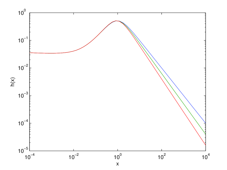
Figure 8: Plots of the function $xh_{m}(x)$ for $\theta=0.03$, $n=0.9$ and for different values of $\alpha=0;0.1,0.2$, demonstrating the approximate unified scaling law of the PDF of inter-event times obtained over multiple regions, as reported by Bak et al. (2002).

We put here for simplicity $\mu\Gamma(2+\alpha)\approx 1$. Fig. 8 shows the function $xh_{m}(x)$ for $\theta=0.03$, $n=0.9$ and for different values $\alpha$, which mimics the empirical construction reported by Bak et al. (2002). Note in particular the existence of a plateau for $x\ll 1$, corresponding to the Omori law asymptotic (122). One can also observe the power law asymptotic $x^{-1-\alpha}$, corresponding to the asymptotic (128) for $x\gg 1$. In addition, there is an intermediate kink for $x\simeq 1$, due to the first term of the asymptotic formula (123). All three features mimic the behavior found by Bak et al. (2002).

These properties of $h(x)$ are weakly dependent on the value of the exponent $\alpha$, which controls the asymptotic behavior (125) of the PDF of the average seismic rates of the multiple regions for small rates. To illustrate this point, consider two qualitatively different sample distributions $\mathcal{E}(u)$ which obey the double normalization (111). Our first example is the Gamma distribution formulated so that it obeys (111):

$$\mathcal{E}^{g}(u)={(1+\alpha)^{1+\alpha}\over\Gamma(1+\alpha)}u^{\alpha}e^{-(1+\alpha)u}~{}.$$ (130)

The main properties of this distribution are the presence of a power asymptotic (125) for small $u$’s and an exponential decay for $u\gg 1$. In this case, the Laplace transforms (118) are

$$\hat{\mathcal{E}}^{g}(x)=\left({1+\alpha\over 1+\alpha+x}\right)^{1+\alpha}~{},\qquad\hat{\mathcal{E}}_{1}^{g}(x)=\left({1+\alpha\over 1+\alpha+x}\right)^{2+\alpha}~{}.$$ (131)

Our second example for a distribution obeying (111) is

$$\mathcal{E}^{p}(u)={p+1\over p}\left(1+{u\over p}\right)^{-2-p}~{},$$ (132)

which corresponds to the particular case $\alpha=0$. The main difference between this distribution and the previous Gamma distribution is the slowly decaying power law tail for $u\gg 1$:

$$\mathcal{E}^{p}(u)\sim u^{-p-2}\qquad(u\gg 1)~{}.$$ (133)

In this case, the Laplace transforms (118) read

$$\hat{\mathcal{E}}^{p}(x)=(1+p)(px)^{1+p}e^{px}\Gamma(-1-p,px)$$ (134)

and

$$\hat{\mathcal{E}}_{1}^{p}(x)={1\over x}\left(1+p-(1+p+px)\mathcal{E}_{p}(x)\right)~{}.$$ (135)

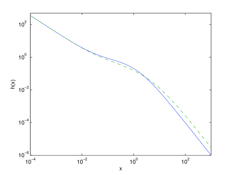
Figure 9: Plots of the PDF $h(x)$ given by(117) for $\theta=0.03$, $n=0.9$, obtained by using the two examples (130) and (132) for the the PDF of the average seismic rates of the multiple regions. Solid line: the Gamma distribution (130) for $\alpha=0$; dashed line: the power tail distribution (132) for $p=0.5$.

Fig. 9 plots the PDF $h(x)$ obtained with the two examples (130) and (132). It would be difficult to distinguish between these two distributions in a realistic empirical setting with limited data and large statistical fluctuations.

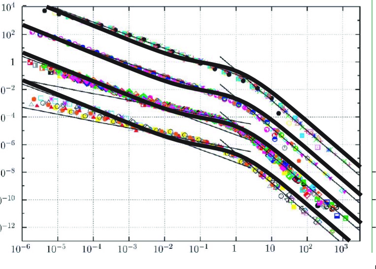
Figure 10: Empirical PDF’s of the recurrence times between earthquakes over multiple regions following Bak et al. (2002)’s procedure obtained from Fig. 2 of (Corral, 2004a), on which has been superimposed our prediction for $h(x)$ obtained with the Gamma distribution (130) for $\mathcal{E}(u)$ with $\theta=0.03$, $n=0.9$, $\epsilon=0.76$ and $\alpha=0.2$. The curves have been translated from top to bottom by the factors $1;10^{-2};10^{-4};10^{-6}$.

In the next subsection 6.2, we develop a simple model for $\mathcal{E}(u)$ based on the idea that seismic rates of spontaneous events are distributed on a fractal geometrical set. In a nutshell, the key idea is the following: a spatial distribution of spontaneous events with fractal dimension $d<2$ implies that, the larger is the number of events, the larger are the spatial distances between them. Thus, the PDF of the number $R$ of events within a given region should decay quite fast at the number of events increases. This tends to favor the decay for large seismic rates modelled by the Gamma distribution (130) over the power law distribution (132). To finish this general discussion, we present in Fig. 10 the empirical data analyses by Corral (2004a) together with prediction for $h(x)$ obtained by using the Gamma distribution for $\mathcal{E}(u)$ with $\theta=0.03$, $n=0.9$, $\epsilon=0.76$ and $\alpha=0.2$. The fits to the empirical data are suggestive as they captures all its qualitative features. There are however undeniable quantitative differences which result in part from the fact that the Gamma distribution is probably not the true distribution for $\mathcal{E}(u)$ even if it captures correctly the mean properties of the data.

6.2 Probabilistic consequences of the fractal geometry of the spatial distribution of spontaneous earthquakes

In the framework of the ETAS model combined with the hypothesis of statistical self-similarity, the preceding subsection 6.1 has stressed that an analytical understanding of Bak et al.’s unified law requires the knowledge of the PDF $\mathcal{E}(u)$ of the average rates over the multiple regions. To constrain its structure, we make the assumption that the well-known fractal spatial organization of all observed earthquakes reflects a similar fractal spatial organization of the subset of spontaneous events which are the origin of the earthquake triggering activity. We thus assume that spontaneous events are distributed spatially on a fractal geometry, which we are going to exploit to derive a natural form for the PDF $\mathcal{E}(u)$.

For this goal, the key idea is based on an important relation between two reciprocal random variables. The first random variable is the area $S(k)$ occupied by $k$ spontaneous events which occurred during a fixed time interval of duration $\tau$. The second random variable $k(S)$ is the inverse function of $S(k)$, which is nothing but the number of spontaneous events within the given area $S$. Although both functions are ill-defined in practice due to the difficulties in defining unambiguously the areas occupied by chaotically occurring disseminated events, we can nevertheless obtain approximate scaling laws for the distributions of these two variables, which derive from the fact that the average $k(S)$, which is proportional to the rate of spontaneous events $\omega(s)$, should obey to power law

$$\langle k(S)\rangle\sim\omega(S)\sim L^{d}~{}.$$ (136)

Here, $L$ is a characteristic scale of the area $S$ and $d$ is the fractal dimension of the spatial set of spontaneous events.

In order to obtain these scaling laws, we recognize that the $i$-th spontaneous event “occupies” a spatial area $s_{i}$ such that, if some area $S$ contains $k$ spontaneous events, then it is equal to

$$S(k)\approx s_{1}+s_{2}+\dots+s_{k}~{}.$$ (137)

One may interpret $s_{i}$ as given by $s_{i}\approx L_{i}^{2}$ where $L_{i}$ is the distance between the $i$-th event and its nearest neighbor. Next, let us assume that the summands in (137) are statistically independent with a common PDF $v(s)$ which has the following aymptotic power law

$$v(s)\approx\eta{d\over\Gamma(1-d)}s^{-1-g}~{},\qquad s\to\infty\qquad 0<g<1~{}.$$ (138)

The expression (138) corresponds to a distribution of spatial jumps, as in a so-called Lévy flights (Metzler and Klafter, 2000), which underlies the fractal spatial distribution of spontaneous events. From the generalized central limit theorem (Gnedenko and Kolmogorov, 1954; Sornette, 2004), the PDF of the random sum (137) for $k\gg 1$ is given asymptotically by

$$V_{k}(s)\approx{1\over(\eta k)^{1/g}}f_{g}\left({s\over(\eta k)^{1/g}}\right)~{},\qquad k\gg 1~{},$$ (139)

where $f_{g}(x)$ is an infinitely divisible distribution, whose Laplace transform is equal to

$$\hat{f}_{g}(y)=\int_{0}^{\infty}f_{g}(x)e^{-yx}dx=e^{-v^{g}}~{},\qquad 0<g<1~{}.$$ (140)

Let us now view expression (137) from a different vantage. One can also interpret (137) as an implicit equation

$$S(k)=S$$ (141)

for the unknown variable equal to the number $k(S)$ of spontaneous events occurring within the given area $S$. Piryatinska et al. (2005) have shown that the PDF of the random variable $S$ allows one to derive the PDF of the random variable $k(S)$ as

$$W(k;S)={\eta\over S^{g}}w_{g}\left({\eta k\over S^{g}}\right)~{},$$ (142)

where

$$w_{g}(x)={1\over gx^{1+1/g}}f_{g}\left({1\over x^{1/g}}\right)~{}.$$ (143)

We then deduce that the average of the random variable $k(S)$ distributed according to the PDF (142) is given by

$$\langle k(S)\rangle={S^{g}\over\eta\Gamma(1+g)}$$ (144)

Since $S\approx L^{2}$ in (144) and comparing with (136) yields the self-consistent determination of the exponent $g$

$$g=d/2~{},$$ (145)

which is indeed between $0$ and $1$ for $0<d<2$. Assuming that average rates of single regions are proportional to $k(S)$, that is $\lambda\sim\omega\sim k(S)$, we obtain

$$\lambda_{i}=\bar{\lambda}u_{i}~{},\qquad u_{i}={k(S_{i})\over\langle k(S)\rangle}~{},$$ (146)

where $S_{i}$ are different regions with the same linear size $L$. The sought PDF of the average seismic rates is thus equal to

$$\mathcal{E}(u)={1\over\bar{u}}w_{d/2}\left({u\over\bar{u}}\right)~{},\qquad\bar{u}=\Gamma(1+d/2)~{}.$$ (147)

One can show that

$$\begin{array}[]{c}w_{g}(u)=\\[8.53581pt] \displaystyle{1\over\pi g}\int_{0}^{\infty}\exp\left[x^{1/g}\cos\left({\pi\over 2g}\right)\right]\cos\left[ux-x^{1/g}\sin\left({\pi\over 2g}\right)\right]dx~{},\qquad 0.5<g<1~{}.\end{array}$$ (148)

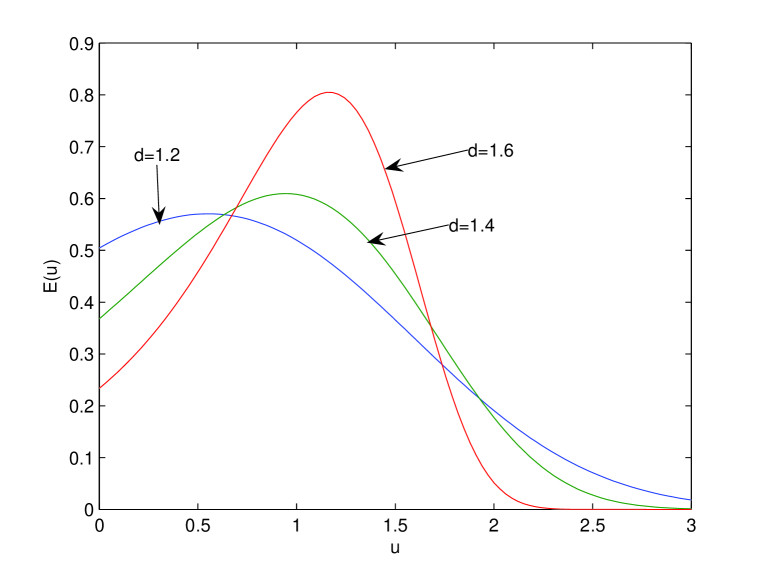
Figure 11: Plots of the distribution $\mathcal{E}(u)$ given by (148) for $d=1.2;1.4;1.6$.

Fig. 11 plots the PDF $\mathcal{E}(u)$ given by (148) for different values of the fractal dimension $d$ of the set of earthquake epicenters. The tail of $\mathcal{E}(u)$ is more extended for smaller fractal dimensions $d$.

The explicit form (147) of $\mathcal{E}(u)$ allows us to obtain the Laplace transforms $\hat{\mathcal{E}}(x)$ defined by (118) as

$$\hat{\mathcal{E}}(x)=E_{d/2}(-\bar{u}x)~{},$$ (149)

where $E_{g}(z)$ is the Mittag-Leffler function which has the following integral representation

$$E_{g}(-v)={v\over\pi}\sin(\pi g)\int_{0}^{\infty}{y^{g-1}e^{-y}dy\over v^{2}+y^{2g}+2vy^{g}\cos(\pi g)}~{}.$$ (150)

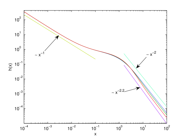
Figure 12: Plots of the PDF $h(x)$ of inter-event times given by (117) corresponding to the PDF (147) of the average regional seismic rates. Top to bottom on the right side of the picture $d=1.2;1.4;1.6$. The straight lines show asymptotic power laws, as proposed by Bak et al. (2002).

We then calculate explicitely the corresponding PDF $h(x)$ given by (117) of the inter-event times associated with (147). The results are shown in Fig. 12 for three different values $d=1.2,1.4,1.6$ of the fractal dimension of earthquake epicenters.

Fig. 13 is the culmination of the present work. It first makes use of our theoretical analysis based on the ETAS model leading to the prediction (108) for a single homogeneous seismc region, which is combined for multiple regions with different seismic rates distributed according to the PDF (147) predicted from our fractal model of earthquake epicenters, to finally obtain the global PDF (117) of inter-event times. Our final prediction (117) is compared to the empirical distribution represented in Fig. 2 of (Corral, 2004a), for the parameters $d=1.8$, $n=0.9$, $\gamma=1,1$ and to 3 values of the magnitude threshold $m-m_{0}=2;4;6$. The agreement is remarkable.

7 Concluding remarks

We have proposed a general theoretical approach to describe the statistics of recurrence times between successive earthquakes in a given region, or averaged over multiple regions. This work was motivated by the reports by several authors that recurrence times between successive earthquakes should be considered for broad areas, rather than for individual faults, and could provide important insights in the physical mechanisms of earthquakes. Several authors mainly from the Physics literature have proposed that the scaling law (1) found to describe well empirical data reveals a complex spatio-temporal organization of seismicity, which can be viewed as an intermittent flow of energy released within a self-organized (perhaps critical) system, for which concepts and tools from the theory of critical phenomena can be applied.

We have shown that this view is probably too romantic because much simpler explanations can be proposed to fully account for the empirical observations. Indeed, we have shown that the so-called universal scaling laws of inter-event times do not reveal more information than what is already captured by the well-known laws of seismicity (Gutenberg-Richter and Omori, essentially), together with the assumption that all earthquakes are similar (no distinction between foreshocks, mainshocks and aftershocks). This conclusion is reached by a combination of analyses, which start from a generalization of Molchan (2005)’s argument, to go to simple models of triggered seismicity taking into account Omori’s law, and end with a detailled study of what the ETAS model has to tell us on the statistics of inter-event times. By using the formalism of generating probability functions, we have been able to derive analytically specific predictions for the PDF of recurrence times between earthquakes in a single homogeneous region as well as for multiple regions. Our theory has been found to account quantitatively precisely for the empirical power laws found by Bak et al. (2002) and Corral (2003; 2004a). We showed in particular that the empirical statistics of inter-event times result from subtle cross-overs rather than being genuine asymptotic scaling laws. We also showed that universality does not strictly hold.

Therefore, to the question raised in the introduction, we are led to conclude that the statistics on inter-event times described in (Bak et al., 2002; Corral, 2003, 2004a,b, 2005a; Livina et al., 2005) is not really new in the sense that they do not reveal information which is not already contained in the known laws of seismicity. Our conclusion is that they can be derived from the known statistical properties of seismicity, so that they are only different ways of presenting the same information. In particular, the fact that the simple models of Lindman et al. (2005) are not able to fully reproduce the structure of the empirical statistics of recurrence times, as noted by Corral and Christensen (2006), does not necessarily imply that the so-called “unified scaling laws” reveal any novel information. We think we have clearly shown that they can be derived from simple and well-known physical ingredients, when carefully taking into account the physics of triggering between earthquakes. In this sense, the present work is the continuation of an effort to classify the empirical observations which can be, from those which cannot be, explained by the simple ETAS benchmark (Helmstetter and Sornette, 2003a; 2003b; Saichev and Sornette, 2005; 2006a). With this effort, we hope to eventually help identify real robust statistics which can not be explained by the ETAS benchmark or its siblings, leading us towards the acquisation of new interesting and important knowledge on the physics of earthquakes with potential applications for their forecasts.

References

Bak, P., K. Christensen, L. Danon, and T. Scanlon (2002), Unified Scaling Law for Earthquakes, Phys. Rev. Lett. 88, 178501.

Christensen, K., L. Danon, T. Scanlon, and P. Bak (2002), Unified Scaling Law for Earthquakes Proc. Natl. Acad. Sci. USA 99, 2509-2513 (2002).

Console, R., A.M. Lombardi, M. Murru, D. Rhoades (2003a), Bath’s law and the self-similarity of earthquakes, J. Geoph. Res., 108, 2128-2136, doi:10.1029/2001JB001651.

Console, R. and Murru, M., (2001), A simple and testable model for earthquake clustering, J. Geophys. Res. 106, 8699-8711.

Console R., Murru, M., Lombardi, A.M., (2003b), Refining earthquake clustering models, J. Geophys. Res. 108, 2468, doi:10.1029/2002JB002130.

Console, R., M Murru, and F. Catalli (2006), Physical and stochastic models of earthquake clustering, Tectonophysics 417, 141-153

Console, R., D. Pantosti, G. D’Addezio (2002), Probabilistic approach to earthquake prediction, Ann. Geophysics, 45 (6), 723-731.

Corral, A. (2003), Local distributions and rate fluctuations in a unified scaling law for earthquakes, Phys. Rev. E 68, 035102(R).

Corral, A. (2004a), Universal local versus unified global scaling laws in the statistics of seismicity, Physica A, 340, 590-597.

Corral, A. (2004b), Long-term clustering, scaling, and universality in the temporal occurrence of earthquakes, Phys. Rev. Lett. 92, 108501.

Corral, A. (2005a), Mixing of rescaled data and Bayesian inference for earthquake recurrence times, Nonlinear Processes in Geophysics 12, 89-100 (2005).

Corral, A. (2005b), Renormalization-Group Transformations and Correlations of Seismicity, Phys. Rev. Lett. 95, 028501.

Corral, A. and K. Christensen (2006), Comment on “Earthquakes Descaled: On Waiting Time Distributions and Scaling Laws,” Phys. Rev. Lett. 96, 109801.

Daley, D.J. and D. Vere-Jones (1988), An Introduction to the Theory of Point Processes, New York, Berlin: Springer-Verlag.

Davy, P., A. Sornette and D. Sornette (1990), Some consequences of a proposed fractal nature of continental faulting, Nature 348, 56-58.

Gerstenberger, M.C., S. Wiemer, L.M. Jones and P.A. Reasenberg, (2005), Real-time forecasts of tomorrow’s earthquakes in California, Nature 435 (7040), 328-331.

Global Earthquake Satellite System – A 20 year plan to enable earthquake prediction (2003), NASA and JPL, JPL 400-1069 03/03.

Gnedenko, B.V. and A. N. Kolmogorov (1954), Limit Distributions for Sums of Independent Random Variables (Addison-Wesley).

Hawkes, A.G. and D. Oakes (1974), A cluster representation of a self-excited point process, J. Appl. Prob. 11, 493-503.

Helmstetter, A., Y. Kagan and D. Jackson (2005), Importance of small earthquakes for stress transfers and earthquake triggering, J. Geophys. Res., 110, B05S08, 10.1029/2004JB003286.

Helmstetter, A. and D. Sornette (2002), Sub-critical and supercritical regimes in epidemic models of earthquake aftershocks, J. Geophys. Res. 107, NO. B10, 2237, doi:10.1029/2001JB001580.

Helmstetter, A. and D. Sornette (2003a), Foreshocks explained by cascades of triggered seismicity, J. Geophys. Res. (Solid Earth) 108 (B10), 2457 10.1029/2003JB002409 01.

Helmstetter, A. and D. Sornette (2003b) Bath’s law Derived from the Gutenberg-Richter law and from Aftershock Properties, Geophys. Res. Lett., 30, 2069, 10.1029/2003GL018186.

Helmstetter, A. and D. Sornette (2003c) Importance of direct and indirect triggered seismicity in the ETAS model of seismicity, Geophys. Res. Lett. 30 (11) doi:10.1029/2003GL017670.

Helmstetter, A., D. Sornette and J.-R. Grasso (2003), Mainshocks are Aftershocks of Conditional Foreshocks: How do foreshock statistical properties emerge from aftershock laws, J. Geophys. Res., 108 (B10), 2046, doi:10.1029/2002JB001991.

Jones, L. M., R. Console, F. Di Luccio and M. Murru (1999) Are foreshocks mainshocks whose aftershocks happen to be big? preprint available at http://pasadena.wr.usgs.gov/office/jones/italy-bssa.html

Kagan, Y.Y. and L. Knopoff (1980), Spatial distribution of earthquakes: The two-point correlation function, Geophys. J. Roy. Astr. Soc., 62, 303-320.

Kagan, Y.Y. and L. Knopoff (1981) Stochastic synthesis of earthquake catalogs, J. Geophys. Res., 86, 2853-2862

Knopoff, L., Y.Y. Kagan and R. Knopoff (1982), earthquakes sequences, Bull. Seism. Soc. Am. 72, 1663-1676.

Kossobokov, V.G. and S.A. Mazhkenov (1988), Spatial characteristics of similarity for earthquake sequences: Fractality of seismicity, Lecture Notes of the Workshop on Global Geophysical Informatics with Applications to Research in Earthquake Prediction and Reduction of Seismic Risk (15 Nov.-16 Dec., 1988), ICTP, 1988, Trieste, 15 p.

Lee, M.W., D. Sornette and L. Knopoff (1999), Persistence and Quiescence of Seismicity on Fault Systems, Phys. Rev. Lett. 83, 4219-4222.

Lindman, M., K. Jonsdottir, R. Roberts, B. Lund, and R. Bödvarsson (2005), Earthquakes descaled: On waiting time distributions and scaling laws, Phys. Rev. Lett. 94, 108501.

Livina, V.N., S. Havlin, and A. Bunde (2005), Memory in the occurrence of earthquakes, Phys. Rev. Lett. 95, 208501.

Metzler, R. and J. Klafter (2000), The random walk’s guide to anomalous diffusion: a fractional dynamics approach, Physics Reports 339, 1-77

Molchan, G.M. (2005), Interevent time distribution of seismicity: a theoretical approach, Pure appl. geophys., 162, 1135-1150.

Molchan, G. and T. Kronrod (2005), Seismic Interevent Time: A Spatial Scaling and Multifractality, preprint physics/0512264 (2005).

Ogata, Y. (1988), Statistical models for earthquake occurrences and residual analysis for point processes, J. Am. Stat. Assn. 83, 9-27.

Ogata, Y. (2005), Detection of anomalous seismicity as a stress change sensor, J. Geophys. Res., Vol.110, No.B5, B05S06, doi:10.1029/2004JB003245.

Ogata Y. and Zhuang J. (2006), Space–time ETAS models and an improved extension, Tectonophysics. 413 (1-2), 13-23.

Ouillon, G., C. Castaing and D. Sornette (1996), Hierarchical scaling of faulting, J. Geophys. Res. 101, B3, 5477-5487.

Reasenberg, P. A. and Jones, L. M. (1989), Earthquake hazard after a mainshock in California, Science 243, 1173-1176.

Reasenberg, P. A. and Jones, L. M. (1994), Earthquake aftershocks: Update, Science 265, 1251-1252 (1994)

Saichev, A. and D. Sornette (2005), Distribution of the Largest Aftershocks in Branching Models of Triggered Seismicity: Theory of the Universal Bath’s law, Phys. Rev. E 71, 056127.

Saichev, A. and D. Sornette (2006a), Power law distribution of seismic rates: theory and data, Eur. J. Phys. B 49, 377-401.

Saichev, A. and D. Sornette (2006b), Renormalization of the ETAS branching model of triggered seismicity from total to observable seismicity, in press in Eur. Phys. J. B (http://arxiv.org/abs/physics/0507024)

Saichev, A. and D. Sornette (2006c) “Universal” Distribution of Inter-Earthquake Times Explained, submitted to Phys. Rev. Letts. (http://arxiv.org/abs/physics/0604018)

Schwartz, D. P. and K. J. Coppersmith (1984), Fault behavior and characteristic earthquakes: Examples from the Wasatch and San Andreas fault zones, J. Geophys. Res., 89, 5681-5698.

Sieh, K.E. (1981), A review of geological evidence for recurrence times of large earthquakes, in Earthquake Prediction – An International Review, Maurice Ewing Series 4 (the American Geophysical Union).

Sornette, A. and D. Sornette (1999), Renormalization of earthquake aftershocks, Geophys. Res. Lett. 6, N13, 1981-1984.

Sornette, D. (2004), Critical Phenomena in Natural Sciences, Chaos, Fractals, Self-organization and Disorder: Concepts and Tools, 2nd ed. (Springer Series in Synergetics, Heidelberg).

Sornette, D. and M.J. Werner (2005a), Constraints on the Size of the Smallest Triggering Earthquake from the ETAS Model, Baath’s Law, and Observed Aftershock Sequences, J. Geophys. Res. 110, No. B8, B08304, doi:10.1029/2004JB003535.

Sornette, D. and M.J. Werner (2005b), Apparent Clustering and Apparent Background Earthquakes Biased by Undetected Seismicity, J. Geophys. Res., Vol. 110, No. B9, B09303, 10.1029/2005JB003621,

Steacy, S., J. Gomberg and M. Cocco (2005), Introduction to special section: Stress transfer, earthquake triggering, and time-dependent seismic hazard, J. Geophys. Res. 110, B05S01, doi:10.1029/2005JB003692.

Utsu, T., Y. Ogata and S. Matsu’ura (1995), The centenary of the Omori Formula for a decay law of aftershock activity, J. Phys. Earth 43, 1-33.

Working Group on California Earthquake Probabilities (2003) Earthquake Probabilities in the San Francisco Bay Region: 2002-2031, Open-File Report 03-214, USGS.

Wyss, M., D. Schorlemmer, and S. Wiemer (2000), Mapping asperities by minima of local recurrence time: San Jacinto-Elsinore fault zones, J. Geophys. Res. 105 (B4), 7829-7844.

Zhuang J., Chang C.-P., Ogata Y. and Chen Y.-I. (2005), A study on the background and clustering seismicity in the Taiwan region by using a point process model, Journal of Geophysical Research, 110, B05S18, doi:10.1029/2004JB003157.

Zhuang J., Ogata Y. and Vere-Jones D. (2002), Stochastic declustering of space-time earthquake occurrences, Journal of the American Statistical Association, 97, 369-380.

Zhuang J., Ogata Y. and Vere-Jones D. (2004), Analyzing earthquake clustering features by using stochastic reconstruction, Journal of Geophysical Research, 109, No. B5, B05301, doi:10.1029/2003JB002879.

Figure 5: Dependence on $m$ of the parameter $\delta$ defined in (86), which results from the competition between the GR and productivity laws. Bottom to top: $\gamma=1.1;1.2;1.3$.

Figure 13: Plots of the empirical PDF of inter-event times in multiple regions collected in Fig. 2 of (Corral, 2004a), which is compared with our theoretical PDF $h(x)$ given by (117) (thick lines), represented for the parameters $d=1.8$, $n=0.9$, $\gamma=1,1$ and three values of the threshold magnitude $m-m_{0}=2;4;6$. Corral calculated the recurrence-time probability densities following Bak et al. (2002)’s procedure, after rescaling by the regional seismic rates. 84 distributions are shown, with region sizes $L$ ranging from $0.039^{\circ}$ to $45^{\circ}$, and threshold magnitudes $m$ varying between $1.5$ and $6$. The curves are shifted by factors $1;10^{-2};10^{-4}$ and $10^{-6}$, and correspond to: 1 (top), Southern California, 1984-2001; 2, Northern California, 1985-2003; 3, Southern California, 1988-1991 (stationary rate), NEIC, 1973-2002, Japan, 1995-1998, and Spain, 1993-1997; 4 (bottom), New Zealand, 1996-2001, and New Madrid, 1975-2002. The thin straight lines are Corral’s fits by power laws of the short or intermediate times: 1 (top), $0.12/x^{0.95}$; 2, $0.15/x^{0.9}$, 3 and 4 (bottom), $0.05/x^{0.95}$ and $0.5/x^{0.5}$. In all cases, Corral has fitted the long-time tail by $0.25/x^{2.2}$. The times in the horizontal axis span from 2 min to about 20 years. Recurrence times smaller than 4, 10, and 2 min are not shown, for Japan, NEIC, and the rest of catalogs, respectively.