AMPLIFICATION AND INCREASED DURATION OF EARTHQUAKE MOTION ON UNEVEN STRESS-FREE GROUND
Armand WIRGIN1, Jean-Philippe GROBY2
1
Laboratoire de Mécanique et d’Acoustique, UPR 7051 du CNRS,
Marseille, France.
2 Laboratorium v. Akoestiek en Thermische
Fysica, Katholieke Universiteit, Leuven, Belgium.
ABSTRACT- When a flat stress-free surface (i.e., the ground
in seismological applications) separating air from a isotropic,
homogeneous or horizontally-layered, solid substratum is solicited
by a SH plane body wave incident in the substratum, the response
in the substratum is a single specularly-reflected body wave. When
the stress-free condition, equivalent to vanishing surface
impedance, is relaxed by the introduction of a spatially-
constant, non- vanishing surface impedance, the response in the
substratum is again a single reflected body wave whose amplitude
is less than the one in the situation of a stress-free ground.
When the stress-free condition is relaxed by the introduction of a
a spatially-modulated surface impedance,
which simulates the action of an
uneven (i.e., not entirely-flat) ground , the frequency-domain
response takes the form of a spectrum of plane body waves and
surface waves and resonances are produced at the frequencies
of which one or several surface wave amplitudes can become large.
It is shown, that at resonance, the amplitude of one, or of
several, components of the motion on the surface can be amplified
with respect to the situation in which the surface impedance is
either constant or vanishes. Also, when the solicitation is
pulse-like, the integrated time history of the square of surface
displacement and of the square of velocity can be larger, and the
duration of the signal can be considerably longer, for a
spatially-modulated impedance surface than for a constant, or
vanishing, impedance surface.
1 Introduction
An important question in seismology, civil engineering, urban planning, and natural disaster risk assessment is: to what extent does surface topography of different length and height scales (ranging from those of mountains and hills to city blocks and buildings) modify the seismic response (in terms of cumulative motion intensity and duration) on the ground?
There exists experimental evidence (Singh and Ordaz, 1993; Davis and West, 1973; Griffiths and Bollinger, 1979) that this modification is real and can attain considerable proportions.
Some theoretical studies (Wirgin, 1989; Wirgin 1990; Wirgin and Kouoh-Bille, 1993; Groby, 2005) seem to indicate that such effects are indeed possible, but various numerical studies ( Bouchon, 1973; Bard, 1982; Sanchez-Sesma, 1987, Geli et al., 1988; Wirgin and Bard, 1996; Guéguen, 2000; Clouteau and Aubry, 2001; Guéguen et al., 2002; Semblat et al., 2003; Tsogka and Wirgin, 2003; Boutin and Roussillon, 2004; Kham, 2004; Groby and Tsogka, 2005) yield conflicting results in that some of these point to amplification, while others to very weak effects, or even to de-amplification. Contradictory results are also obtained regarding the duration of the earthquakes.
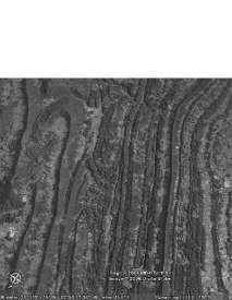
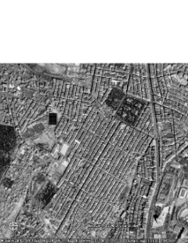
1.1 Sites
In figs. 1 and 2 we give examples of natural and man-made sites respectively with quasi-periodic features that can be studied by the methods of this investigation.
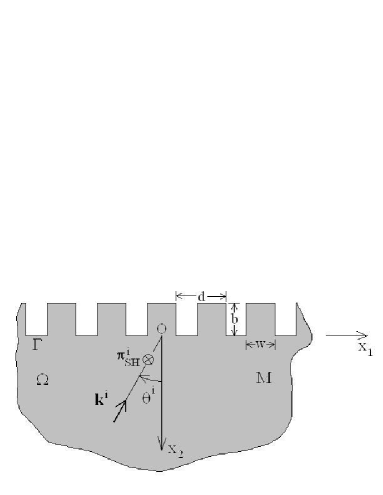
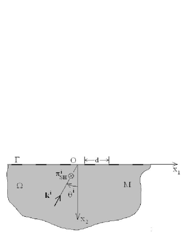
1.2 Physical configurations
1.3 On the notion of impedance
We shall employ the notion of (surface) impedance employed in the civil engineering (Guéguen, 2000), (Roussillon, 2006) community wherein the three components of impedance are which designate mass, stiffness and damping ( real constants) respectively.
Thus, the mechanical impedance is complex and designated by , where is the ”resistive” part, and the ”reactive” part.
The reactance is ”inductive” if (i.e., ) and is ”capacitive” if (i.e., .
2 Governing equations
2.1 Mathematical translation of the boundary value problem in the space-frequency domain
| (1) |
| (2) |
| (3) |
| (4) |
wherein: is the total displacement field, the (unknown) diffracted field, the (known) incident field , the angle of incidence with respect to the axis, the incident pulse spectrum.
| (5) |
When the impedance vanishes for all , the boundary condition becomes that of a flat, stress-free surface.
Otherwise, the impedance boundary condition is supposed to simulate the presence of a topo-graphically- uneven stress-free surface.
The periodic nature of is expressed by:
| (6) |
| (7) |
It is also assumed that , i.e., the impedance is passive and dissipative.
2.2 Diffracted field representation
| (8) |
| (9) |
The diffracted field is a discrete sum of plane waves: those for which is real are propagative (or homogeneous) and those for which is imaginary are evanescent or (inhomogeneous).
2.3 Result of the introduction of the field representation into the boundary condition
| (10) |
wherein
| (11) |
The linear system can be written as the infinite-order matrix equation
| (12) |
3 On the possibility of anomalous fields in the general case of a periodic, passive, spatially non-constant, surface impedance
A mode of the configuration is obtained by turning off the solicitation in the matrix equation, i.e., , wherein is the null vector.
We are thus faced with the equation , whose solution is trivial (i.e., ), unless
| (13) |
An ”eigenvalue” is a value of for which the determinant vanishes at a given frequency. Another way of putting things is to fix and look for the frequencies (”natural frequencies”) that lead to a vanishing determinant.
When the configuration is such that one of the is an eigenvalue, and the frequency is a natural frequency, then the system is said to be in a state of resonance.
When this happens, the determinant of is either small or nil, which means that the inverse of is either large or infinite and that consequently one or more entries in the vector of the scattered plane wave coefficients are either large or infinite.
Consequently, we can expect (since the field is a discrete sum of scattered plane waves) that the field may become large at resonance (in the presence of not too much dissipation and/or radiation damping).
From now on, we call det the general dispersion relation. In the case of spatially-constant surface impedance , only the zeroth-order diffracted wave is generated, so that the dispersion relation is
| (14) |
and the latter has no solution for a passive impedance (i.e., ) due to the fact that is real.
This means that no resonance can be produced for a constant, passive impedance surface. When the surface impedance function Z is not spatially-constant, it is much more difficult to obtain a meaningful expression of the dispersion relation.
Some insight may be gained by turning to an iteration method of solution
| (15) |
which suggests that can become large for
| (16) |
This cannot occur for for the previously-mentioned reason. It can occur, if at all, only for . Recall that it was assumed that =0, and
| (17) |
Consider the case of vanishing resistance, i.e., in which the approximate dispersion relation is
| (18) |
Since , , , and , the second term in the previous equation is either positive real (for real ) or positive imaginary (for imaginary ), so that the sum of the two terms can vanish only if
| (19) |
The first of these requirements means that the impedance must be inductive for it to be possible to obtain resonant behavior. Thus, a possible explanation of why several researchers, who employed the impedance concept to account for ground uneveness, have not been able to obtain anomalous fields is that their impedance functions were such that in the frequency range of the incident pulse. The second requirement, i.e., , means that resonances can occur only for the evanescent waves in the plane wave representation of the scattered field. Thus, we can expect the amplitude of the -th order evanescent wave to become infinite (for ) or large (for ) at resonance, which is another way of saying that a surface wave (evanescent waves are of this sort) is strongly excited at resonance (all the more so the smaller is ).
This picture is only partially true, because the approximate dispersion relation may account only poorly for all the features of the solutions of the general dispersion relation, which is the case if the uneveness of the ground is large.
The fact that becomes large at resonance is a necessary condition for the ground motion to be large at this resonance frequency, but is not a sufficient condition due to the fact that the diffracted field is composed not of one evanescent plane wave, but of a sum of both propagative and evanescent plane waves, and this sum can be of modest proportions even when one of its components is large. Such modest fields at resonance are due mainly to radiation damping.
3.1 The case of spatially- sinusoidal surface impedance
For the computations, wee shall choose:
| (20) |
When , we re-encounter the case of a constant impedance on flat ground, so that is a measure of the uneveness of the ground.
4 Computations
We shall be interested in the following quantities indicative of possible anomalous effects provoked by the uneveness of the ground:
-
•
the duration of significative seismic ground motion,
-
•
the peak value of the ground displacement,
-
•
the amplification factors (i.e., amplification if the factor , de-amplification if the factor ) of the time integral (over ) of the squared displacement (velocity v) for the modulated impedance surface relative to the time integral (over ) of squared displacement (velocity) for the impedance surface:
(21) -
•
the amplification factors of the time integral (over )of squared displacement (velocity) for the modulated impedance surface relative to the time integral (over ) of squared displacement (velocity) for the stress-free surface:
(22)
The amplitude spectrum of the incident plane wave is that of a Ricker pulse, i.e., .
The other parameters are: , , , , , , .
The results of the computations, peformed by direct resolution of a suitably-chosen finite dimension version of the matrix equation, are given in figs. 5 and 6 for and respectively. The first line in these figures contains the spectra, the second line the time histories, and the remaining lines the ratios of cumulative response.
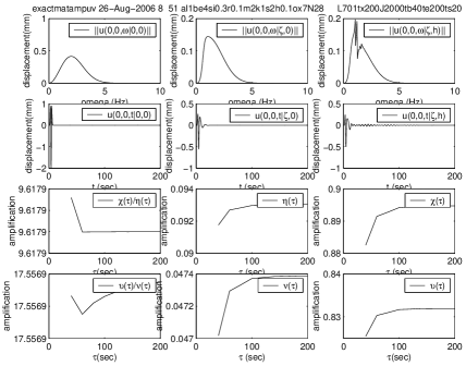
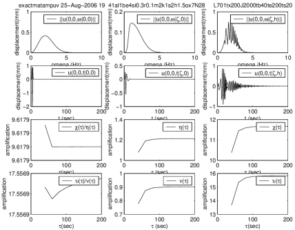
5 Comments
The spectra reveal the existence of a series of resonances, as predicted by the theory.
The peak displacement (in the time domain) on a spatially-modulated impedance ground is always smaller than the peak displacement on the flat, stress-free ground.
The maximum values of the ratios , , and first increase and then decrease with increasing , with the maximum amplifications (, , , ) being attained for .
It is possible to obtain substantial amplification of the ratios with respect to the spatially-constant impedance flat surface and much less amplification or even deamplification of the ratios with respect to the stress-free flat surface.
This shows that although there is no doubt that spatially-modulated impedance surfaces can give rise to beating and very long durations, attaining in some of these examples of the order of 2 min versus of the order of 10-20 sec for zero or non-zero constant impedances), there is no clear-cut answer to the question of whether spatial impedance modulations, which simulate the existence of ground uneveness, systematically result in amplification or even deamplification of cumulative ground motion displacement and velocity, especially with respect to motion of a stress-free flat ground.
References
- [1] P.-Y. Bard. Diffracted waves and displacement field over two-dimensional elevated topographies. Geophys.J.R.Astron.Soc., 71:731–760, 1982.
- [2] M. Bouchon. Effect of topography on surface motion. Bull.Seism.Soc.Am., 63:615–632, 1973.
- [3] C. Boutin C. and P. Roussillon. Assessment of the urbanization effect on seismic response. Bull.Seism.Soc.Am., 94:251–268, 2004.
- [4] D. D. Clouteau and D. Aubry. Modifications of the ground motion in dense urban areas. J.Comput.Acoust., 9:1659–1675, 2001.
- [5] L.L. Davis and L.R. West. Observed effects of topography on ground motion. Bull.Seism.Soc.Am., 63:283–298, 1979.
- [6] L. Geli, P.-Y. Bard, and B. Jullien. The effect of topography on earthquake ground motion: a review and new results. Bull.Seism.Soc.Am., 78:42–63, 1988.
- [7] D.W. Griffiths and G.A. Bollinger. The effect of the Appalachian mountain topography on seismic waves. Bull.Seism.Soc.Am., 69:1081–1105, 1979.
- [8] J.-P. Groby. Modélisation de la propagation des ondes élastiques générées par un séisme proche ou éloigné à l’intérieur d’une ville. PhD thesis, Université de la Méditerranée, Marseille, 2005.
- [9] J.-P. Groby, C. Tsogka, and A. Wirgin. Simulation of seismic response in a city-like environment. Soil Dynam.Earthquake Engrg., 25:487–504, 2005.
- [10] P. Gueguen. Interaction sismique entre le sol et le bâti: de l’interaction sol-structure à l’interaction site-ville. PhD thesis, Université Joseph Fourier, Grenoble, 2000.
- [11] P. Gueguen, P.-Y. Bard, and F.J. Chavez-Garcia. Site-city seismic interaction in Mexico city like environments : an analytic study. Bull.Seism.Soc.Am., 92:794–804, 2002.
- [12] M. Kham. Propagation d’ondes sismiques dans les bassins sédimentaires: des effets de site à l’interaction site-ville. PhD thesis, Laboratoire Central des Ponts et Chaussées, Paris, 2004.
- [13] P. Roussillon. Interaction sol-structure et interaction site-ville: aspects fondamentaux et modélisation. PhD thesis, Institut National des Sciences Appliquées de Lyon, 2006.
- [14] F.J. Sanchez-Sesma. Site effects on strong ground motion. Soil Dynam.Earthqu.Engrg., 6:124–132, 1987.
- [15] J.F. Semblat, P. Guéguen, M. Kham, P.-Y. Bard, and A.-M. Duval. Site-city interaction at local and global scales. In 12th European Conference on Earthquake Engineering, Oxford, 2003. Elsevier. paper no. 807 on CD-ROM.
- [16] S.K. Singh and M. Ordaz. On the origin of long coda observed in the lake-bed strong-motion records of Mexico City. Bull.Seism.Soc.Am., 83:1298–1306, 1993.
- [17] C. Tsogka and A. Wirgin. Simulation of seismic response in an idealized city. Soil. Dynam.Earthquake Engrg., 23:391–402, 2003.
- [18] A. Wirgin. Amplification résonante du tremblement d’une chaîne de montagnes cylindriques soumise à une onde SH. C.R.Acad.Sci. Paris II, 311:651–655, 1989.
- [19] A. Wirgin. Amplification résonante du mouvement du sol sur une montagne cylindrique isolée soumise à une onde sismique SH. C.R.Acad.Sci. II, 311:651–655, 1990.
- [20] A. Wirgin and P.-Y. Bard. Effects of buildings on the duration and amplitude of ground motion in mexico city. Bull.Seism.Soc.Am., 86:914–920, 1996.
- [21] A. Wirgin and L. Kouoh-Bille. Amplification du mouvement du sol au voisinage d’un groupe de montagnes de profil rectangulaire ou triangulaire soumis à une onde sismique SH. In Génie Parasismique et Aspects Vibratoires dans le Génie Civil, pages ES28–ES37, Saint-Rémy- lès-Chevreuse, 1993. AFPS.