Microeconomic co-evolution model for financial technical analysis signals

Abstract

Technical analysis (TA) has been used for a long time before the availability of more sophisticated instruments for financial forecasting in order to suggest decisions on the basis of the occurrence of data patterns. Many mathematical and statistical tools for quantitative analysis of financial markets have experienced a fast and wide growth and have the power for overcoming classical technical analysis methods. This paper aims to give a measure of the reliability of some information used in TA by exploring the probability of their occurrence within a particular $microeconomic$ agent based model of markets, i.e., the co-evolution Bak-Sneppen model originally invented for describing species population evolutions. After having proved the practical interest of such a model in describing financial index so called avalanches, in the prebursting bubble time rise, the attention focuses on the occurrence of trend line detection crossing of meaningful barriers, those that give rise to some usual technical analysis strategies. The case of the NASDAQ crash of April 2000 serves as an illustration.

Key words SOC model, Technical analysis, large financial crashes.
PACS 01.75.+m Science and society - 89.90.+n Other areas of general interest to physicist

1 Introduction

Quantitative analysis of financial market data has well assessed several properties like the long term memory in volatility [1, 2, 3, 4], returns [5, 6, 7], speculative bubbles [8], and the presence of fractals [9] that has been extensively studied since a pioneering paper [10]. Many mathematical and statistical models [11, 12, 13, 14, 15, 16] are available nowadays for a phenomenological description of financial data, while rigorous theoretical frameworks have shown to be able to encapsulate some conjectures like the Elliot waves [17].

Alongside the descriptive analysis of macroeconomic quantities, theories derived for complex systems can explain the aggregate behavior of markets through the analysis of its components at the microeconomic level. Microeconomic models of financial markets rank in complexity from the simplest models, typically considering the interaction of two main types of agents - the fundamentalists and the chartists [18, 19, 20, 21]- to the most heterogeneous types of agents; an intermediate step considering the presence of noise traders that act either without market information or not caring about the fundamentals, thus creating white noise, while mean reversion effects [22] can be accounted due to the activity of fundamentalists. The first question to be raised is whether a microeconomic approach can be found based on insight about the mechanism of the formation of financial quantities. If investigations of micro- or macro-economic models rely on simulation frameworks whenever more theoretical tools are not available, the evaluation of investment strategies driven by models, even empirical ones, like those leading to technical analysis (TA) is a need. Nevertheless it is difficult to implement them, even through simulations of multi agent systems, because of the lack of reliability of the parameters. Indeed it is not easy to perform computer simulations of markets with interacting agents that trigger their orders on the basis of technical analysis patterns because technical analysis rules are more complex than those commonly assigned to chartists and fundamentalists in computer simulations. Moreover, to get the best trading decision is still an art, independently from a model sophistication; indeed the interpretation of charts heavily relies on the expertise of the analyst.

Therefore we study model property and statistics instead of trying to draw results relying on heavy computer simulations of a multi agent system.

On the other hand, a decision based on financial signal technical analysis must take into account the temporary occurrence of several patterns. However to start the study of the occurrence and of the reliability of the simplest components is a compulsory step towards the comprehension of more complex configurations. This can in turn lead to a systematic assessment of the expertise of such a kind of market analysts.

A cornerstone for technical analysis comes from the expertise of Charles H. Dow that developed the set of methods that are gathered under the name of Dow theory. Dow theory [23] considers major trends as those lasting more than one year. Intermediate trends are those that range from a minimum of three weeks to a maximum of several months, as those which can be useful in futures markets. Short trends can be identified for time intervals shorter than two or three weeks. Thus it is very important to decide upon a reliable time interval for implementing a strategy, before trying to define any trend. Statistics of trend lines will be exploited on the aggregate of the proposed microeconomic model and compared with the results obtained on raw data. Such analyzes should show their power at their best when performed during periods of high risk exposure. Among them the rising part of speculative bubbles of market indices, due to endogenous causes, has been chosen here below because of the availability of already well assessed theories [24, 25, 26, 27, 28]. It is worth remarking that stock market indices actually are a weighted mean of stock prices. To perform buy/sell strategies on stock market indices (eventually triggered by TA signals) has the meaning to buy/sell a previous selected financial product replica of the index (Exchange Traded Funds (ETF), certificates).

Therefore the aim of this paper is twofold. The first task is to set up a microeconomic approach based on insight about the mechanism of the formation of financial quantities; the second target is to show how to use the property of the aggregate rising from the model structure in order to evaluate the reliability of already often used methods like those found by chartists in so called technical analysis (TA) [29]. In particular the analysis will focus on the probability estimate of the occurrence of trend lines slopes and on the estimate the probability of trend lines crossing.

The paper is organized as follows. The next section shortly gives an overview of the main properties of the NASDAQ July 2000 crash, of its statistical properties, and shows the bases of the models that we are going to apply and how to combine them for data modeling. Sec. 3 introduces TA signals of interest, in particular so called barriers. Sec. 4 shows how to use the model information in order to set up a tool in order to estimate both the occurrence of barrier crossing and the formation of a trend line.

Sec. 5 serves as a conclusion and suggestions for going beyond the present work. It will appear that the numerical values used to build the agent-based model describing the financial index are those of the $2$-dimensional square lattice Bak-Sneppen coevolution model [30]. For completeness the $1$-dimensional case is treated in an Appendix.

2 Microeconomic model

This section aims to set up a model for the rising part of speculative bubbles due to endogenous causes in order to capture data features as the property of long term memory, the distribution of the size of fluctuations around at the mean, and the main trend. The modelization tasks can be accomplished through several models, depending on the properties of the time series that need to be maintained. Already existing models for speculative bubbles [24, 25, 26, 27, 28] do provide a deterministic function for the main trend and oscillation modeling through log-periodic patters, but they don’t capture some residual correlation. Let them be improved as below.

2.1 Large financial crashes

The theory of speculative bubbles due to endogenous causes has been extensively examined indicating self similarity in market indices. Widely developed numerical studies have extracted common features of bubbles providing a range for the most important parameters, taxonomy of bubbles and investigation about signatures for bubbles due to endogenous causes [31]. Anytime the amplitude of the crash is proportional to the total price then there is a strong indication for modeling the logarithm of the index value [26, 32, 33], instead of using the index itself [31, 34].

The modelization of large financial crashes as critical points [25] and a subsequent simplification driven by universality assumptions [27, 28] lead to the approximation of the main trend of the logarithm of the stock market index w.r.t. the time to crash $t_{c}-t$ given by

$$F(t)=A+B\ln(t_{c}-t)$$ (1)

where $t_{c}$ is the most probable crash time and $A$, $B$ are parameters to be estimated via numerical optimization.

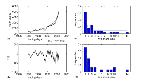
Figure 1: The NASDAQ 100 Composite index case study. (a) NASDAQ 100 Composite index daily closing value and its exponential approximating function (1). The data set used in order to study the ascending speculative bubble ending at the crash is for the trading days since January 1^st, 1997 till March 10^th, 2000, for a total of 833 points. The vertical line corresponds to December 23^th, 1998 and emphasizes the starting day of the period that is best suitable for the BS model. (b) Plot of the residuals $R(t)$, as from Eq. (2), i.e., the difference between the raw NASDAQ 100 Composite index daily closing value and its exponential approximation. The horizontal line corresponds to the level $R(1)$. (c) The estimate of $P(T)$ on the entire time series at level $R(1)$ according to (3) gives $H=0.42(0.06,0.77)$. (d) The estimate of $P(T)$ on data since December 23^th, 1998 till the end gives $H=0.58(0.12,1.04)$ at the level of the first day value.

In order to show an example and for further reference below let us sum up the (speculative) bubble of the NASDAQ that collapsed into the crash of April 2000 (Fig. 1).

Accordingly to [26, 31] let the financial signal data $\{y(t)\}_{t=1,T}$ be the logarithm transformation of the NASDAQ 100 Composite index daily closing value between Jan. 01, 1997 and March 10, 2000, i.e. $T=833$. The best fit of (1) to the ascending part of the bubble has been performed using the minimum least squares method. The results are $A=7.91$, $B=-0.54$, and $t_{c}$ corresponding to July 4^th, 2000 [31, 35]. Notice that the actual crash date, April $11^{th}$ approximately occurs three months before the $t_{c}$ estimated by the fit. We have noticed on other data as well that this is usually experienced when (1) is used.

Evolution models more complex than (1) can be considered for the description of the main oscillations [31], but the scaling of correlations changes only slightly. The periods that correspond to the rise and to the successive burst of a speculative bubble due to endogenous causes are characterized by several oscillations around the main trend [24, 36, 37, 38], as widely examined through the papers that assess the similarities of large financial crashes properties with earthquake phenomena [31] or sandpile avalanches on fractal structures [24, 39]. Although the importance of log periodic accelerating oscillations going close to the most probable crash time is deeply connected with the self similarity hypothesis, and discrete scale invariance, its validity is still debated, because the residual correlation evidences the role of residual noise, pointing to the limit of the theory and suggesting to look for other models for describing the major fluctuations.

Let the so called residuals $R(t)$ be defined through (see Fig. 1(b) for a display)

$$R(t)=\exp(y(t))-\exp(F(t)).$$ (2)

It is usually found that most market index data $R(t)$ show long term memory correlation indicating a mean reverting process [22]. This implies that a useful statistical property to compare models to real data should be found in the Hurst exponent. The Detrended Fluctuation Analysis (DFA) technique [40, 41, 42] is often used in order to characterize fluctuation correlations in such time series, through the power law exponent $\alpha$. In this NASDAQ case study $\{R(t)\}_{t=1,T}$ is characterized by $\alpha=1.39(1.37,1.40)$ corresponding to a Hurst exponent $H\simeq 0.39(0.37,0.40)$. Thus the residuals $R(t)$ can be modeled through a theoretical fractional Brownian motion (fBm). In this case the time at which the random walker starting at the origin first returns to the origin, i.e. be the first return time $T$ of a fBm has the following probability decay [43, 44]:

$$P(T)\sim T^{H-2}.$$ (3)

The estimate of $P(T)$ on $\{R(t)\}_{t=1,T}$ data at the level of the initial time value $R(1)$ in the NASDAQ case gives $H=0.42(0.06,0.77)$ and fine agreement with the above estimated $H$ through the DFA (see Fig. 1(c)).

2.2 The Bak and Sneppen model

The simple Self-Organized Criticality model of Bak and Sneppen (BS) [30, 45, 46] has been shown to fulfill not only characteristics of species distribution evolutions like a power law in the distribution of avalanches, but also the characteristics required for earthquake modeling, both for spatial and temporal correlation functions, or also in landslides [47, 48, 49]. It is of great interest that the probability of the occurrence of the next avalanche can be estimated, as it emerges from the model dynamics. Interestingly earthquake models were shown to be well suited for the description of market data that are characterized by cascade crashes and are followed by slow recoveries [50, 27]. This behavior has been detected in several speculative bubbles and attributed to endogenous causes [8]. At each time $t$ the $d$-dimensional BS model deals with $L^{d}$ species that compete for their survival.

In a financial application of the BS model each species can represent either an agent or a class of them through a representative agent. At time $t$ each species is fully described by its fitness $f^{d}_{i}(t)$, $i=1,\cdots,L^{d}$ drawn at time $0$ from a uniform distribution in $[0,1]^{d}$. A change in fitness of one species implies an evolution of others as well: there is co-evolution. In the original evolution model the fitness can represent either the living capability of the species or the population, or a barrier to be overcome. The average fitness can be defined as the simple mean [51, 52, 53] of the individual fitness, i.e.,

$$\bar{f}^{d}(t)=\frac{1}{L^{d}}\sum_{i=1}^{L^{d}}f^{d}_{i}(t).$$

The BS model has been introduced for simulating the collective behavior of interacting groups or individuals. In financial markets each $f_{i}$ can be interpreted as the estimate of the market price by either groups or agents. On financial markets this mean fitness $\bar{f}^{d}(t)\in[0,1]$ can be used as an approximation of the market index value, resulting from the market price, as seen by/at each agent level, scaled to the $[0,1]$ interval as it is built up through the components of the market and the agent behaviors. Thus the $L^{d}$ species can be interpreted as $L^{d}$ groups of investors, more properly than just $L^{d}$ single investors, whose contribution to the formation of the price at time $t$ is given by $f^{d}_{i}(t)$ that can include the raw price $p^{d}_{i}(t)$ (normalized to $1$) as well as the raw price already multiplied by the weight of the group due to its social impact $f^{d}_{i}(t)=\omega^{d}_{i}(t)\,p^{d}_{i}(t)$, $\sum_{i}\omega^{d}_{i}(t)=1$.

Groups (agents in the smallest size case) are thus modeled as organized in a simple social lattice or network that in dimension $d$ connects each group only to his first $2d$ nearest neighbors. The usual boundary conventions of the Bak-Sneppen model hold. We are aware that this model should be considered as a high simplification of a social/financial network that keeps trace only of the most important influences of a group over the other. Extensions to more complex networks imply further work depending on possibly unrealistic features to be found in our $d$-dimensional model.

Let at each time step the group with the lowest price randomly ”adapt”, i.e., change the price and affect its nearest neighbors in the spirit of the BS model. Extremal values are those the furthest away from the mean. The replacement of the lowest value $f_{i}$ by a random number can be interpreted as the correction to the worst price underestimate. When $L\rightarrow\infty$, and for $t$ large enough almost all species have their fitness above a threshold $f^{d}_{c}$ [55, 56]; these fitnesses are therefore uniformly distributed in $(f^{d}_{c},1)$.

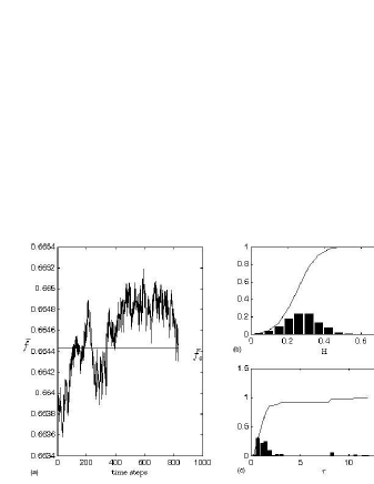
Figure 2: $2$-dimensional BS trajectory in the stable phase: (a) A sample and the critical level $\bar{f}_{c}$. For this sample $H=0.38(0.35,0.40)$, $\tau=0.05(-1.89,1.99)$. (b) Estimate of the self similarity degree $H$ through the DFA analysis on $1000$ trajectories of the $2$-dimensional BS model during the stable phase and its cumulative function. The mean is $0.277$ and the standard deviation is $\sigma_{H}=0.088$. The frequency of BS trajectories that have the $H$ exponent confidence interval overlapping the confidence interval of the NASDAQ $H$ on the entire time series is approximately $17\%$, while on the period since Dec. 23^th it is approximately $24\%$. (c) Estimate of the avalanche exponent $\tau$ on subsequences with length $T$ of trajectories of the $2$-dimensional BS model during the stable phase and its cumulative function. The mean is $1.9$ and the standard deviation is $\sigma_{\tau}=2.23$. The large $\tau$ spread around at the theoretical value $\tau=1.72$ can be addressed to finite-size of the sampling

An evaluation of the ”distance” of this simple toy model hypotheses and implications from true social/financial systems with complex interactions and imitative behaviors is nearly impossible. Nevertheless it is interesting to note that the threshold for $\bar{f}^{d}(t)$ becomes $\bar{f}^{1}_{c}=0.83351$ if $d=1$ and $\bar{f}^{2}_{c}=0.66443$ if $d=2$ [57] (Fig. 2(a)), as noticed by Li and Cai [52], reasonably similarly to what is found in some social systems. An interesting behavioral remark is that the critical threshold in the case $d=2$ fits social rules that assign a special weight to decisions when approximately $2/3$ of people agree.

2.3 Avalanches: degradation and recovery

At this stage it is of interest to stress that the BS model has led to several definitions of avalanches [30, 52, 55]. The duration of an avalanche in the original BS model refers to the time spent by the lowest $f_{i}(t)$ below $f_{c}$. On the other hand, Li and Cai define an avalanche (duration) as the time spent by $\bar{f}^{d}(t)$ below $\bar{f}^{d}_{c}$. This is in fact only degradation part of the whole BS avalanche. This definition neglects part of the signal, i.e. the time spent by the signal $\bar{f}^{d}(t)$ $above$ the threshold. This signal is of interest as well in particular in financial and social matters. One could define and analyze the statistics of time intervals between maxima (in/and minima) of the signal. These would encompass cycle like situations containing degradation $and$ recovery processes. In the present paper the Li-Cai avalanche definition will be used, leaving other definition investigation for other work.

An important feature concerns the structure of such avalanches. After the first transient phase the model dynamic leads to the activity of the system characterized by $\bar{f}^{d}(t)>\bar{f}^{d}_{c}$ [57]. Following the definition reported in [51, 52], the size $s$ of the degradation part of avalanches is defined as its temporal duration, i.e. an avalanche of size $s$ remains below $\bar{f}^{d}_{c}$ for $s-1$ time steps $\bar{f}^{d}(t)$. Thus the duration is the number $s$ such that

$$\bar{f}^{d}(t)>\bar{f}^{d}_{c},\bar{f}^{d}(t+1)<\bar{f}^{d}_{c},\cdots,\bar{f}^{d}(t+s-1)<\bar{f}^{d}_{c},\bar{f}^{d}(t+s)>\bar{f}^{d}_{c}.$$

It has been shown [57, 58] that the $s$-distribution of such degradation part of avalanches follows a power law

$$P(s)\propto s^{-\tau}.$$ (4)

For the $1$-dimensional BS model $\tau=1.8$; for the $2$-dimensional square lattice BS model $\tau=1.72$ [51]. Moreover although the average avalanche size depends on the distance from $\bar{f}^{d}_{c}$, the values of $\tau$ are independent of the level chosen [52] for an infinite system.

For the purposes of TA, and trend line property searches we also studied the recovery situation, identified by the permanence of the signal above the threshold $\bar{f}^{d}(t)$ in the sense of Li-Cai. In order to do so a mirror-like situation must be envisaged.

Of course $-\bar{f}^{d}(t)$ has the same long memory degree as $\bar{f}^{d}(t)$; moreover it is possible to define the recovery size $s$ as being a sequence of $s$ time steps such that

$$-\bar{f}^{d}(t)<-\bar{f}^{d}_{c},-\bar{f}^{d}(t+1)>-\bar{f}^{d}_{c},\cdots,-\bar{f}^{d}(t+s-1)>-\bar{f}^{d}_{c},-\bar{f}^{d}(t+s)<-\bar{f}^{d}_{c}.$$

Because of the fact that

$$P(-\bar{f}^{d}(t)<-\bar{f}^{d}_{c},-\bar{f}^{d}(t+1)>-\bar{f}^{d}_{c},\cdots,-\bar{f}^{d}(t+s-1)>-\bar{f}^{d}_{c},-\bar{f}^{d}(t+s)<-\bar{f}^{d}_{c})$$

$$=P(\bar{f}^{d}(t)>\bar{f}^{d}_{c},\bar{f}^{d}(t+1)<\bar{f}^{d}_{c},\cdots,\bar{f}^{d}(t+s-1)<\bar{f}^{d}_{c},\bar{f}^{d}(t+s)>\bar{f}^{d}_{c})$$

the scaling of the recovery time span maintains the property (4).

2.4 The BS model applied to residuals of financial indices

As seen in the previous section the BS model provides a description for the distribution of species evolution avalanches. It is of interest to consider them as the analog of those that are found before a large financial crash and are compatible with the recoveries to the mean trend observed on usual data; thus the BS model provides an interesting modelization for the oscillations of the residuals. Of course the range of $\bar{f}^{d}(t)$ must be properly rescaled in order to fit the range of $R(t)$.

The self similarity degree of the simulations obtained through the DFA on the $1$-dimensional BS model gives a self similarity exponent $H=0.07$, quite far from the value of $R(t)$ of the NASDAQ case study, whilst the same analysis performed on the stable phase of the $2$-dimensional BS model gives values approximately normally distributed with mean $\bar{H}=0.277$ and standard deviation $\sigma_{H}=0.088$ (Fig. 2(b)). Taking into account that numerical estimates are biased by errors due to finite-size of the sampling, as it emerges also for $\tau$ (Fig. 2 (c)), the above results allow to state that the trajectories $\bar{f}^{d}(t)$ obtained through the $2$-dimensional square lattice BS model can replicate the self similarity degree of case studies like the NASDAQ residuals, and constitutes a better choice than the $1$-dimensional BS model.

A further empirical analysis looking for the subsequence of NASDAQ data that best fits the $2$-dimensional BS model parameters $H$ and $\tau$ has been performed. The residuals time series starting since December 23^th, 1998 (see the vertical line in Figs. 1(a) and 1(b)) till the end shows parameters and $H=0.28(0.25,0.31)$ $\tau=1.48(1.22,1.74)$ (Fig. 1(d)) and it is the part of the NASDAQ data that best fit both the $H$ and $\tau$ BS model parameters (see Fig. 1(a)).

Hereinafter let $\{\bar{f}^{d}(t)\}_{t=1,T}$ be a sampling from the $2$-dimensional square lattice BS model in the stable phase.
The $1$-dimensional case is briefly worked out in Appendix A. Thereafter we drop the index $d=2$ for simplicity in the writing.

The detection of a mean reverting process allows us to look for the parameters $\theta$ and $\gamma$ such that

$$\theta+\gamma\bar{f}(t)$$ (5)

has the same self-similarity degree $H$ and the same range as $R(t)$, thus explaining the oscillations as due to the most important social interaction links of each agent. Recall that practically

$$\gamma=\frac{\max(R(t))-\min(R(t))}{\max(\bar{f}(t))-\min(\bar{f}(t))}$$ (6)

and

$$\theta=-\gamma\min(\bar{f}(t))+\min(R(t)).$$ (7)

Recalling (2) we have that

$$g_{1}(t)=\exp(F(t))+\theta+\gamma\bar{f}(t)$$ (8)

constitutes a model for market indices during the rise of speculative bubbles that replicates the deterministic exponential trend, the avalanche exponent $\tau$ and the $H$ self-similarity exponent of the NASDAQ index. The faster than exponential growth is typical of speculative bubbles due to endogenous causes.

The modelization of the NASDAQ $R(t)$ through a fBm leads to the first return time probability decay exponent equal to $H-2$. Thus (3) measures the decay of the size of periods passed either over or under the value of the process at the initial time, henceforth including, but not being limited to, the avalanches as defined in the BS model within the Li-Cai description. However the agreement of the exponent $\tau=1.72$ of the $2$-dimensional square lattice BS model and the exponent $2-H$ into the $95\%$ confidence interval in the case of the NASDAQ provide a further validation of the choice of the $2$-dimensional square lattice BS model.

The function

$$g_{2}(t)=\exp(F(t))+\theta^{\prime}-\gamma^{\prime}\bar{f}_{c}$$ (9)

is also well suitable for our modelization proposal, imposing that

$$\theta^{\prime}-\gamma^{\prime}\bar{f}(t)$$ (10)

has the same self-similarity degree H and the same range as $R(t)$. Parameters $\gamma^{\prime}$ and $\theta^{\prime}$ are calculated by using formula (6) and (7) where $\bar{f}(t)$ was substituted by $-\bar{f}(t)$.

The recovery time scale distribution to the function obtained substituting $\bar{f}(t)$ by $\bar{f}_{c}$ is equal to the avalanche time scale distribution calculated for $g_{1}(t)$ under the same substitution. The best fit to the data starting on December 23^th, 1998 leads to the same parameters $\gamma$, $\gamma^{\prime}$, $\theta$, $\theta^{\prime}$ because the maximum and the minimum of $R(t)$ occur after December 23^th, 1998 (see formula (6) and (7)).

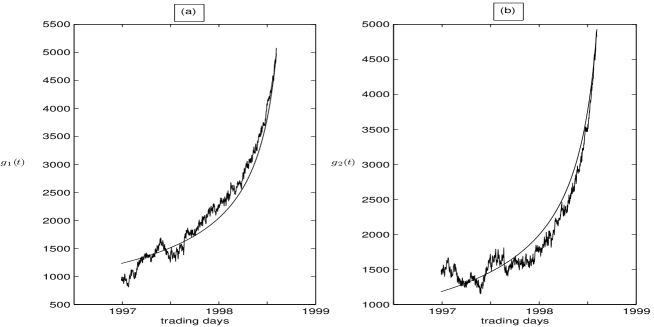
Figure 3: Sampling drawn accordingly to $g_{1}(t)$ (8) (fig. (a)) and $g_{2}(t)$ (9) (fig. (b)). The curves correspond to the critical level for $\bar{f}(t)$, i.e. $g^{+}$ (fig. a) and $g^{-}$ (fig. b). $g_{1}(t)$ and $g_{2}(t)$ replicate the deterministic exponential trend, the avalanche exponent $\tau$ and the $H$ self-similarity exponent of the NASDAQ index (see Fig. 2 for more details on $H$ statistics)

Table 1 resumes the values of NASDAQ avalanches under $g^{+}=\exp(F(t))+\theta+\gamma\bar{f}_{c}$, and of recoveries of $g_{2}(t)$ to $g^{-}=\exp(F(t))+\theta^{\prime}-\gamma^{\prime}\bar{f}_{c}$, that correspond to the critical level $\bar{f}_{c}$ for $\bar{f}(t)$. Figs. 3(a) and 3(b) show samplings of (8) and (9). Notice the mirror symmetry w.r.t. $g^{+}$ and $g^{-}$. We are going to use $g_{1}(t)$ in order to model avalanches, and $g_{2}(t)$ in order to model recoveries. We are going to use the above results in Sec. 4 in order to give an estimate of the probability of $g^{+}$ and $g^{-}$ crossing and trend line slope and location.

3 Technical analysis signals

Technical analysis [29] is based on the reaction of financial agents to market conditions as they can be detected through the study of charts, i.e. financial market data plot. It is characterized by the usage of particular signals in order to trigger buy/sell orders.

The most significant criticism against such a technique is its possible lack of precision in the recognition of signal patterns and its subjective judgement in their interpretation. These could mislead to the precise timing of signals. In spite of this uncertainty it is worth remarking that the methods have been surviving and developing for a long time. This consideration suggests to look for the extraction of the essence of the methods not affected by any psychological effect but which can be detected by an automatic decision support system properly calibrated.

TA signals are triggered by the occurrence of some patterns, that can be separated further on. The easiest figures to deal with and which can provide useful trading information are horizontal barriers. An immediate further step is given by the crossing of lines with a not null slope, like trend lines, fan lines, and channels. Trend lines are straight lines joining sequences of at least two minima (maxima) with the second one higher (lower) than the first one; fan lines are trend lines joining two points: the first one is kept fixed (it is common to all of them), and it is a minimum (maximum), while the second point is given by the subsequent minimum (maximum). Channels can be drawn in the case for which the data exhibits a sequence of minima with linearly growing height and a sequence of maxima with approximately the same linearly growing height. In this case the line fitting the sequence of maxima and the line fitting the sequence of minima identify a channel. The identification of the above quantities is highly sensitive to the time scale that is chosen, as moving averages and their relative crossing are [59].

Buy/sell signals rely on the identification of particular configurations. Several rules are known for their identification [23]. They provide a set of buy/sell triggering orders more complex than the simple crossing of an horizontal barrier. However the knowledge and the understanding of the base components are the starting points towards the analysis of more complex patterns.

Recently TA has been reconsidered and strategies redefined in order to take into account not only the price variation but also the effect of volume bearing upon classical mechanics ideas [60, 61]. Although the volumes play an important role in technical analysis their examination is also outside the scope of this paper.

4 Self-barrier crossing

As recalled here above, the probability of avalanche duration in Self-Organizing Critical systems can be used for modeling the probability of falls in markets, thus carrying on the comparison with the earthquake theory, as it has been evidenced across the literature on large financial crashes [28].

Here below, it is shown how to use the property of the model previously discussed in order to estimate the probability of the expected time for line crossings. For this crossing search we use the data self generated values. i.e. $g^{+}$ and $g^{-}$ defined in Sec. 2.4 so that we call the problem self-barrier crossing in analogy with self-avoiding walk wording [62].

4.1 Line crossing estimate based on the model structure

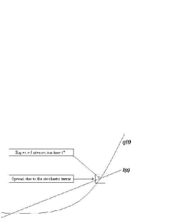
Figure 4: Line crossing

Let $l(t)=a\,t+b$ be a straight line, see Fig. 4. Let $g(t)$ be either $g_{1}(t)$ or $g_{2}(t)$. The average

$$q(t)=<g(t)>$$

is equal to

$$q(t)=\exp(F(t))+\theta+\gamma<\bar{f}(t)>$$

in the case $g(t)=g_{1}(t)$, and to

$$q(t)=\exp(F(t))+\theta^{\prime}+\gamma^{\prime}<-\bar{f}(t)>$$

in the case $g(t)=g_{2}(t)$. The function $q(t)$ is a deterministic function of $t$, and the expected intersection time $t=t^{*}$ for the line crossing can be calculated by

$$q(t*)=l(t*).$$ (11)

In the case $g(t)=g_{1}(t)$ the error on $t^{*}$ can be deduced from $\gamma Var(\bar{f}(t))$. This provides an estimate about the spread around the expected time for the process to cross any line (Fig. 4).

Since it is known that the maximal change in $s$ steps, $\forall t\in[1,T]$, is $\max\mid\bar{f}^{d}(t+s)-\bar{f}^{d}(t)\mid 5s/L^{d}$ [52] it is found that the $\max$ and $\min$ slope between two points $(t,g_{1}(t))$ and $(t+s,g_{1}(t+s))$ are given by

$$(e^{F(t+s)}-e^{F(t)}\pm\gamma\frac{5s}{L^{d}})\frac{1}{s}.$$ (12)

Analogous results hold for $g(t)=g_{2}(t)$. In order to tighten bounds on slopes let us analyze the distribution of the slopes of lines joining $(t,\exp(y(t)))$ and $(t+s,\exp(y(t+s)))$, $(t,g_{1}(t))$ and $(t+s,g_{1}(t+s))$, and $(t,g_{2}(t))$ and $(t+s,g_{2}(t+s))$, respectively, for $s=2,3,4,11,13$, that are values significant for the NASDAQ avalanches and recoveries.

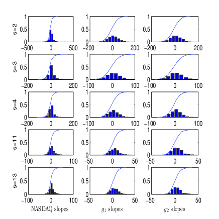
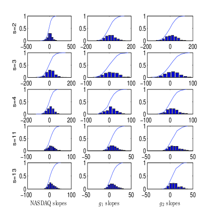
(a)                                                              (b)

Figure 5: Histograms and cumulative function of the distribution of the slopes of lines joining $(t,\exp(y(t)))$ and $(t+s,\exp(y(t+s)))$, $(t,g_{1}(t))$ and $(t+s,g_{1}(t+s))$, and $(t,g_{2}(t))$ and $(t+s,g_{2}(t+s))$, respectively, for $s=2,3,4,11,13$. (a) Analysis on the entire time series. (b) Analysis on the time series since December 23${}^{th},1998$

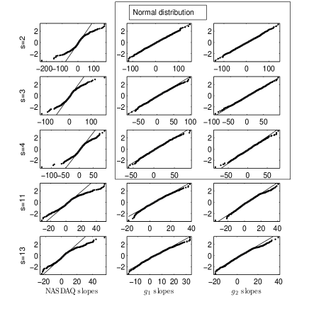
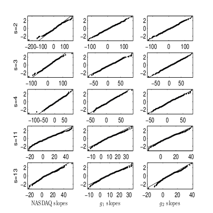
(a)                                                              (b)

Figure 6: Normal distribution hypothesis testing of data reported in Fig. 5. The solid line corresponds to the normal distributed value with the same mean and variance of raw data (represented by dots). (a) Analysis on the entire time series. Both the Lilliefors and the Jarque-Bera test reject the normal hypothesis distribution at $95\%$ confidence level in all the NASDAQ cases and for the biggest values of $s=11$ and $s=13$ also on $g_{1}$ and $g_{2}$ . (b) Analysis on the time series since December 23^th, 1998. The Lilliefors test rejects the normal hypothesis distribution at $95\%$ confidence level in the NASDAQ cases $s=2$, $s=13$, and on $g_{1}$ for $s=11$; the Jarque-Bera test provides the same results given on the entire series, apart on the NASDAQ case for $s=11$, in which it does not reject the normal hypothesis distribution

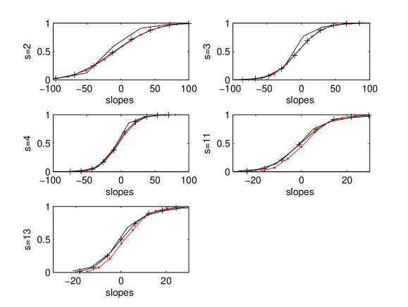
(b)

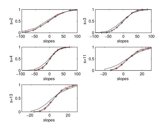
Figure 7: For each avalanche size $s$ the cumulative functions of the distribution of the slopes of lines joining $(t,\exp(y(t)))$ and $(t+s,\exp(y(t+s)))$ (solid line), $(t,g_{1}(t))$ and $(t+s,g_{1}(t+s))$ (line with crosses), and $(t,g_{2}(t))$ and $(t+s,g_{2}(t+s))$ (line with dots) are plotted together for comparison. The frequency of the slopes of $g_{1}$ and $g_{2}$ around the mean are lower bounds for the NASDAQ slopes. (a) Analysis on the entire time series. The deviation of the NASDAQ from the normal distribution and the leptokurtosis is evidenced at most for $s=2$. (b) The same analysis performed on the time series since December 23^th, 1998. Deviation of the NASDAQ from the normal distribution is best evidenced for $s=2$

The analysis is carried on both the entire NASDAQ time series (Figs. 5(a), 6(a), and 7(a)) and the best fitted subperiod starting on December 23^th, 1998 (Figs. 5(b), 6(b), and 7(b)). Due to the avalanche distribution the most frequent value is lower than the median, that is lower than the mean. Fig. 5 reports the histograms and their cumulative distribution. For each fixed time step $s$ the frequency of the slope of lines joining points with time distance $s$ (either on the raw data or on the simulated ones) can be obtained directly from the histogram. A trader would examine how many percentage of the slopes is between two bounds in order to estimate the risk of some strategy.

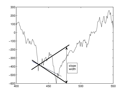
Figure 8: An example of 10% interval of slopes (upper and lower lines) together with a line actually joining $(t,g_{1}(t))$ and $(t+s,g_{1}(t+s))$ with $s=2$

As an example, referring to Fig. 5(a), the $75\%$ of the slopes are in a interval of width the standard deviation around at the mean, whilst $10\%$ are in a more tight interval with width $2.3$ (see Fig. 8).

On the entire time series both the Lilliefors and the Jarque-Bera test reject the normal hypothesis distribution at $95\%$ confidence level in all the NASDAQ cases and for the biggest values of $s=11$ and $s=13$ also on $g_{1}$ and $g_{2}$ (Fig. 6(a)). On the NASDAQ data set starting on December 23^th, 1998 both tests reject the normality hypothesis only for $s=2$ and $s=13$ (Fig. 6(b)). Table 2 resumes the values of mean and standard deviation on both the entire time series and on data since December 23^th, 1998. It is worth noting the relationship between the slopes distributions of the NASDAQ, $g_{1}$, and $g_{2}$ (Fig. 7). Their comparison shows the probability of the occurrence of slopes joining points at time step distance corresponding to the most frequent avalanche size, to the median, and to the mean. The NASDAQ distribution is higher around at its mean in all the reported samples. The frequency of the slopes of $g_{1}$ and $g_{2}$ around at the mean is a lower bound for the NASDAQ slopes. The evaluation of bounds relevant for particular strategies is left for future work.

In TA trend lines must be drawn by joining either decreasing sequences of maxima (at least two), or increasing sequences of minima [23]. No method seems available up to now in order to forecast whether the second maximum (minimum) is lower (higher) than the first one, thus giving rise to a trend line [23]. However because the deterministic part of $g(t)$ is strictly monotonous it is possible to calculate some bounds: the minimum time $s$ such that $g(t+s)>g(t)$, is given by $\exp(F(t+s))-\exp(F(t))>\gamma 5s/L^{d}$. The maximum time $s$ such that the inequality $g(t+s)<g(t)$ can hold is given by $\exp(F(t+s))-\exp(F(t))<\gamma 5s/L^{d}$.

4.2 Trend line detection

Trend lines [23] play an important role because they serve as a basis for classical technical analysis. Such lines are drawn joining a sequence of at least two maxima (minima) with the second one lower (higher) than the first one, each one being selected as global maxima (minima) on time windows [23]. The size of time windows depends on the information that the analyst is looking for. Thus to trace out trend lines strictly depends on the time width that is chosen. Major trends are defined by the Dow theory as trends during more than one year, although this limit can be lowered to six months on the future market. Thus in this case maxima (minima) can be looked for on monthly time windows. At the opposite time window size choice there are short time trends, that are shorter than two $-$ three weeks. Intermediate trends should take into account periods of two $-$ three weeks up to several months. They are more stable than those observed on short time intervals [23], and more meaningful than those over long time intervals, on which the exponential trend is already visible.

Any upward (downward) peak can be considered as a maximum (a minimum) and can be used for trend line identification. On the NASDAQ and on the BS simulations the peaks occur any $2-3$ steps, thus short time trend lines could be drawn and the results on the previous section could be directly applied.

However the choice of the time window where to look for global maxima much relies on the feeling of the analyst. We stress that the BS model can provide a further contribution about the occurrence of trend lines in the case in which the investor is not interested to peaks inside the avalanche, even if they are local maxima in their time window.

Information model$-$related furnishes estimates on the occurrence of two maxima separated by an avalanche. Their time steps distance is bigger than the time width of an avalanche. The function $g_{1}(t)$ takes into account avalanches following the definition of the Li-Cai model [51], and the function $g_{2}(t)$ considers recoveries.

Henceforth the function $g_{1}(t)$ can provide information about the time steps distance of values separated by an avalanche, thus about the minimal distance between maxima separated by an avalanche. On the other hand the function $g_{2}(t)$ can provide information about the time steps distance of values separated by a recovery, thus about the occurrence of minima. This kind of approach can be useful to set up automatic trading rules that trigger orders on the basis of the occurrence of falls in the market, or in the case of the end of a small bubble and of the return to the fundamental price.

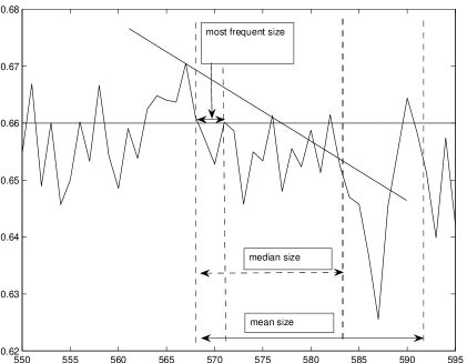
Figure 9: A sampling of $\bar{f}^{d}(t)$. The most frequent size of an avalanche is smaller than the median size, that is smaller than the mean

The BS model shows a distribution of avalanche sizes which decays as a power law with the size of the avalanches. Thus the most frequent value is much smaller than the mean (Fig. 2(c)). An investor can thus practically estimate the probability to have a short time avalanche instead of a medium size one directly from frequencies of avalanches sizes. Because of the asymmetry of the frequency distribution of an avalanche sizes, that is limited by 0 on its left, and that has power law tail on the right, the most frequent values are the smallest ones ($1$ and $2$ time steps below the threshold, i.e. avalanche sizes $2$ and $3$); notice that the median of the avalanche size is lower than the mean (Fig. 9).

The above remarks evidence once more that short time trend lines - even separated by an avalanche $\bar{f}^{d}(t)$- are the most frequent.

Thus downward trend lines can be considered for short time intervals, but not for medium size ones. Anyway in a growing market downwards trend lines are surely going to be crossed; the most interesting question is about the upward trend lines that join sequences of local minima which height is increasing.

The function $g_{2}(t)$ can be used in order to give estimates of distances between minima separated by recoveries. Its structure of recoveries is mirroring the structure of BS ordinary avalanches. Thus the mean distance between two minima separated by a recovery is bigger than the avalanche size. Here again the short time recoveries are the most frequent ones, but in this case the second minimum could not be higher than the first one. Due to the exponential term, the median and the mean size recoveries separate minima with the second one higher than the first one.

5 Conclusions

Any automatic trading system can trigger buy/sell orders when some either upper or lower barrier is crossed. Rules like these, even so simple, have been able to cause crashes in markets. Technical analysis studies concern a more complex structure of signals and often rely on the sensitivity of the analyst.

We have observed an analogy between statistical properties of a coevolution model, in particular the avalanche content description, with the residuals of a financial index signal like the NASDAQ 100 Composite - residuals obtained from the latter signal first order approximation obtained by the theory of large financial crashes.
In view of the analytical properties of the superposition of such a microscopic models, we have been able to derive estimates for avalanche and recovery duration time. We have pointed out the qualitative features helping technical analysts to elaborate more refined approached than classical ones. Several quantitative features are also available. Other indices could be used for a search on universality properties. We stress that we have discussed not only degradation, but also recovery features.

The suitability of the mean fitness properties for bubble models as they emerge from the BS model dynamics does not stop at the level of numerical analysis of correlations, but goes further into the dependence structure of avalanches, making this approach a sound complement to the fBm approach. Moreover the BS model furnishes an agent-based model for an explanation of the cooperative behavior that leads to the earthquake and large financial crashes phenomena, thus embracing simulations into a theoretical framework that allows to state the reliability of the results apart from numerical instabilities.

The set up of a model for the residuals provides a further insight on the formation of trend lines. Statistics drawn on the BS model about the occurrence of trend lines slopes provide market analyst by bounds of the probability of the occurrence of trend lines on market index data. Moreover, once trend lines are drawn, the probability of their crossing can be estimated from the model. This is a first step towards other signal technical analysis and to the assessment of the usage of technical analysis rules that supersede the skill of the single analyst.

In addition the 2-dimensional model, necessarily implying the existence of more than 2 nearest neighbor agents, obviously 4 for the square lattice data examined here above, finds some correspondence in the sand pile model on a fractal basis simulating financial avalanches before a crash as studied in references [24, 39] where the periodicity of the log periodic oscillations indicate that the relevant number of agents is between 3 and 4.

For further work, it could be suggested that more complex signals be examined, together with a deeper analysis of the fractal and multifractal structure both of the microscopic model and of market data.

Acknowlegements

MA thanks EC Project ’Extreme events: Causes and consequences (E2-C2)’, Contract No 12975 (NEST) for some financial support.

6 Appendix

In this appendix we outline a few results corresponding to those on the main text, but in which a $1$-dimensional model rather than a $2$-dimensional model is used. We recall that $\bar{f}^{1}_{c}=0.8335$; the value of $\tau$ for avalanches in the Li-Cai spirit is $\tau=1.80$ [52] and it is the same degradations or recoveries.

The estimate of $H$ fluctuates around at 0.07. These values are rather far from the NASDAQ data indicating poor agreement with a $1$-dimensional model.

The long term memory property of a time series can be estimated through its components: it is reported in [11] that the sum of two independent fractionally integrated processes of order, respectively, $d$ and $d^{\prime}$ is $\max\{d,d^{\prime}\}$. The relationship $H=d+1/2$ [63] allows to deal with a fBm $z_{H}(t)$, $H=d+1/2$ in order to fix $\theta$, $\gamma$, $\zeta$, $H$ such that

$$\theta+\gamma\bar{f}(t)+\zeta z_{H}(t)$$ (13)

has the same self similarity exponent and the same range of $R(t)$.

Whilst the contribution of $\bar{f}(t)$ is due to the local agent interactions, the contribution of $z_{H}(t)$ can be interpreted either like the contribution of noise traders, in the case of uncorrelated signal, or like the presence of fundamentalist traders in the market whether a mean reverting process occurs [22]. This gives an interesting perspective about the level of SOC that can be masked by either noise or fundamentalists traders. However for the purposals of this paper to give an evaluation tool for the crossing of lines this model would give more weak results. As an example in (11) the variance about the expected crossing time would contain also the variance term due to the presence of fBm. Also the BS structure of avalanches would be modified, moreover a model of data based uniquely on fBm would result more simple, and so preferable to (13). Thus the choice of the $2$-dimensional BS models meets the task to give simple description at a microeconomic level more meaningful of those related to a generic fBm, with the maintainance of properties (self-similarity, avalanches and recoveries) at the macro level more suitable for data than the $1$-dimensional BS model.

Table 1: Avalanche and recovery size estimates. According to definition the minimum sized avalanche stays only one time step below the threshold, giving rise to avalanche size $s=2$

NASDAQ	$\tau$	avalanche size
		most frequent	median	mean
avalanche below $g^{+}$	0.72 ( 0.18,1.25)	3(28$\%$)	4	13
recoveries to $g^{-}$	$1.79(1.33,2.25)$	2(38$\%$)	4	11

Table 2: Mean and standard deviation (between the parentheses) of the slopes of lines joining $(t,\exp(y(t)))$ and $(t+s,\exp(y(t+s)))$ (NASDAQ), $(t,g_{1}(t))$ and $(t+s,g_{1}(t+s))$ ($g_{1}$), and $(t,g_{2}(t))$ and $(t+s,g_{2}(t+s))$ ($g_{2}$) for $s=2,3,4,11,13$: (a) Analysis on the entire time series; (b) Analysis on the time series since December 23^th, 1998

(a) data $s=2$ $s=3$ $s=4$ $s=11$ $s=13$ NASDAQ $4.51(39.1561)$ $4.52(27.3603)$ $4.45(22.3469)$ $4.24(12.0141)$ $4.18(10.8556)$ $g_{1}$ $4.95(44.2339)$ $4.90(29.1199)$ $4.86(22.3350)$ $4.72(9.5639)$ $4.69(8.6526)$ $g_{2}$ $4.04(44.3814)$ $4.05(29.4014)$ $4.06(22.8014)$ $3.92(10.6265)$ $3.87(9.7463)$

(b) data $s=2$ $s=3$ $s=4$ $s=11$ $s=13$ NASDAQ $9.36(55.5312)$ $9.29(38.3107)$ $9.05(30.9240)$ $8.42(15.6117)$ $8.27(13.8854)$ $g_{1}$ $8.98(46.0860)$ $8.89(30.1768)$ $8.71(23.2664)$ $8.31(9.7973)$ $8.23(8.8547)$ $g_{2}$ $9.53(46.1976)$ $9.50(30.4889)$ $9.57(23.8624)$ $9.21(11.2231)$ $9.09(10.2732)$

(a)

References

- [1] T. Bollerslev, H.O. Mikkelsen, J. Econometrics 73 (1996) 151-184.
- [2] F.J. Breidt, N. Crato, P. De Lima, J. Econometrics 83 (1998) 325-348.
- [3] R. Cont, J. da Fonseca, in Takayasu, H (Ed.), Empirical science of financial fluctuation, pp. 230-239, Springer , Tokyo, 2002.
- [4] A.W. Lo, Econometrica 59 (1991) 1279-1313.
- [5] Z. Ding, R.F. Engle, C.W.J. Granger, J. Empir. Fin. 1 (1993) 83- 106.
- [6] Z. Ding, C.W.J. Granger, J. Econometrics, 73 (1996) 61-77.
- [7] Z. Ding, C.W.J.Granger, J. Econometrics, 73 (1996) 185-215.
- [8] D. Sornette, A. Helmstetter, Phys. Rev. Lett. 89 (2002) 158501 -158504.
- [9] M. Ausloos, N. Vandervalle, in Fractals and beyond. Complexity in the Sciences, M.M. Novak, Ed., World Scientific, Singapore, (1998) 355-356.
- [10] B.B. Mandelbrot, J.W. Van Ness, SIAM Review 10 (1968) 422-437.
- [11] C.W.J. Granger, J. Econometrics 14 (1980) 227-238.
- [12] C.W.J. Granger, R. Yoyeux, J. Time Series Anal. 1 (1980) 15-29.
- [13] A. Krawiecki , J.A. Holyst, Physica A 317 (2003) 597 - 608.
- [14] M. Lippi, P. Zaffaroni, Contemporaneous Aggregation of Linear Dynamic Models in Large Economies, Manuscript, Research Department, Bank of Italy (1999).
- [15] P. Zaffaroni, Contemporaneous aggregation of GARCH processes, preprint, (1999).
- [16] P. Zaffaroni, Aggregation and memory of models of changing volatility, preprint, (2001).
- [17] D. Blake, in ”Financial market Analysis, 2nd Ed.” (Wiley, Chichester, 2000) p.455.
- [18] R. Cerqueti, G., Rotundo, G., Proceedings of IEEE International Conference on Computational Intelligence for Financial Engineering (CIFEr2003), 20-23 March 2003, Hong Kong.
- [19] A. Kirman, in ”Money and Financial Markets”, chap. 17, M. Taylor Ed., Macmillan London, 1991.
- [20] A. Kirman, Quaterly J. Economics 108 (1993) 137-156.
- [21] A.P. Kirman, G. Teyssiére G., Microeconomic Models for Long-Memory in the Volatility of Financial Time Series, preprint GREQAM DT 00A3 (2000).
- [22] J.-P. Fouque, G. Papanicolaou, K.R. Sircar, Mean-Reverting Stochastic Volatility. Preprint, November 1998.; see also .
- [23] J.J. Murphy, Technical analysis of the Futures Markets, Prentice Hall, New York, 1986.
- [24] M. Ausloos, K. Ivanova, N. Vandervalle, in ”Empirical sciences of financial fluctuations. The advent of econophysics”, H. Takayasu, Ed. (Springer Verlag, Berlin, 2002) pp. 62-76.
- [25] A. Johansen, O. Ledoit, D. Sornette, Int. J. Theo. Appl. Finance (3) (2000) 219-255.
- [26] A. Johansen, D. Sornette, Euro. Phys. J. B 17 (2000) 319-328.
- [27] N. Vandervalle, M. Ausloos, Ph. Boveroux, A. Minguet, , Eur. Phys. J. B 4 (1998)139-141.
- [28] N. Vandervalle, Ph. Boveroux, A. Minguet, M. Ausloos, Physica A 255 (1998) 201-210.
- [29] J.V. Andersen, S. Gluzman, D. Sornette, Eur. J. Phys. B 14 (2000) 579-601.
- [30] P. Bak, K. Sneppen, Phys. Rev. Lett. 71 (1993) 4083-4086.
- [31] A. Johansen, D. Sornette , Endogenous versus Exogenous Crashes in Financial Markets, Contemporary Issues in International Finance, (2004). In press.
- [32] A. Johansen, D. Sornette, Int. J. Theo. Appl. Finance 4 (2001) 853-920.
- [33] W.X. Zhou, D. Sornette, Physica A 329 (2003) 249-263.
- [34] E. F. Fama, J Business 8 (1965) 1.
- [35] G. Rotundo, in ”The Logistic Map and the Route to Chaos: From the Beginning to Modern Applications” Ausloos M. and Dirickx M. eds. (Springer, Berlin, 2006) pp. 239-258.
- [36] S. Drozdz, F. Ruf, J. Speth, M. Wojcik, Eur. Phys. J. B 10 (1999) 589-593.
- [37] J.A. Feigenbaum, P.G.O. Freund, Int. J. Mod. Phys. B 10 (1996) 3737-3745.
- [38] T. Kaizoji, Physica A 287 (2000) 493-506.
- [39] N. Vandervalle, R. D’hulst, and M. Ausloos, Phys. Rev. E 59 (1999) 631-635.
- [40] M. Ausloos, in From Quanta to Societies, W. Klonowski, Ed. (Pabst, Lengerich, 2002) pp. 88-106.
- [41] Z. Chen, P. Ch.Ivanov, K. Hu, H.E. Stanley, Phys. Rev. E, 65 (2002) 041107(15).
- [42] K. Hu, P.Ch. Ivanov, Z. Chen, P. Carpena, H.E. Stanley, Phys. Rev. E 64 (2001) 011114.
- [43] M. Ding, W. Yang, Phys. Rev. E 52 (1995) 207-213.
- [44] G. Rangarajan, M. Ding, Phys. Lett. A 273 (2000) 322-330.
- [45] T. S. Ray, N. Jan, Phys. Rev. Lett. 72, 4045 (1994).
- [46] K. Sneppen, Physica A 221 (1995) 168-179.
- [47] F. Guzzetti, B.D. Malamud, D.L. Turcotte, P. Reichenbach, Earth Planetary Sci. Lett. 195 (2002) 169-183.
- [48] K. Ito, Phys. Rev. E 52 (1995) 3232-3233.
- [49] F. Lillo, R.N. Mantegna, Power law relaxation in a complex system: Omori law after a financial market crash, preprint.
- [50] A. Krause, in: Namatame, A., Green, D., Aruka, Y. and Sato, H. (eds.): ”Complex Systems 2002: Complexity with Agent-based Modeling, Proceedings of the 6th International Conference on Complex Systems”, Chuo University, Tokyo 2002, pp. 278-283.
- [51] W. Li, X. Cai, Phys. Rev. E 61 (2000) 771-775.
- [52] W. Li, X. Cai, Phys. Rev. E, 61 (2000) 5630-5633.
- [53] W. Li, X. Cai, Phys. Rev. E 62 (2000) 7743.
- [54] M. Ausloos, P. Clippe, and A. Pekalski, Physica A 332 (2004) 394-402.
- [55] M. Paczuski, S. Maslov, P. Bak, Phys. Rev. E 53 (1996) 414.
- [56] T. Yamano, Int. J. Mod. Phys. C (in press).
- [57] C. Lee, X. Zhu, Gao Kelin, Nonlinearity 16 ( 2003) 25-33.
- [58] D. Sornette, A. Johansen, J.P. Bouchaud, J.Phys.I France 6 (1996) 167-175.
- [59] N. Vandervalle, M. Ausloos, Ph. Boveroux, Physica A 269 (1999) 170-176.
- [60] M. Ausloos, K. Ivanova, Eur. Phys. J. B 27 (2002) 177 -187.
- [61] M. Ausloos, K. Ivanova, in The applications of econophysics, H. Takayasu, Ed. (Springer Verlag, Berlin, 2004) pp. 117-124.
- [62] J. Rudnick, G. Gaspari, Elements of the Random Walk, Cambridge Univ. Press, Cambridge, 2004.
- [63] P. Embrechts, M. Maejima, Selfsimilar Processes Princeton Series in Applied Mathematics, ISBN 0-691-09627-9.