Impact of Boundary Conditions on Entrainment and Transport in Gravity Currents

Abstract

Gravity currents have been studied numerically and experimentally both in the laboratory and in the ocean. The question of appropriate boundary conditions is still challenging for most complex flows. Gravity currents make no exception - appropriate, physically and mathematically sound boundary conditions are yet to be found. This task is further complicated by the technical limitations imposed by the current oceanographic techniques.

In this paper, we make a first step toward a better understanding of the impact of boundary conditions on gravity currents. Specifically, we use direct numerical simulations to investigate the effect that the popular Neumann, and less popular Dirichlet boundary conditions on the bottom continental shelf have on the entrainment and transport of gravity currents.

The finding is that gravity currents under these two different boundary conditions differ most in the way they transport heat from the top towards the bottom. This major difference occurs at medium temperature ranges. Entrainment and transport at high temperatures also show significant differences.

Key words: Gravity Currents, Entrainment, Transport, Boundary Conditions, Boussinesq Approximation, Energy Equation

1. Applied Mathematics Department, Illinois Institute of Technology, Chicago, Illinois

2. Argonne National Laboratory, Darien, Illinois

3. RSMAS/MPO,University of Miami, Miami, Florida

4. Department of Mathematics, Virginia Polytechnic Institute and State University, Virginia

1 Introduction

A gravity or density current is the flow of one fluid within another caused by the temperature (density) difference between the fluids [1]. Gravity currents flowing down a sloping bottom that occur in the oceans (e.g., those that flow down the Strait of Gibraltar and the Denmark Strait) are an important component of the thermohaline circulation [2], which in turn is important in climate and weather studies.

Oceanic gravity currents have been studied in the past, both in the laboratory and in the ocean. They have been modelled in various ways, starting from the streamtube models, e.g., [3, 4] to more recent non-hydrostatic Boussinesq equations [5, 6, 7].

The question of appropriate boundary conditions for complex flows, such as the gravity currents we consider in this paper, is still challenging. This paper is a first step in an effort to bridge the gap between observed gravity currents and the assumptions made in modeling them. Using ocean observations to develop realistic boundary conditions for gravity currents is limited by the available technological means. Thus, the current boundary conditions used in the numerical simulation of gravity currents are based on physical intuition and mathematical simplicity and soundness.

The behavior of gravity currents under two different types of boundary conditions is studied in this paper. Specifically, the differences between gravity currents flowing with Neumann (insulation) and Dirichlet (fixed-temperature) bottom boundary conditions are investigated via direct numerical simulations. Quite possibly, other boundary conditions, such as Robin, would be more appropriate. However, given the popularity of Neumann [5, 8, 9, 10, 29] and, to a lesser extent, Dirichlet boundary conditions in numerical studies [11], we decided to focus first on these two types of boundary conditions.

Bottom Neumann boundary conditions for temperature may be assumed when the material on the continental shelf is a bad thermal-conductor (i.e., the current flows over “insulated” rock). Dirichlet boundary conditions may be assumed when the material on the continental shelf is a good thermal-conductor, making temperature nearly constant [12].

Dirichlet boundary conditions would be appropriate for the initial transient development of gravity currents. For instance, it is known that the Red Sea overflow shuts off in the summer [13]. Once this gravity current starts again, one could expect the temperature difference between the bottom layer and the overflow to have a transient impact on the mixing near the bottom. Also, such a temperature gradient could significantly affect the initial neutral buoyancy level, which is of ultimate interest for large-scale ocean and climate studies. Özgökmen et al. [14] found in numerical simulations that the neutral buoyancy level did not differ significantly from an analytical estimate, which does not account for mixing, because the bottom layer properties were isolated from vigorous mixing between the gravity current and the ambient fluid, and yet determined the neutral buoyancy level. Thus, any mechanism that can affect the properties of near bottom fluid is likely to change the neutral buoyancy level, at least during the initial stages of the development. This idea will be explored in a future study.

The rest of the paper is organized as follows: Section 2 presents the mathematical model used in our numerical study. Section 3 presents the numerical model used and the model configuration and parameters. Section 4 presents the velocity and temperature boundary and initial conditions used in the numerical simulation. Section 5 presents the numerical investigation of the effect of Neumann and Dirichlet boundary conditions on the bottom continental shelf on entrainment and transport in gravity currents. Five different metrics are used to this end. Finally, Section 6 presents a summary of our findings and directions of future research.

2 Mathematical Setting

Consider a two-dimensional gravity current flowing downstream, with x as the horizontal (downstream) direction, and z the vertical direction (Fig. 1).

The momentum and continuity equations subject to the Boussinesq approximation can be written as:

$$\frac{\partial u}{\partial t}+u\frac{\partial u}{\partial x}+w\frac{\partial u}{\partial z}=-\frac{1}{\rho_{0}}\frac{\partial p}{\partial x}+\nu_{h}\frac{\partial^{2}u}{\partial x^{2}}+\nu_{v}\frac{\partial^{2}u}{\partial z^{2}}\;,$$ (1)

$$\frac{\partial w}{\partial t}+u\frac{\partial w}{\partial x}+w\frac{\partial w}{\partial z}=-\frac{1}{\rho_{0}}\frac{\partial p}{\partial z}-g\frac{\rho^{\prime}}{\rho_{0}}+\nu_{h}\frac{\partial^{2}w}{\partial x^{2}}+\nu_{v}\frac{\partial^{2}w}{\partial z^{2}}\;,$$ (2)

$$\frac{\partial u}{\partial x}+\frac{\partial w}{\partial z}=0\;,$$ (3)

where $(x,z)$ are the two spatial dimensions, $t$ the time, $(u,w)$ the two velocity components, $p$ the pressure, $g=9.81\,m^{2}s^{-1}$ the gravitational acceleration, and $\nu_{h}$ and $\nu_{v}$ the viscosities in the horizontal and vertical directions, here assumed to be constants. The way these viscosities appear in the simulations is actually via their ratio, $r=\nu_{v}/\nu_{h}$.

One can argue that, at the horizontal scale being studied ($10$ km), we may assume a constant horizontal viscosity, $\nu_{h}$, since its controlling factors, model resolution and the speed of the gravity current (the fastest signal in the system), do not warrant a variable horizontal viscosity.

At the scale at which these experiments were conducted, which is similar to that in Özgökmen and Chassignet [9], rotation is not considered important either, i.e., vertical rigidity is not assumed [15]. In addition, it is also known that the vertical diffusion in the ocean is small [16]. It is precisely the theory that vertical mixing between gravity currents and the ambient fluid is via eddy-induced mixing and entrainment, not by diffusion, that led to the assumption that the vertical viscosity may likewise be taken to be constant, and assumed to be small, in fact. The ratio $r=\nu_{v}/\nu_{h}$ is kept at $r=0.5*10^{-3}$, under the range that Özgökmen and Chassignet estimate the results to be insensitive to the values of the vertical viscosity.

A linear equation of state is used

$$\rho^{\prime}=-\rho_{0}\,\alpha\,T\;,$$ (4)

where $\rho_{0}$ is the background water density, $\alpha$ the heat contraction coefficient, and $T$ the temperature deviation from a background value. The equation for heat transport is

$$\frac{\partial T}{\partial t}+u\frac{\partial T}{\partial x}+w\frac{\partial T}{\partial z}=\kappa_{h}\frac{\partial^{2}T}{\partial x^{2}}+\kappa_{v}\frac{\partial^{2}T}{\partial z^{2}},$$ (5)

where $\kappa_{h}$ and $\kappa_{v}$ are thermal diffusivities in the horizontal and vertical directions, respectively. Nondimensionalizing by $(x,z)=H\,(x^{*},z^{*}),\;$ $(u,w)=\frac{\nu_{h}}{H},\;(u^{*},w^{*}),\;t=\frac{H^{2}}{\nu_{h}}\,t^{*},\;p=\frac{\rho_{0}\,\nu_{h}^{2}}{H^{2}}\,p^{*},\;$ $T=\Delta T\,T^{*},\;$ where $H$ is the domain depth and $\Delta T$ is the amplitude of the temperature range in the system, and dropping $(*)$, the equations become

$$\frac{\partial u}{\partial t}+u\frac{\partial u}{\partial x}+w\frac{\partial u}{\partial z}=-\frac{\partial p}{\partial x}+\frac{\partial^{2}u}{\partial x^{2}}+r\frac{\partial^{2}u}{\partial z^{2}}\;,$$ (6)

$$\frac{\partial w}{\partial t}+u\frac{\partial w}{\partial x}+w\frac{\partial w}{\partial z}=-\frac{\partial p}{\partial z}+Ra\,T+\frac{\partial^{2}w}{\partial x^{2}}+r\,\frac{\partial^{2}w}{\partial z^{2}}\;,$$ (7)

$$\frac{\partial u}{\partial x}+\frac{\partial w}{\partial z}=0\;,$$ (8)

$$\frac{\partial T}{\partial t}+u\frac{\partial T}{\partial x}+w\frac{\partial T}{\partial z}=Pr^{-1}\left(\frac{\partial^{2}T}{\partial x^{2}}+r\,\frac{\partial^{2}T}{\partial z^{2}}\right)\;,$$ (9)

where $Ra=(g\,\alpha\,\Delta T\,H^{3})/\nu_{h}^{2}$ is the Rayleigh number (the ratio of the strengths of buoyancy and viscous forces), $Pr=\nu_{h}/\kappa_{h}$ the Prandtl number (the ratio of viscosity and thermal diffusivity), and $r=\nu_{v}/\nu_{h}=\kappa_{v}/\kappa_{h}$ the ratio of vertical and horizontal diffusivities and viscosities.

We consider $0<r\leq 1$. This implies that the viscosity and diffusivity in either direction are proportional, and both are small. This is in line with the theory that diffusion plays only a small role in the vertical mixing between gravity currents and the ambient fluid, and the mechanism is via eddy-induced mixing and entrainment.

3 Numerical setting

3.1 Numerical model

The first consideration taken in passing from the mathematical to the numerical model was the small amount of physical dissipation. This calls for an accurate representation of the convective operator so that the numerical dissipation and dispersion do not overwhelm the assumed physical effects.

Secondly, since small-scale structures are transported with minimal physical dissipation, accurate long-time integration is required. Thus, high-order methods in space and time are needed. The presence of small-scale structures also implies a need for significant spatial resolution in supercritical regions, which may be localized in space.

The numerical method implemented by Nek5000, the software used in the simulations, is described below:

The spatial discretization of (6)–(9) is based on the spectral element method [17], a high-order weighted residual method based on compatible velocity and pressure spaces that are free of spurious modes Locally, the spectral element mesh is structured, with the solution, data and geometry expressed as sums of Nth-order Lagrange polynomials on tensor-products of Gauss or Gauss-Lobato quadrature points. Globally, the mesh is an unstructured array of K deformed hexahedral elements and can include geometrically nonconforming elements. Since the solutions being sought are assumed to be smooth, this method is expected to give exponential convergence with N, although it has only $C^{0}$ continuity. The convection operator exhibits minimal numerical dissipation and dispersion, which is required in this study. The spectral element method has been enhanced through the development of a high-order filter that stabilizes the method for convection dominated flows but retains spectral accuracy [18].

The time advancement is based on second-order semi-implicit operator splitting methods [19, 20]. The convective term is expressed as a material derivative, and the resultant form is discretized via a stable backward-difference formula.

Nek5000 uses an additive overlapping Schwarz method as a preconditioner, as developed in the spectral element context by Fischer et al. [21, 22]. This implementation features fast local solvers that exploit the tensor-product form, and a parallel coarse-grid solver that scales to 1000s of processors [23, 24].

3.2 Model configuration and parameters

The model domain (see Fig. 1) is configured with a horizontal length of $L_{x}=10\,km$. The depth of the water column ranges from $400\,m$ at $x=0$ to $H=1000\,m$ at $x=10\,km$ over a constant slope. Hence the slope angle is $\theta=3.5^{\circ}$, which is within the general range of oceanic overflows, such as the Red Sea overflow entering the Tadjura Rift [5].

Numerical simulations were successfully carried out at a Prandtl number $Pr=7$ and a Rayleigh number $Ra=320\times 10^{6}$.

The numerical experiments were conducted on a Beowulf Linux cluster consisting of 9 nodes with 1 Gbps ethernet connectivity. Each node has dual Athlon 2 GHz processors with 1024 MB of memory. The 2D simulations take approximately 72 hours (simulated to real time ratio of $\sim$ 3).

4 Velocity and temperature boundary and initial conditions

4.1 Temperature boundary conditions

Inlet

($x=0;\ 0.6\leq z\leq 1.0$): The temperature gradient is one of two agents driving the flow, the other being the velocity boundary conditions (see Section 4.2).

The Dirichlet (fixed-temperature) boundary condition is assumed at the inlet. This assumption is simple to work with, although its correctness ultimately depends on whether or not sea water is an excellent thermal conductor [12]. The boundary condition

$$T=\frac{1}{2}\left[1-\cos\left(\pi\frac{1-z}{0.4}\right)\right]\;,$$

and the initial condition

$$T=\frac{1}{2}\exp(-x^{20})\left[1-\cos\left(\pi\frac{1-z}{0.4}\right)\right]\;,$$

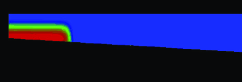
Figure 2: Color-coded density plot for temperature at time t=0; red is coldest, blue is least cold

are used (see Fig. 2). Figure 2 shows the initial color-coded density plot for temperature (red is lowest temperature, blue is highest).

Bottom

(the continental shelf): This is the interface between the gravity current and the continental shelf. The actual thermal conductivity of the continental shelf will suggest the proper boundary condition. Ockendon et al. [12] prescribe Dirichlet conditions if the boundary (the continental shelf) is an excellent thermal conductor; Neumann if the region outside of the gravity current (the continental shelf) is a very bad thermal conductor; and Robin when the thermal flux at the boundary is proportional to the difference between the boundary temperature and some ambient temperature. This last possibility was not studied in this paper, but could be the topic of further study, in the light of the results on incremental transport discussed later in this paper.

Surveys of the literature have not clarified the thermal conductivity of the continental shelf. The continental shelf is in the neritic zone, so it would contain a mixture of mineral and organic materials. In numerical simulations of gravity currents, the most popular choice is Neumann boundary conditions [5, 8, 9, 10, 29]. Fewer numerical studies employ Dirichlet boundary conditions [11]. Other boundary conditions (such as Robin) might be more appropriate and should be investigated. In this study, we focus on two different sets of boundary conditions: Neumann ($\partial T/\partial n=0$), and Dirichlet ($T=1$).

Dirichlet boundary conditions would be appropriate for the initial transient development of gravity currents. For instance, it is known that the Red Sea overflow shuts off in the summer [13]. Once this gravity current is initiated again, one could expect the temperature difference between the bottom layer and the overflow to have a transient impact on the mixing near the bottom. Also, such a temperature gradient could significantly affect the initial neutral buoyancy level, which is of ultimate interest for large-scale ocean and climate studies. Özgökmen et al. [14] found in numerical simulations that the neutral buoyancy level did not differ significantly from an analytical estimate, which does not account for mixing, because the bottom layer properties were isolated from vigorous mixing between the gravity current and the ambient fluid, and yet determined the neutral buoyancy level. Thus, any mechanism that can affect the properties of near bottom fluid is likely to change the neutral buoyancy level, at least during the initial stages of the development. This idea will be explored in a future study.

For Dirichlet boundary conditions, a nondimensional temperature of one was assumed.

Numerical experiments were conducted with shelf fixed-temperature values $0\leq T\leq 1$. $T=0$ had the effect of greatly speeding-up the gravity current, and not allowing the head to form. Thus, the current could not entrain ambient water at higher temperature values, contrary to experimental and oceanic observations.

Outlet

($x=10;\ 0\leq z\leq 1$): Note that the outlet is actually a sea water to sea water interface, since the region of interest (10 km) is only a small portion of the ocean’s breadth. The assumed boundary condition here is insulation, i.e. $\partial T/\partial\mathbf{n}=0$. (Another possible choice is the “do-nothing” boundary conditions [25].) Since the outlet is far away from the current for most of its journey down the continental shelf, the choice of boundary conditions will not influence significantly our numerical results.

Top

($z=1$): This is an air-sea water interface. Presently, insulation ($\partial T/\partial\mathbf{n}=0$) is assumed. Since air is a bad thermal conductor, this assumption is justified [12].

4.2 Velocity boundary conditions

Inlet

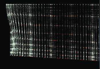
Figure 3: Velocity field at the inlet

($x=0;\ 0.6\leq z\leq 1.0$): Dirichlet velocity boundary conditions are used at the inlet. The velocity profile is given by an “S-shaped” polynomial function. The inlet velocity profile is one of the two forces that drive the flow, the other being the temperature gradient (see Section 4.1 and Figure 3).

Bottom

(the continental shelf): No-slip velocity boundary conditions ($u=0,w=0$) were used on the bottom. Previous studies on gravity currents by Özgökmen et al. [9, 5] assume no-slip velocity boundary conditions on the continental shelf, which is one of the most popular assumptions for fluids flowing over a solid boundary. Even in their studies on gravity currents over complex topography [10], which might constitute “roughness” and affect the log layer, Özgökmen et al. still used the no-slip assumption. One should note, however, that the question of appropriate boundary conditions flor fluid flows is still an active area of research. Other (more appropriate) choices include slip-with-friction boundary conditions [26, 27, 28]. Given the popularity of Dirichlet boundary conditions in numerical studies of fluid flows, however, we decided to focus on them first.

Interestingly, Härtel et al. [29] performed experiments on gravity currents at high Reynolds numbers for both slip and no-slip, and did not observe qualitative changes in the flow structure, although they did observe quantitative Reynolds number effects.

Outlet

($x=10;\ 0\leq z\leq 1$): Free-slip velocity boundary conditions ($\partial w/\partial x=0$, $\partial w/\partial y=0$, $\partial u/\partial x=0$, $\partial u/\partial y=0$) were used at the outlet. Another (more appropriate) choice is the “do-nothing” boundary conditions [25]. Since the outlet is far away from the current for most of its journey down the continental shelf, the choice of velocity boundary conditions will not influence significantly our numerical results.

Top

($z=1$): Free-slip velocity boundary conditions were used, similar to those used at the outlet.

Note that there are no boundary conditions imposed on pressure. To handle this, Nek5000 uses an operator splitting method, which initially uses a “guess for pressure”, corrects this guess (but velocity is now non-solenoidal), then corrects the velocity field to impose the divergence-free velocity field. See Rempfer [30] for a discussion of boundary conditions for pressure.

4.3 Velocity and temperature initial conditions

The initial velocity field is plotted in Fig. 3. The model is entirely driven by the velocity and temperature (Fig. 2) forcing functions at the inlet boundary ($x=0$), and the temperature gradient. The velocity distribution at this boundary matches no-slip at the bottom and free-slip at the top using fourth-order polynomials such that the depth integrated mass flux across this boundary is zero.

Other polynomials profiles may be assumed, but care must by taken to ensure that

• the depth-integrated mass flux across the boundary be zero;

• the assumed temperature profile be consistent with the flow reversal for the velocity boundary condition; and

• the amplitude of inflow velocity be time-dependent, and scaled with the propagation of the gravity current, otherwise there will be a recirculation at the inlet (in the case of over-estimation) or a thinning-down of the gravity current as it flows down-slope, in the case of under-estimation.

These considerations on initial conditions were taken into account by Özgökmen et al. [9, 10].

5 Numerical results

Gravity currents evolving with two different sets of boundary conditions (Neumann/insulation and Dirichlet/fixed temperature), are studied. Measurements were made of their entrainment, average temperature, and the heat each transports from the top (warmer water) towards the bottom (colder water).

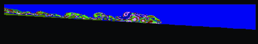
Figure 4: Gravity current with Neumann boundary conditions at time 6375 seconds

Figure 4 shows the gravity current with Neumann boundary conditions at 6375 seconds (real time). The head and secondary features are very visible at this point. One can see the current entraining some of the surrounding fluid via the Kelvin-Helmholtz instability, which is the main mechanism for mixing in a non-rotating fluid [9].

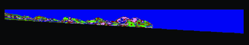
Figure 5: Gravity current with Dirichlet boundary conditions at time 6375 seconds

Figure 5 shows the gravity current with Dirichlet conditions, also at 6375 seconds. One can see a difference in the temperature distributions of the two currents, and it is such differences that this study tries to quantify.

The differences between the two currents are most notably in the way they transport heat, and in the way they entrain ambient water. In order to quantify the differences, five different metrics are used in Sections 5.1-5.5. These metrics allow a careful assessment of the effect of Dirichlet and Neumann boundary conditions on the numerical simulation of gravity currents.

5.1 Entrainment $E(t)$

This metric was earlier defined by Morton et al. [31]. The equivalent formulation of Özgökmen et al. [5] is used here:

$$E(t)=\frac{\mbox{$h-h_{o}$}}{\mbox{length}},$$ (10)

where $h$ is the mean thickness of the current from a fixed reference point (which is set at 1.28 km), and $h_{o}$ is the mean thickness of the tail. The length of the current is taken from the fixed reference point to the leading edge of the current. This metric gives us a sense of how ambient water is entrained into the gravity current.

The tail thickness, $h_{o}$, is calculated from the flux volumes passing through the fixed reference point. The mean thickness, $h$, is calculated from the total volume of the current, from the fixed reference point to the nose. The difference in volumes would be accounted for by the ambient water entrained.

The finding here is that the Dirichlet (fixed-temperature) boundary condition causes greater entrainment than Neumann (insulated) boundary condition, by about $14.21\%$, averaged over the entire travel time down the slope. This is actually consistent with the weighted temperature metrics (below), which say that the Neumann boundary conditions yield a colder current.

The maximum difference in $E(t)$ between the two currents occurs after the head has began to break-down, at around 10,000 seconds (actual time).

5.2 Velocity-weighted temperature

Similar to the passive scalar calculations of Baringer and Price [32], the velocity-weighted temperature was calculated as

$$T_{v}(t)=\frac{\int(T*u\cdot\textbf{n})\,dz}{\int(u\cdot\textbf{n})\,dz},$$ (11)

where the integration is from the bottom of the current to its top (and the current is understood as having nondimensional temperatures $0.0\leq T\leq 0.8$), n is the unit normal (in the $x$-direction), and “*” denotes multiplication. In this section, and in the remainder of the paper, we use nondimensional temperatures.

The finding is that the Neumann boundary condition yields a current that is $5.61\%$ colder than the Dirichlet case, and the difference increases almost linearly with time.

5.3 Mean Thickness-weighted Temperature

Analogous to the velocity-weighted temperature (11), the mean-thickness weighted temperature is calculated as

$$T_{h}(t)=\frac{\int\int(T*h)\,dx\,dz}{\int\int h\,dx\,dz},$$ (12)

where the limits of integration are the height ($z$-direction) and width ($x$-direction) of the current (again, where $0.0\leq T\leq 0.8$), and “*” denotes multiplication. This is another way of estimating the average temperature for the gravity current at any given time.

Note that metric (12) uses the total volume, the same volume calculation that is used in calculating $h$ (the mean thickness of the current). Hence it is referred to as the mean thickness-weighted temperature. On the other hand, the velocity-weighted temperature (11) uses the flux volumes instead of the total volume. These flux volumes are what is used in calculating $h_{o}$ (the thickness of the tail).

By using metric (12), we found that the Neumann boundary conditions cause the current to be about $9.36\%$ colder than the Dirichlet case, slightly more significant than the difference reported by metric (11).

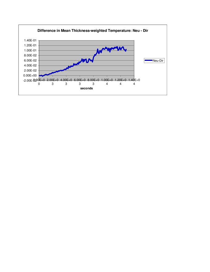
Figure 6: Difference in mean thickness-weighted temperature between Neumann (Neu) and Dirichlet (Dir) cases

Figure 6 shows the difference in the mean thickness-weighted temperatures. Just like in Section 5.2, Neumann boundary conditions always generate a colder current, and the difference between the average temperatures increases linearly with time.

Both weighted-temperature metrics (11) and (12) give results consistent with the finding for entrainment in Section 5.1.

5.4 Total heat transport

Figure 2 shows the initial temperature distribution for both currents. The coldest (red) part is at the bottom, and the warmest (blue) part at the top.

The total heat transport for each current was calculated as

$$R(t)=\int(T*u\cdot\textbf{n})\,dz$$ (13)

at each time-step. $R(t)$ is then normalized with the length of the current at that time step.

The finding is that, on average, the current with Neumann boundary conditions transports more than Dirichlet case, by $9.34\%$.

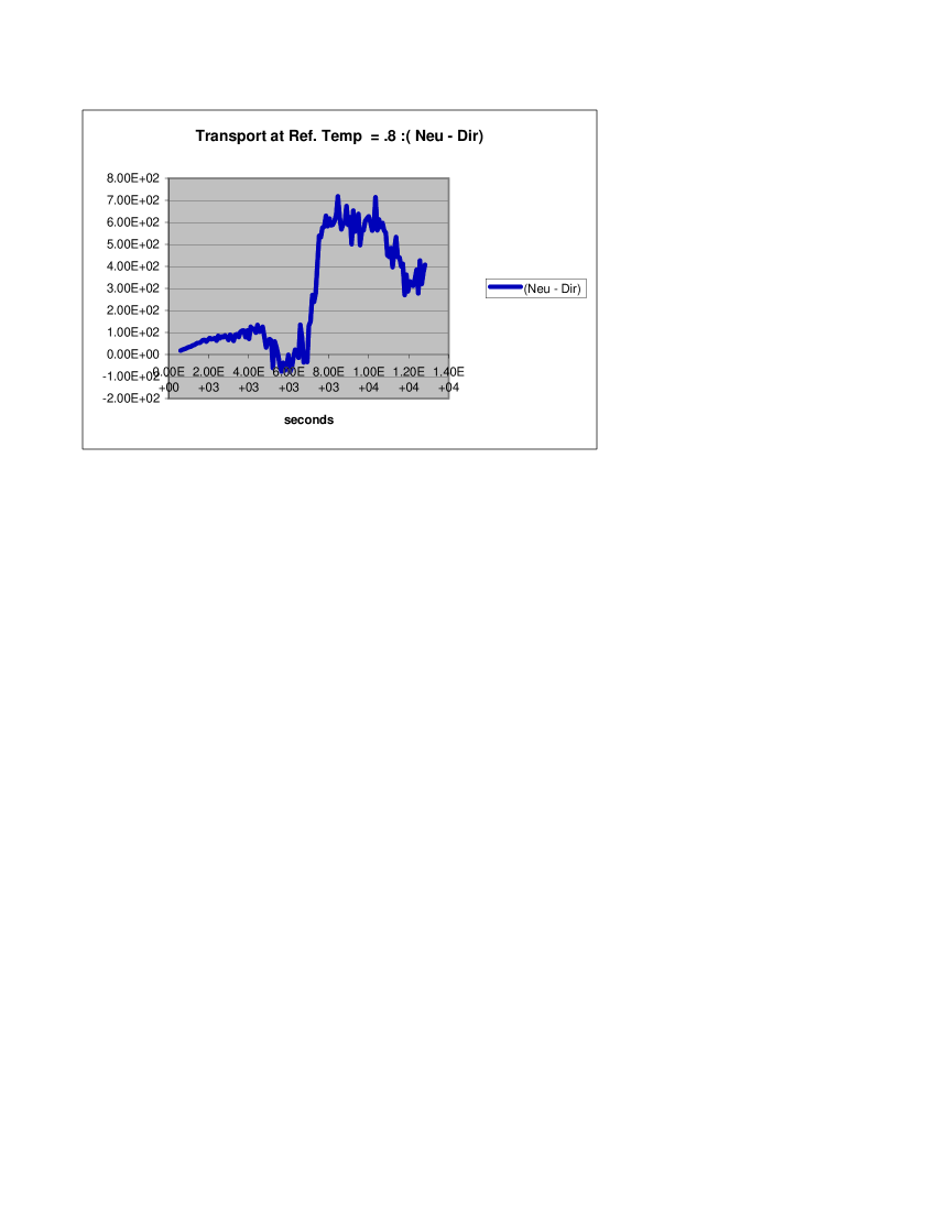
Figure 7: Difference in total temperature transport between Neumann and Dirichlet cases

Figure 7 shows a dramatic rise in the difference in transport between the two currents at about 6840 seconds (roughly 1/3 of the way down the domain); the head breaks down at roughly 10,000 seconds (real time).

5.5 Incremental heat transport

In the same experiment, repeated calls to the flux-volume calculations are done, changing the reference temperature each time. This allows the calculation of heat transport for different reference temperatures.

The data in Section 5.4 came from the standard reference temperature of $0.8$, which means that only fluid with nondimensional temperatures less than or equal to $0.8$ get into the calculation for $R(t)$ in equation $(13)$ above.

Figure 8 shows the heat transport spectrum plotted for the current with Neumann boundary conditions, at reference temperatures $0.8,0.7,0.5,0.3$ and $0.1$. Notice that temperature transport increases as the reference temperatures increases. This is because the higher the reference temperature, the greater the part of the current that it encompasses. Indeed, the standard reference temperature of $0.8$ encompasses all temperatures from $0.0$ to $0.8$. On the other hand, a reference temperature of $0.7$ encompasses only temperatures from $0.0$ to $0.7$. The Dirichlet boundary conditions give a similar spectrum.

The difference in thermal transport between reference temperatures $0.5$ and $0.7$ is calculated, and this gives an estimate of the way temperature is transported from the top (warmest part) towards the bottom (coolest part) of the current. This is equivalent to calculating $R(t)$ in equation $(13)$ in the previous section, but only for nondimensional temperatures $0.5\leq T\leq 0.7$.

The same calculation is repeated for the middle temperature range (from $0.3$ to $0.5$) and low range (from $0.1$ to $0.3$).

The finding here is that, at the middle range, (from $0.3$ to $0.5$), the Dirichlet case transports more by $28.63\%$ (see Fig. 9). At the high range (from $0.5$ to $0.7$), Dirichlet continues to transport more, by $11.59\%$, on average. However, at the low temperature range (from $0.1$ to $0.3$), Neumann boundary conditions now give a bigger transport, by more than $7.37\%$. This suggests that there is a major difference in the way the two currents transport at medium temperatures, and the difference in the incremental transport increases almost linearly with time.

6 Conclusions

Gravity currents with two types of boundary conditions on the bottom continental shelf, Neumann (insulation) and Dirichlet (fixed temperature), were investigated. The major finding is that the incremental temperature transport metric best differentiates the two currents.

It was noted that the effect is most significant at the medium temperature range ($0.3$ - $0.5$), where the difference was $28.63\%$. In this range, the current with Dirichlet boundary conditions transported more heat.

The other findings (in order of greatest differences) are: The entrainment $E(t)$ metric also differentiates the two currents significantly, showing that Dirichlet boundary conditions cause a current to entrain by about $14.21\%$ more. The incremental temperature transport at the high temperature range showed that the Dirichlet case transports by $11.59\%$ more. The mean thickness-weighted temperature showed that Neumann boundary conditions yield a current that is by about ${9.36\%}$ colder. The transport at standard reference temperature showed that the Neumann case transports by $9.34\%$ more. The incremental transport at the low temperature range showed that the Neumann boundary conditions cause about $7.37\%$ greater transport. Finally, the velocity-weighted temperature showed that the Neumann case yields a current that is by about $5.61\%$ colder.

Thus, the observed temperature distribution of the gravity current results from a complex interaction of temperature being transported from below, and ambient water being entrained from above. The present study is just a first step toward a better understanding of this complex interaction. In particular, it is found that there can be significant differences in the entrainment and transport of gravity currents when the most popular Neumann boundary conditions, or the less popular Dirichlet boundary conditions are used on the bottom continental shelf.

A better understanding of the impact of both velocity and temperature boundary conditions on entrainment and transport in gravity currents is needed. In particular, slip-with-friction boundary conditions for the velocity on the bottom continental shelf appear as a more appropriate choice. Robin boundary conditions for the temperature on the bottom should also be investigated. Different outflow velocity and temperature boundary conditions (such as “do-nothing”) could also yield more physical results, essential in an accurate long time integration of the gravity current. All these issues will be investigated in futures studies.

Acknowledgement. This work was partly supported by AFOSR grants F49620-03-1-0243 and FA9550-05-1-0449, and NSF grants DMS-0203926, DMS-0209309, DMS-0322852, and DMS-0513542. The authors would like to thank Professors Xiaofan Li and Dietmar Rempfer for their helpful suggestions, and the two anonymous reviewers for their insightful comments and suggestions which improved the paper.

Figure 1: Set-up

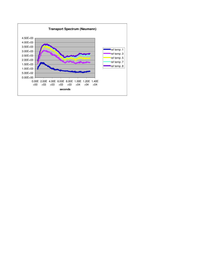
Figure 8: Transport spectrum for Neumann case for various reference temperatures

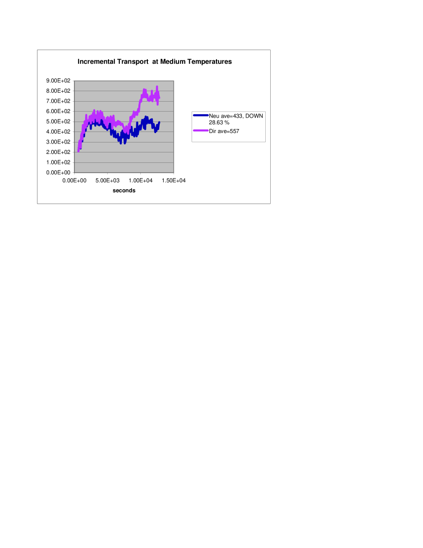
Figure 9: Incremental transport across medium temperature range $(0.3-0.5)$

References

- [1] Simpson, J. E., 1982: Gravity currents in the laboratory, atmosphere, and the ocean. Ann. Rev. Fluid Mech., 14, 213-234.
- [2] Cenedese, C., J. A. Whitehead, T. A. Ascarelli and M. Ohiwa, 2004: A Dense Current Flowing Down a Sloping Bottom in a Rotating Fluid. J. Phys. Oceanogr., 34, 188-203.
- [3] Smith, P. C., 1975: A Streamtube Model for Bottom Boundary Currents in the Ocean. Deep-Sea Res., 22, 853-873.
- [4] Killworth, P. D., 1977: Mixing on the Weddell Sea Continental Slope. Deep-Sea Res., 24, 427-448.
- [5] Özgökmen, T., P. Fischer, J. Duan and T. Iliescu, 2004: Three-Dimensional Turbulent Bottom Density Currents From a High-Order Nonhydrostatic Spectral Element Method. J. Phys. Oceanogr., 34, 2006-2026.
- [6] Heggelund, Y., F. Vikebo, J. Berntsen, and G. Furnes, 2004: Hydrostatic and non-hydrostatic studies of gravitational adjustment over a slope. Continental Shelf Research, 24 (18), 2133-2148.
- [7] Shapiro, G. I. and A. E. Hill, 1997: Dynamics of Dense Water Cascades at the Shelf Edge J. Phys. Oceanogr., 27 (11), 2381-2394.
- [8] Hallworth, M. A., H. E. Huppert, and M. Ungarish, 2001: Axisymmetric gravity currents in a rotating system: experimental and numerical investigations, J. Fluid Mech., 447, 1-29.
- [9] Özgökmen, T. and E. P. Chassignet, 2002: Dynamics of Two-Dimensional Turbulent Bottom Gravity Currents. J. Phys. Oceanogr., 32,1460-1478 .
- [10] Özgökmen, T., P. Fischer, J. Duan and T. Iliescu, 2004: Entrainment in bottom gravity currents over complex topography from three-dimensional nonhydrostatic simulations. Geophysical Research Letters, 31, L12212.
- [11] Härtel, C., L. Kleiser, M. Michaud, C. F. Stein, 1997: A direct numerical simulation approach to the study of intrusion fronts. J. Engrg. Math., 32 (2-3), 103-120.
- [12] Ockendon, J., S. Howison, A. Lacey, and A. Movchan, 1999: Applied Partial Differential Equations . Oxford University Press, pp. 147.
- [13] Murray, S. P. and W. E. Johns, 1997: Direct observations of seasonal exchange through the Bab el Mandep Strait, Geophys. Res. Lett., 24, 2557-2560.
- [14] Özgökmen, T. M., P. F. Fischer, and W. E. Johns, 2006: Product water mass formation by turbulent density currents from a high-order nonhydrostatic spectral element model, Ocean Modelling, 12, 237-267.
- [15] Cushman-Roisin, B. 1994: Introduction to Geophysical Fluid Dynamics. Prentice Hall Oxford University Press, pp. 10.
- [16] Ledwell, J. R., A. J. Watson, and C.S. Law, 1993: Evidence for slow mixing across the pycnocline from an open-ocean tracer-release experiment. Nature, 364, 701-703.
- [17] Maday, Y. and A. T. Patera, 1989: State of the Art Surveys in Computational Mechanics. ASME, New York, ed. by A.K. Noor, pp. 71-143.
- [18] Fischer, P. F. and J. S. Mullen, 2001: Filter-Based Stabilization of Spectral Element Methods. Comptes rendus de l’Academie des Science Paris, t. 332, - Serie I - Analyse Numerique, 38 pp. 265-270.
- [19] Perot, J. B., 1993: An analysis of the fractional step method. J. Comp. Physics, 108 pp. 310-337.
- [20] Maday, Y., A. T. Patera, and E. M. Ronquist, 1990: An operator-integration-factor splitting method for time-dependent problems: application to incompressible fluid flow. J. Sci. Comput., 5(4) pp. 51-58.
- [21] Fischer, P. F., 1997: An Overlapping Schwarz Method for Spectral Element Solution of the Incompressible Navier-Stokes Equations. J. Comp. Phys. , 133, pp. 84-101.
- [22] Fischer, P. F., N. I. Miller, and H. M. Tufo, 2000: An Overlapping Schwarz Method for Spectral Element Simulation of Three-Dimensional Incompressible Flows. Parallel Solution of Partial Differentail Equations . Springer-Verlag, ed. by P. Bjorstad and M. Luskin, pp 159-181.
- [23] Fischer, P. F., 1996: Parallel multi-level solvers for spectral element methods. Proceedings of Intl. Conf. on Spectral and High-Order methods ’95, Houston, TX, A. V. Ilin and L. R. Scott, Eds.
- [24] Tufo, H. M., and P. F. Fischer, 1999: Terascale Spectral Element Algorithms and Implementations. Gordon Bell Prize submission, Proceedings of ACM/IEEE SC99 Conf. on High Performance Networking and Computing. IEEE Computer Soc., CDROM.
- [25] Renardy, M. 1997: Imposing ’No’ Boundary Condition at Outflow: Why Does it Work? Int. J. Num. Meth. Fluids, 24, 413-417.
- [26] Layton, W. 1999: Weak Imposition of “No-Slip” Conditions in Finite Element Methods Comput. Math. Appl., 38(5), 129-142.
- [27] Liakos, A. 1999: Weak imposition of boundary conditions in the Stokes and Navier-Stokes equation PhD thesis, Univ. of Pittsburgh.
- [28] John, V. 2002: Slip with friction and penetration with resistance boundary conditions for the Navier–Stokes equations–numerical tests and aspects of the implementation J. Comp. Appl. Math., 147(2), 287-300.
- [29] Härtel, C., E. Meiburg, and F. Necker, 2000: Analysis and direct numerical simulation of the flow at a gravity-current head. Part 1. Flow topology and front speed for slip and no-slip boundaries. J. Fluid Mech., 418, 189-212.
- [30] Rempfer, D. On Boundary Conditions for Incompressible Navier-Stokes Problems. To appear in Applied Mechanics Reviews. (2005)
- [31] Morton, B. R., G. I. Taylor, and J. S. Turner, 1956: Turbulent gravitational convection from maintained and instantaneous sources. Proc. R. Soc. Lond., A 234, 1-23.
- [32] Baringer, M. O., and J. F. Price, 1997: Mixing and spreading of the Mediterranean outflow. J. Phys. Oceanogr., 27, 1654-1677.