Phase-dependent light propagation in atomic vapors

Abstract

Light propagation in an atomic medium whose coupled energy levels form a $\diamondsuit$-configuration exhibits a critical dependence on the input conditions. Depending on the relative phase of the input light fields, the response of the medium can be dramatically modified and switch from opaque to semi-transparent. These different types of behaviour are caused by the formation of coherences due to interference in the atomic excitations. Alkali-earth atoms with zero nuclear spin are ideal candidates for observing these phenomena which could offer new perspectives in control techniques in quantum electronics.

I Introduction

Experimental evidence has demonstrated that the nonlinear optical properties of laser-driven atomic gases exhibit counter-intuitive features with promising applications. A peculiarity of these media is the possibility to manipulate their internal and external degrees of freedom with a high degree of control. Recently the control of the internal dynamics in an atomic vapor by means of electromagnetically induced transparency (EIT) EIT was demonstrated for the generation of four-wave mixing dynamics Harris04 and of controlled quantum pulses of light Harris05 ; Lukin05 . Zeeman coherence has also been used to induce phase dependent amplification without inversion in Samarium vapors Nottelmann93 and in HeNe mixtures Peters96 . In another experiment, the interplay of internal and external degrees of freedom in an ultracold atomic gas by means of recoil-induced resonances RIR was used to achieve waveguiding of light Prentiss05 . From this perspective, it is important to identify further possible control parameters on the atomic dynamics for the manipulation of the non-linear optical response of the medium.

Recent studies have been focusing on the dynamics of light interacting with atoms featuring coupled energy levels in a so-called ’closed-loop’ configuration Buckle86 ; Kosachiov92 . In this configuration a set of atomic states is (quasi-) resonantly coupled by laser fields so that each state is connected to any other via two different paths of coherent photon-scattering. As a consequence, the relative phase between the transitions critically influences dynamics Buckle86 and steady states Kosachiov92 ; Korsunsky99 ; Morigi02 . Applications of closed-loop configurations to nonlinear optics have featured double-$\Lambda$ systems where two stable or metastable states are -each- coupled to two common excited states. A rich variety of nonlinear optical phenomena has been predicted Korsunsky99 ; PhaseoniumRev ; Wilson-Gordon and experimentally observed VandenHeuwell ; Nottelmann93 ; Peters96 ; Windholz96 ; Harris00 ; Harris04 ; Windholz99 ; Windholz04 . In Windholz04 , in particular, it has been shown experimentally that the properties of closed-loop configurations can be used to correlate electromagnetic fields with carrier frequency differences beyond the GHz regime. Moreover, coherent control based on the relative phase in closed-loop configuration has been proposed in the context of quantum information processing Sola05 .

Figure 1: Electronic transitions of the $\diamondsuit$-configuration. Each transition $|i\rangle\to|j\rangle$ is resonantly driven by a laser field at frequency $\nu_{ij}$. Here, $|g\rangle$ is the ground state, $|1\rangle$ and $|2\rangle$ the intermediate states, which decay into the ground state at rates $\gamma_{1g}$ and $\gamma_{2g}$, respectively, and $|e\rangle$ the excited state, which decays with rates $\gamma_{e1}$ and $\gamma_{e2}$ into the corresponding intermediate states. Each pair of levels is coupled by two paths of excitation, hence the dynamics depends critically on the relative phase between the paths. The coherent dynamics of the $\diamondsuit$-configuration is equivalent to that of the double-$\Lambda$ scheme, whereas the radiative instability of the atomic levels differs.

In this work we investigate the phase-dependent dynamics of light propagation in a medium of atoms whose energy levels are driven in a closed-loop configuration, denoted by the $\diamondsuit$ (diamond) scheme and depicted in Fig. 1. This configuration consists of four driven transitions where one ground state is coupled in a V-type structure to two intermediate states, which are in turn coupled to a common excited state in a $\Lambda$-type structure. It can be encountered, for instance, in (suitably driven) isotopes of alkali-earth atoms with zero nuclear spin AlkaliEarth . Although the coherent dynamics of $\diamondsuit$ schemes is equivalent to that of double-$\Lambda$ systems Buckle86 , the steady states of the two systems exhibit important differences due to the different relaxation processes Korsunsky99 ; Morigi02 .

The dynamics of light propagation in a medium of $\diamondsuit$-atoms is studied by integrating numerically the Maxwell-Bloch equations. We find that, depending on the input field parameters, the polarization along the medium can be drastically modified. The propagation dynamics may exhibit two metastable values of the relative phase, namely the values $0$ and $\pi$, corresponding to a semi-transparent and to an opaque medium, respectively. For different values of the initial phase, light propagation along the medium tends to one of these two values, depending on the input values of the driving amplitudes. These two types of the medium response are supported by the formation of atomic coherences leading to a minimization of dissipation by depleting the population of one or more atomic states. This phase dependent behavior, selected at the input by the operator, offers promising perspectives in control techniques in quantum electronics.

The article is organized as follows. In Sec. II the model is introduced and discussed. In Sec. III the results for the dynamics of light propagation, solved numerically from the equations reported in Sec. II.4, are reported and discussed in some parameter regimes. Conclusions and outlooks are reported in Sec. IV. The appendices present in detail equations and calculations at the basis of the model derived in Sec. II.

II The Model

We consider a classical field propagating in a dilute atomic gas along the positive $z$-direction. The field is composed of four optical frequencies $\nu_{1g}$, $\nu_{2g}$, $\nu_{e1}$ and $\nu_{e2}$, its complex amplitude is a function of time $t$ and position $z$ of the form

$${\bf E}(z,t)=\frac{1}{2}\sum_{i,j}\mathcal{E}_{ij}(z,t){\bf e}_{ij}\text{e}^{-i(\nu_{ij}t-k_{ij}z+\phi_{ij}(z,t))}+{\rm c.c.},$$ (1)

where $k_{ij}$ denotes the wave vector and ${\bf e}_{ij}$ the polarization of the frequency component $\nu_{ij}$. The input field enters the medium at $z=0$, and the effect of coupling to the medium is accounted for in the $z$ dependence of the amplitude $\mathcal{E}_{ij}(z,t)$ and phase $\phi_{ij}(z,t)$ whose variations in position and time are slow with respect to the wavelengths $\lambda_{ij}=2\pi/k_{ij}$ and the oscillation periods $T=2\pi/\nu_{ij}$, respectively. The atomic gas is very dilute and we can assume that the atoms interact with the fields individually. In particular, each field component at frequency $\nu_{ij}$ drives (quasi-) resonantly the electronic transition $|{i}\rangle\to|{j}\rangle$ of the atoms in the medium, such that the atomic levels are coupled in a $\diamondsuit$-shaped configuration.

The relevant atomic transitions and the coupling due to the lasers are displayed in Fig. 1. The ground state $|{g}\rangle$ is coupled to the intermediate states $|{1}\rangle$, $|{2}\rangle$ at energies $\hbar\omega_{1},\hbar\omega_{2}$ by transitions with dipole moments ${\bf d}_{1g}=\langle{1}|{\bf d}|{g}\rangle$ and ${\bf d}_{2g}=\langle{2}|{\bf d}|{g}\rangle$, respectively. The intermediate states decay back into the ground state at decay rates $\gamma_{1g}$ and $\gamma_{2g}$. The intermediate states are also coupled to the excited state $|{e}\rangle$ at an energy $\hbar\omega_{e}$ with respect to the ground state $|{g}\rangle$, by the dipole transitions ${\bf d}_{e1}=\langle{e}|{\bf d}|{1}\rangle$, ${\bf d}_{e2}=\langle{e}|{\bf d}|{2}\rangle$. The excited state $|e\rangle$ decays into states $|1\rangle$ and $|2\rangle$ at rates $\gamma_{e1}$ and $\gamma_{e2}$, respectively. A similar configuration of levels can be found in isotopes of alkali atoms with zero nuclear spin AlkaliEarth .

The light fields propagating through the dilute atomic sample will induce a macroscopic polarization in the atoms. This polarization will depend on intensities and phases of the light fields. The polarization, in turn, will affect absorption and refraction of the light fields, altering their propagation. Below we introduce the equations for field propagation and the corresponding atomic dynamics.

II.1 Equations for field propagation

We denote by ${\bf P}(z,t)$ the macroscopic polarization induced in the atomic gas

$${\bf P}(z,t)=n\operatorname{Tr}\{{\bf\hat{d}}\sigma(z,t)\}$$ (2)

where ${\bf\hat{d}}$ is the dipole operator, $n$ is the density of the medium, which we assume to be zero for $z<0$ and uniform for $z>0$, and $\sigma(z,t)$ is the atomic density matrix at time $t$ and position $z$, which has been obtained by tracing out the other external degrees of freedom. Details of the underlying assumptions at the basis of Eq. (2) are discussed in Appendix A.

We decompose the polarization ${\bf P}(z,t)$ into slowly- and fast-varying components, namely

$${\bf P}(z,t)=\frac{1}{2}\sum_{i,j}\mathcal{P}_{ij}(z,t){\bf e}_{ij}\text{e}^{-i(\nu_{ij}t-k_{ij}z+\phi_{ij}(z,t))}+{\rm c.c.},$$ (3)

whereby the complex amplitudes $\mathcal{P}_{ij}$ and the phases $\phi_{ij}$ vary slowly as a function of position and time. We consider the parameter regime where the driving fields are sufficiently weak so that the generation of higher-order harmonics can be neglected. By comparing Eqs. (2) and (3), the amplitudes $\mathcal{P}_{ij}$ can be expressed in terms of the elements of the atomic density matrix $\sigma$,

$$\mathcal{P}_{ij}=2n\mathcal{D}_{ij}\sigma_{ij}e^{i(\nu_{ij}t-k_{ij}z+\chi_{ij})}$$ (4)

where $\sigma_{ij}=\langle{i}|\sigma|{j}\rangle$. We have expressed the dipole moments in direction of the electric field polarization as ${\bf e}_{ij}\cdot{\bf d}_{ji}=\mathcal{D}_{ij}{\rm e}^{-{\rm i}\theta_{ij}}$, thereby separating the complex amplitudes $\mathcal{P}_{ij}$ into modulus and phase. Here, the term $\mathcal{D}_{ij}$ is real, $\theta_{ij}$ are the dipole phases ($\theta_{ij}=-\theta_{ji}$), and

$$\chi_{ij}(z,t)=\phi_{ij}(z,t)-\theta_{ij}$$ (5)

is the sum of the slowly-varying field phases $\phi_{ij}(z,t)$ and the dipole phases $\theta_{ij}$.

Using definitions (1) and (3) and applying a coarse-grained description in time and space, the Maxwell equations simplify to a set of propagation equations for each of the slowly-varying components of the laser and polarization fields QScully

$$\frac{\partial\mathcal{E}_{ij}}{\partial z}+\frac{1}{c}\frac{\partial\mathcal{E}_{ij}}{\partial t} =-\frac{\nu_{ij}}{2\>\epsilon_{0}\>c}{\rm Im}\{\mathcal{P}_{ij}(\mathcal{E}_{kl},\phi_{kl})\},$$ (6)

$$\frac{\partial\phi_{ij}}{\partial z}+\frac{1}{c}\frac{\partial\phi_{ij}}{\partial t} =-\frac{\nu_{ij}}{2\>\epsilon_{0}\>c}\frac{1}{\mathcal{E}_{ij}}{\rm Re}\{\mathcal{P}_{ij}(\mathcal{E}_{kl},\phi_{kl})\},$$ (7)

which are defined for $z>0$. Here, each amplitude $\mathcal{E}_{ij}$ and phase $\phi_{ij}$ is coupled via the corresponding polarization $\mathcal{P}_{ij}$ to all other field amplitudes and phases.

We rescale the propagation equations using the dimensionless length and time

$$\xi=\kappa_{1g}z,~{}~{}~{}\tau=c\>\kappa_{1g}t.$$ (8)

Here $\kappa_{1g}$ is the absorption coefficient

$$\kappa_{1g}=n\frac{1}{\gamma_{1g}}\frac{\nu_{1g}\mathcal{D}_{1g}^{2}}{c\epsilon_{0}\hbar}$$

such that $1/\kappa_{1g}$ determines the characteristic length at which light driving the transition $|{g}\rangle\to|{2}\rangle$ penetrates a medium with density $n$. We denote the dimensionless field amplitudes by

$$\mathcal{G}_{ij}=\frac{\Omega_{ij}}{\gamma_{1g}}\frac{\mathcal{D}_{1g}^{2}\nu_{1g}}{\mathcal{D}_{ij}^{2}\nu_{ij}},$$ (9)

where

$$\Omega_{ij}(z,t)=\mathcal{D}_{ij}\mathcal{E}_{ij}(z,t)/\hbar$$ (10)

is the real valued Rabi frequency for the transition $|{i}\rangle\rightarrow|{j}\rangle$. In this notation the propagation Eqs. (6) and (7) reduce to the form

$$\frac{\partial\mathcal{G}_{ij}}{\partial\xi}+\frac{\partial\mathcal{G}_{ij}}{\partial\tau} =-\;{\rm Im}\{p_{ij}\},$$ (11)

$$\frac{\partial\phi_{ij}}{\partial\xi}+\frac{\partial\phi_{ij}}{\partial\tau} =-\;\frac{1}{\mathcal{G}_{ij}}\;{\rm Re}\{p_{ij}\},$$ (12)

where

$$p_{ij}(\xi,\tau)=\sigma_{ij}\text{exp}\left[i\left(\frac{\nu_{ij}}{c\;\kappa_{1g}}\tau-\frac{k_{ij}}{\kappa_{1g}}\xi+\chi_{ij})\right)\right]\;$$ (13)

denotes the atomic density matrix elements in a rotated reference frame. In the remainder of this paper we consider laser field geometries where $|{1}\rangle$ and $|{2}\rangle$ are states of the same hyperfine multiplet so that $\nu_{1g}\simeq\nu_{2g}$ and $\nu_{e1}\simeq\nu_{e2}$.

II.2 Atomic dynamics

The time evolution of the density matrix $\sigma(z,t)$ for the atomic internal degrees of freedom at position $z>0$ is governed by the master equation

$$\dot{\sigma}=\frac{1}{{\rm i}\hbar}\left[H(z,t),\sigma\right]+\mathcal{L}\sigma.$$ (14)

where $z$ is a classical variable. Equation (14) is obtained by tracing out the degrees of freedom of momentum and of position in the transverse plane, in the limit in which the medium is homogeneously broadened and the atoms are sufficiently hot and dilute such that their external degrees of freedom can be treated classically. Details of the assumptions at the basis of Eq. (14) are reported in Appendix A. Here the Hamiltonian

$$H(z,t) = \sum_{j=e,1,2,g}\hbar\omega_{j}|{j}\rangle\langle{j}|$$

$$- \frac{\hbar}{2}\sum_{j=1,2}\Bigl{(}\Omega_{jg}(z,t)\;e^{-i(\nu_{jg}t-k_{jg}z+\chi_{jg}(z,t))}\;|{j}\rangle\langle{g}|$$

$$+\Omega_{ej}(z,t)\;e^{-i(\nu_{ej}t-k_{ej}z+\chi_{ej}(z,t))}\;|{e}\rangle\langle{j}|+{\rm H.c.}\Bigr{)}$$

describes the coherent dynamics of the internal degrees of freedom, and it depends on $z$ through the (real-valued) Rabi frequency $\Omega_{ij}(z,t)$ given in Eq. (10), and through the field and dipole phases, Eq. (5).

The states $|{1}\rangle,|{2}\rangle$ and $|{e}\rangle$ are unstable and decay radiatively with rates $\gamma_{1g}$, $\gamma_{2g}$ and $\gamma_{e}=\gamma_{e1}+\gamma_{e2}$, respectively. The relaxation processes are described by

$$\mathcal{L}\sigma = \!\!\sum_{j=1,2}\frac{\gamma_{jg}}{2}\left(2|{g}\rangle\langle{j}|\sigma|{j}\rangle\langle{g}|-|{j}\rangle\langle{j}|\sigma-\sigma|{j}\rangle\langle{j}|\right)$$ (16)

$$+ \!\!\!\!\sum_{j=1,2}\!\!\frac{\gamma_{ej}}{2}\left(2|{j}\rangle\langle{e}|\sigma|{e}\rangle\langle{j}|-|{e}\rangle\langle{e}|\sigma-\sigma|{e}\rangle\langle{e}|\right),$$

where the recoil due to spontaneous emission is neglected since the motion is treated classically. In the remainder of this paper we assume a symmetrical decay of the excited level, $\gamma_{e1}=\gamma_{e2}=\gamma_{e}/2$.

We note that the transitions $|g\rangle\to|j\rangle$ ($j=1,2$) are saturated when $\Omega_{jg}\geq\gamma_{jg}.$ Correspondingly, the upper transitions $|j\rangle\to|e\rangle$ are saturated when $\Omega_{ej}\geq\gamma_{e}+\gamma_{jg}.$ For later convenience, we introduce

$$\mathcal{\tilde{G}}_{ej}=\frac{\mathcal{G}_{ej}}{1+\gamma_{e}/\gamma_{jg}},$$ (17)

which explicitly shows the scalings of the upper field amplitudes with the corresponding decay rates.

II.3 The relative phase

In so-called closed-loop configurations, like the $\diamondsuit$ scheme, transitions between each pair of electronic levels are characterized by -at least- two excitation paths, involving different intermediate atomic levels Kosachiov92 ; PhaseoniumRev . In the $\diamondsuit$ scheme the relative phase between these excitation paths critically determines the solution of the master equation, and hence the atomic response during propagation. The role of the relative phase in the atomic response is better unveiled by moving to a suitable reference frame for the atomic evolution, which is defined when all amplitudes $\mathcal{E}_{ij}$ are nonzero.

We denote by $\rho$ the density matrix in this reference frame, obeying the master equation

$$\dot{\rho}=\frac{1}{i\hbar}\left[\tilde{H},\rho\right]+\mathcal{L}\rho.$$ (18)

In this reference frame the Hamiltonian (II.2) is transformed to Buckle86 ; Morigi02

$$\tilde{H} = \hbar\Delta_{e}|{e}\rangle\langle{e}|+\hbar\Delta_{1}|{1}\rangle\langle{1}|+\hbar\Delta_{2}|{2}\rangle\langle{2}|$$

$$- \frac{\hbar}{2}\left(\Omega_{e1}\,|{e}\rangle\langle{1}|+\Omega_{e2}\,{\rm e}^{{\rm i}\Theta(z,t)}\,|{e}\rangle\langle{2}|\right.$$

$$\left.+\Omega_{1g}\,|{1}\rangle\langle{g}|+\Omega_{2g}\,|{2}\rangle\langle{g}|+{\rm H.c.}\right),$$

with the detunings

$$\Delta_{1} =\omega_{1}-\nu_{1g},$$ (20)

$$\Delta_{2} =\omega_{2}-\nu_{2g},$$ (21)

$$\Delta_{e} =\omega_{e}-\nu_{e1}-\nu_{1g}.$$ (22)

The Hamiltonian (II.3) exhibits an explicit dependence on the phase

$$\Theta(z,t)=\Delta\nu\;t-\Delta k\;z+\Delta\chi(z,t).$$ (23)

where

$$\Delta\nu =\nu_{e1}+\nu_{1g}-\nu_{2g}-\nu_{e2},$$ (24)

$$\Delta k =k_{e1}+k_{1g}-k_{2g}-k_{e2},$$ (25)

$$\Delta\chi(z,t) =\chi_{e1}(z,t)+\chi_{1g}(z,t)-\chi_{e2}(z,t)-\chi_{2g}(z,t),$$ (26)

with $\chi_{ij}$ as defined in Eq. (5).

The four-photon detuning $\Delta\nu$ results in a time-dependent phase, the wave-vector mismatch $\Delta k$ in a position dependent phase, and $\Delta\chi(z,t)$ comprises the relative dipole and field phases. In Korsunsky99 ; Morigi02 it has been discussed how $\Theta(z,t)$ affects the dynamics and steady state of the atom. The latter exists for $\Delta\nu=0$ and in the remainder of this article we assume

$$\Delta\nu=0,~{}\Delta k=0,$$

i.e., the atoms are driven at four-photon resonance and by copropagating laser fields, such that the wave vector mismatch is negligible. Hence, the phase

$$\Theta(z,t)=\Delta\chi(z,t)$$

depends solely on the relative dipole phase, which is constant, and on the relative phase of the propagating fields, which evolves according to the coupled Eqs. (11) and (12).

II.4 Propagation of the field amplitudes and phases

Having introduced the basic assumptions and definitions, we now report the equations for the propagation of the field amplitudes and phases in the $\diamondsuit$–medium, which are numerically solved in Sec. III. We relate the elements of the density matrix $\rho$ in the new reference frame with the elements $p_{ij}$ from eq. (13) by $\rho_{g1}=p_{g1}$, $\rho_{g2}=p_{g2}$, $\rho_{e1}=p_{e1}$, and

$$\rho_{e2}=p_{e2}\text{exp}\left(-{\rm i}\Theta\right).$$

The propagation equations for the light fields in the new reference frame can then be obtained from Eqs. (11)-(12) and take the form

$$\frac{\partial\mathcal{G}_{jg}}{\partial\xi^{\prime}}=-{\rm Im}\{\rho_{jg}\}\,,$$ (27)

$$\frac{\partial\phi_{jg}}{\partial\xi^{\prime}}=-\frac{{\rm Re}\{\rho_{jg}\}}{\mathcal{G}_{jg}}$$ (28)

for $j=1,2$ and

$$\frac{\partial\mathcal{G}_{e1}}{\partial\xi^{\prime}}=-{\rm Im}\{\rho_{e1}\}\,,$$ (29)

$$\frac{\partial\phi_{e1}}{\partial\xi^{\prime}}=-\frac{{\rm Re}\{\rho_{e1}\}}{\mathcal{G}_{e1}}\,,$$ (30)

$$\frac{\partial\mathcal{G}_{e2}}{\partial\xi^{\prime}}=-{\rm Im}\{\rho_{e2}e^{i\Theta}\}\,,$$ (31)

$$\frac{\partial\phi_{e2}}{\partial\xi^{\prime}}=-\frac{{\rm Re}\{\rho_{e2}e^{i\Theta}\}}{\mathcal{G}_{e2}}\,,$$ (32)

where we have introduced the variable

$$\xi^{\prime}=\xi+\tau.$$

These equations describe the evolution of field amplitudes and phases as a function of the atomic density matrix elements $\rho_{ij}$. In turn, the values of $\rho_{ij}$ depend on the field amplitudes and the relative phase $\Theta$ according to Eqs. (18) and (II.3). The propagation dynamics now can be investigated by solving the coupled Eqs. (18) and (27)-(32). The optical Bloch equations for the density matrix $\rho$ are presented in Appendix B.

In general, the density matrix elements entering Eqs. (27)-(32) are time dependent, i.e., $\rho=\rho(\tau)$. In this paper we consider the case of sufficiently long laser pulses, such that the characteristic time of change of amplitude and phase of the fields and the interaction time between light and atoms exceed the time scale in which the atom reaches the internal steady state. In this regime, we can neglect transient effects, and the density matrix elements entering Eq. (27)-(32) are the stationary solutions of Eq. (18) satisfying $\partial\rho/\partial t=0.$ This assumption allows us to neglect the time derivative in Eqs. (27)-(32), hence taking $\xi^{\prime}\approx\xi$.

The numerical study of the solutions of Eqs. (27)-(32) presented in this paper is restricted to certain parameter regimes that single out the role played by the phase and the radiative decay processes in the dynamics. In particular, we consider the situation where each atomic transition is driven at resonance, namely

$$\Delta_{i}=0,$$

for $i=1,2,e$. Moreover, we restrict ourselves to the regime where the fields are initially driving the corresponding transitions at saturation. This latter assumption is important to guarantee a finite occupation of the excited state $|e\rangle$, and thus to highlight the dependence of the dynamics on the relative phase $\Theta$.

During propagation, it may occur that one of the field amplitudes vanishes in just one point of the propagation variable $\xi^{\prime}$. When this happens, the relative phase $\Theta$ is not defined and its value has to be reset manually by imposing continuity of the trajectory, when integrating the field equations in amplitude and phase (see Eqs. (27)-(32)). The correctness of this procedure has been checked by comparing the results with those obtained by integrating the field equations for the real and imaginary parts of the complex field amplitudes.

III Light propagation in the $\Diamond$-medium

In this section we summarize some peculiar properties of the $\diamondsuit$-level scheme, which have been extensively discussed in Morigi02 . These properties provide an important insight into the propagation dynamics, which we study by solving numerically the Maxwell-Bloch Equations, Eqs. (18) and (27)-(32), in the regime where the input fields couple resonantly and saturate the corresponding electronic transitions, as described in Sec. II.4.

III.1 Symmetries of the $\diamondsuit$–level scheme

Figure 2: Level schemes onto which the $\diamondsuit$ configuration is mapped, if the lower field amplitudes, as well as the upper field amplitudes, are equal. For $\Theta=\pi$, the $\diamondsuit$ system imitates a V-configuration (a). Mapping to the $\Xi$-configuration, (b), is obtained for $\Theta=0$ and when $|e\rangle$ is metastable. Similarly, the mapping to the $\Lambda$-configuration (c) is obtained for $\Theta=0$ and metastable intermediate states.

Before entering the detailed discussion of the numerical results, it is instructive to review some basic properties of the $\diamondsuit$–level scheme, which significantly affect its response to light-propagation. Special symmetries of this configuration are encountered when the laser amplitudes, resonantly driving the upper (lower) transitions, are initially equal, namely when

$$\mathcal{G}_{e1}=\mathcal{G}_{e2}=\mathcal{G}_{e}$$ (33)

$$\mathcal{G}_{1g}=\mathcal{G}_{2g}=\mathcal{G}_{g}.$$ (34)

In this regime, the Hamiltonian (II.3) substantially simplifies for some values of the phase. In particular, for

$$\Theta=0,\pi$$

(modulus $2\pi$) the dynamics can be mapped to those of well-known three–level schemes Morigi02 . Insight is gained by studying Hamiltonian (II.3) in a convenient orthogonal basis set of atomic states.

For $\Theta=\pi$, Hamiltonian (II.3) describes coherent coupling within the orthogonal subspaces $\{|{g}\rangle,|{\Psi_{12}^{+}}\rangle\}$ and $\{|{e}\rangle,|{\Psi_{12}^{-}}\rangle\}$, where $|{\Psi_{12}^{\pm}}\rangle=\left[|{1}\rangle\pm|{2}\rangle\right]/\sqrt{2}$. These subspaces are decoupled: state $|{\Psi_{12}^{+}}\rangle$ is decoupled from $|e\rangle$ and $|{\Psi_{12}^{-}}\rangle$ from $|g\rangle$ by destructive interference. Spontaneous decay eventually pumps the atom into the subspace $\{|{g}\rangle,|{\Psi_{12}^{+}}\rangle\}$, see Fig. 2(a). Hence, in the stationary regime the excited state is depleted and the atomic levels which scatter light can be mapped onto a V-level scheme.

For $\Theta=0$ and under condition (33), (34), the Hamiltonian (II.3) can be written in two equivalent ways: It can describe coherent scattering among the orthogonal levels $\{|1\rangle,|\Psi_{eg}^{+}\rangle,|2\rangle\}$, forming a $\Lambda$-configuration, while state $|{\Psi_{eg}^{-}}\rangle$ is decoupled, or alternatively, it can describe coherent scattering among the orthogonal levels $\{|g\rangle,|\Psi_{12}^{+}\rangle,|e\rangle\}$, forming a $\Xi$-level scheme, while state $|{\Psi_{12}^{-}}\rangle$ is decoupled. Here, $|{\Psi_{eg}^{\pm}}\rangle$ are symmetric and antisymmetric superpositions of the states $|e\rangle$ and $|g\rangle$. However, if spontaneous decay is included, the two schemes are not equivalent. The relaxation processes select one configuration over the other depending on the stability of state $|{\Psi_{eg}^{-}}\rangle$, which decays at a rate $\gamma_{e}$, with respect to the stability of state $|{\Psi_{12}^{-}}\rangle$, which decays at a rate $\gamma_{1g}+\gamma_{2g}$. It is then important to introduce the parameter

$$\alpha=\frac{\gamma_{e}}{\gamma_{1g}+\gamma_{2g}}$$ (35)

which is the ratio between the decay rates of the two decoupled states, or, equivalently, the ratio between the decay of the excited and intermediate states. Hence, for $\alpha\ll 1$ (i.e. the excited state is longer lived than the intermediate ones), $|{\Psi_{12}^{-}}\rangle$ is essentially empty, and the effective dynamics can be mapped to a $\Xi$-level scheme, see Fig. 2(b). For $\alpha\gg 1$ instead (i.e. the intermediate state is longer lived than the excited one), $|{\Psi_{eg}^{-}}\rangle$ is empty, and the effective dynamics can be mapped to a $\Lambda$-level scheme, see Fig. 2(c). Hence, if the ratio $\alpha$ is sufficiently different from unity, the dynamics of the $\diamondsuit$-scheme can be mapped to three-level schemes and leads to coherent population trapping (CPT) EIT in the stationary state. In the $\Lambda$ case ($\alpha\gg 1$), a large coherence between the intermediate states is observed as reported in the transient dynamics of pulse propagation in a medium of $\diamondsuit$-atoms VandenHeuwell . Here, for some parameter regimes one can observe population inversion at steady state on the transition $|{g}\rangle\to|{1}\rangle,|{2}\rangle$ Morigi02 . In the $\Xi$ case ($\alpha\ll 1$), a macroscopic coherence between ground and excited states is created. For some parameter regimes one can observe population inversion at steady state on the transition $|{1}\rangle,|{2}\rangle\to|{e}\rangle$ Stroud76 .

These properties have important consequences for the propagation dynamics. We note that for $\Theta=0,\pi$ the components of the polarizations ${\rm Re}(\rho_{1g})$, ${\rm Re}(\rho_{2g})$, ${\rm Re}(\rho_{1e})$, ${\rm Re}(\rho_{2e}\exp({\rm i}\Theta))$ vanish. This means that the field phases remain constant upon propagation in agreement with Eqs. (28), (30) and (32). Hence, if at the input

$$\Theta(\xi=0)=0,\,\pi,$$ (36)

then

$$\frac{\partial\Theta}{\partial\xi}=0$$ (37)

and the relative phase remains constant during propagation along the medium. We recall that for $\Theta=\pi$ we observe a V-type dynamics (from now on denoted as destructive interference) and for $\Theta=0$ metastable CPT on a $\Xi$ or $\Lambda$-scheme (from now on denoted as constructive interference). Hence, from these simple considerations we expect that for different values of the input phase and relaxation rates, energy will be dissipated at very different rates along the medium.

III.2 Destructive interference in the atomic excitations

For $\Theta(0)=\pi$ the atoms are perfectly decoupled from the upper fields independently of their intensity and the upper state is empty as described in III.1. Destructive interference makes the polarizations of the transitions between the intermediate and the upper states as well as the population of the excited state to vanish identically, i.e., $\rho_{e1}=\rho_{e2}=\rho_{ee}=0$ Morigi02 . Correspondingly, the dynamics of light propagation of the lower fields is expected to be that encountered in a medium of V-atoms.

Figure 3(a) displays the propagation dynamics along the medium for $\Theta(0)=\pi$ and equal initial field amplitudes, $\mathcal{G}_{ij}(0)=\mathcal{G}_{0}$. Here, one sees that the upper fields propagate through the medium as if it were transparent, keeping a constant value. The amplitudes of the lower fields display identical decays. Figure 3(b) presents the corresponding populations of the energy levels along the medium. The energy level $|e\rangle$ remains depleted while the intermediate states $|1\rangle$ and $|2\rangle$ maintain the same population as a function of $\xi$ corresponding to the fact that the lower fields decay identically along the medium. The value of ground and intermediate state populations is the saturation value of the corresponding dipole transition until about $\xi\sim 200$ when the lower fields $\mathcal{G}_{jg}(\xi)$ do not saturate the transition any longer. After this penetration length only the ground state is appreciably occupied. Note that these dynamics are independent of the upper field amplitudes, as they remain decoupled from the atoms.

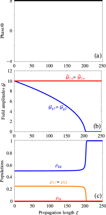
Figure 3: (color online) Propagation of the phase (a), field amplitudes (b) and the corresponding atomic state populations (c) for an input phase of $\Theta(0)=\pi$. Here, $\tilde{\mathcal{G}}_{e}$ is the rescaled amplitude as in Eq. (17). The phase is constant and the upper fields propagate unperturbed through the medium, while the excited state $|e\rangle$ remains depleted. The behavior is independent of $\mathcal{G}_{e}$ and $\gamma_{e}$ and thus of $\alpha$.

We can find an analytic expression for the dynamics shown in Fig. 3 and for the propagation length of the lower fields by solving the propagation equations (II.3) and (27)-(32) for $\Theta(0)=\Theta=\pi$. Setting $\mathcal{G}_{ej}=\mathcal{G}_{e}$ and $\mathcal{G}_{jg}=\mathcal{G}_{g}$, we obtain the equations for the dimensionless amplitudes

$$\frac{\partial\mathcal{G}_{g}}{\partial\xi} =-\frac{\mathcal{G}_{g}}{1+4\mathcal{G}_{g}^{2}},$$ (38)

$$\frac{\partial\mathcal{G}_{e}}{\partial\xi} =0.$$ (39)

Here the right hand side in Eq. (39) vanishes since ${\rm Im}\{\rho_{ij}(\Theta=\pi)\}=0$. Therefore, the relative phase $\Theta$ and the upper field amplitudes $\mathcal{G}_{e}$ are constant along the medium and the medium is transparent for the upper fields. Equation (38) is the equation for an electric field propagating in a medium of resonant dipoles so that the lower field amplitudes $\mathcal{G}_{g}$ decay during propagation at a rate that depends only on the value of $\mathcal{G}_{g}$ itself. In the case of large input intensities (see Fig. 3) a simple equation for $\mathcal{G}_{g}(\xi)$ is obtained AllenEberly

$$\mathcal{G}_{g}(\xi)=\sqrt{\mathcal{G}_{g}^{2}(0)-\xi/2}$$ (40)

allowing for an estimate of the penetration depth ($2\mathcal{G}_{g}^{2}(0)$) of the lower fields in the medium.

III.3 Constructive interference in the atomic excitations

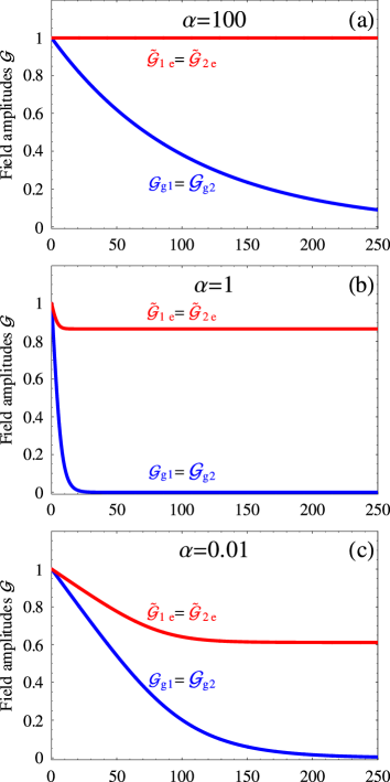
Figure 4: (color online) Field amplitudes as a function of the propagation length $\xi$ for input parameters $\Theta=0$, $\mathcal{\tilde{G}}_{e}=\mathcal{G}_{g}=1$ and different ratios between the decay rates: long lived intermediate states, $\alpha=100$, in (a), balanced decay rates, $\alpha=1$, in (b), and long lived excited state, $\alpha=0.01$, shown in (c). Correspondingly, the phase $\Theta=0$ remains constant along the medium (not shown). The rate of dissipation is critically determined by $\alpha$ and is slower for $\alpha$ sufficiently larger or smaller than unity.

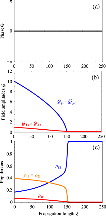
Figure 5: (color online) Propagation of phase (a), field amplitudes (b) and associated populations (c) for input parameters $\Theta=0$, $\mathcal{\tilde{G}}_{e}=1$, $\mathcal{G}_{g}=10$, and $\alpha=10$. Population inversion between the intermediate levels and the ground level is found along the medium until $\xi\sim 100$.

As discussed in section III.1, for $\Theta=0$ the response of the system is similar to that of a $\Xi$ or of a $\Lambda$ level scheme, depending on the ratio of the decay rates $\alpha$ in Eq. (35). Atomic coherences between either the intermediate states or the ground and excited state may form, and correspondingly the imaginary part of the polarizations may become very small, thus reducing dissipation.

Figure 4 displays the propagation dynamics along the medium for different values of the ratio $\alpha$ for $\Theta(0)=0$. For $\alpha\gg 1$ and $\alpha\ll 1$ the amplitudes decay slowly as a function of $\xi$, as expected from the formation of EIT-coherences. Figure 5 shows light propagation for the case when the initial conditions of the fields give rise to population inversion at steady state due to metastable CPT. We find that population inversion is maintained until $\xi\sim 100$ along the absorbing medium, but it gradually decreases, since the atomic coherences that are supporting CPT are not stable.

In the simulations of Figures 4 and 5, the lower (upper) field amplitudes remain equal during propagation. If we assume that $\mathcal{G}_{ej}=\mathcal{G}_{e}$ and $\mathcal{G}_{jg}=\mathcal{G}_{g}$ for all relevant $\xi$, then the propagation equations for the amplitudes reduce to

$$\frac{\partial\mathcal{G}_{e}}{\partial\xi} =-\frac{\mathcal{G}_{e}\;\mathcal{G}_{g}^{2}\;\alpha}{D_{0}}\;(1+2\alpha),$$ (41)

$$\frac{\partial\mathcal{G}_{g}}{\partial\xi} =-\frac{\mathcal{G}_{g}\;\alpha}{D_{0}}\;\left[\mathcal{G}_{g}^{2}+\alpha+2\alpha^{2}+\mathcal{G}_{e}^{2}\;(1+\alpha)\right],$$ (42)

with

$$D_{0} = \mathcal{G}_{e}^{4}\;(1+\alpha)+(1+4\mathcal{G}_{g}^{2})\;\alpha\;(\mathcal{G}_{g}^{2}+\alpha+2\alpha^{2})$$ (43)

$$+\mathcal{G}_{e}^{2}\;\left[\alpha\;(2+3\alpha)+\mathcal{G}_{g}^{2}\;(1+3\alpha+2\alpha^{2})\right]\,.$$

Equations (41) and (42) describe the dissipative propagation of the field amplitudes, and exhibit a nonlinear dependence on the amplitudes and the ratio $\alpha$ of the decay constants. Here, one can see that for different values of $\alpha$ the absorption lengths can vary by orders of magnitude. Limiting cases are found for $\alpha\to 0$, i.e. when the excited state is stable, and for $\alpha\to\infty$, i.e., when the intermediate states are stable. In these cases, the right hand sides of Eqs. (41) and (42) vanish, damping is absent, and light propagates through the medium as if it were transparent Footnote .

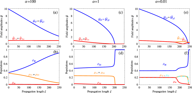
Figure 6: (color online) Propagation of fields (upper row) and corresponding atomic states populations (lower row) as a function of the propagation length and for different values of the excited state decay rate. The initial conditions are $\Theta(0)=0$, $\mathcal{G}_{g}(0)=10$ and $\tilde{\mathcal{G}}_{e}(0)=1$. Here, (a) and (b) correspond to the case $\alpha=100$, (c) and (d) to the case $\alpha=1$, and (e) and (f) to the case $\alpha=0.01$. In this latter case, the upper field amplitudes, $\tilde{\mathcal{G}}_{e1}$ and $\tilde{\mathcal{G}}_{e2}$, become different: energy is transferred from one field to the other, such that the amplitude of one increases while the other gradually vanishes. At this point, the phase $\Theta$ jumps to the value $\pi$, and energy is redistributed between the upper fields till they reach the same value. This behavior hints to an instability of the phase value $\Theta=0$, which seems to be triggered by numerical fluctuations of the values of the upper field amplitudes.

III.4 Stability of interference under amplitude fluctuations

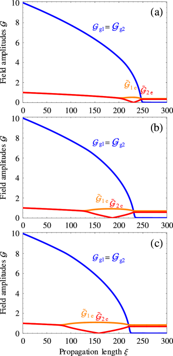
Figure 7: (color online) Study of the instability, shown in Fig. 6(e), as a function of different size of the upper field amplitude fluctuation $\delta\mathcal{G}_{e}$. The curves show the field amplitudes as a function or the propagation length $\xi$, for $\alpha=0.01$, $\mathcal{G}_{jg}(0)=\mathcal{G}_{g}=10$, $\mathcal{\tilde{G}}_{e1}(0)=1$ and $\mathcal{\tilde{G}}_{e2}(0)=1-\delta\mathcal{G}_{e}$ with (a) $\delta\mathcal{G}_{e}=10^{-16}$, (b) $\delta\mathcal{G}_{e}=10^{-12}$ and (c) $\delta\mathcal{G}_{e}=10^{-8}$.

In the cases discussed so far, the input phase is a constant of the propagation, and the amplitudes of the upper fields, as well as the amplitudes of the lower fields remain equal along the medium. We now address the question of stability of these configurations against phase and amplitude fluctuations.

Numerical investigations show that at $\Theta=\pi$ the V-level dynamics is robust against phase and amplitude fluctuations, from which we infer that this is a stable configuration. It should be remarked that the overall behavior is transient in that the medium dissipates the lower fields until (well inside the medium) the atoms are all found in the ground state.

The case $\Theta=0$ is more peculiar. In the cases discussed in Sec. III.3, energy is exchanged between upper and lower fields until the lower field amplitudes go below saturation. Then, the upper fields decouple as the population of the intermediate states becomes negligible. In order to study the long term dynamics of propagation, we now focus on the regime where the lower transitions are driven well above saturation and where we may expect different length scales for the propagation of the upper and lower fields.

Figure 6 displays propagation when the lower transitions are driven well above saturation for different values of $\alpha$. The dynamics observed in the $\alpha=1$ case separates the regimes corresponding to a $\Xi$-like response for $\alpha\ll 1$, and a $\Lambda$-like response for $\alpha\gg 1$. For the separating case of $\alpha=1$ in Fig. 6(c) and (d) we find that the damping of the lower fields below saturation is accompanied by a drop of the population from intermediate to ground states. For $\alpha=100$, shown in Fig. 6(a) and (b) propagation is characterized by EIT-like coherences between the intermediate states, which are established through the medium by the action of the lower fields. These coherences increase the penetration depth of the lower fields in the medium and allow the upper fields to propagate quasi undamped. This is consistent with the behaviour discussed in Sec. III.3. However, for $\alpha=0.01$ in Fig. 6(d) and (e) we observe a clear deviation from the symmetric decay of the upper field amplitudes at long propagation length.

We now focus on this case, which exhibits novel features with respect to the cases studied so far. In Fig. 6(e) one observes that the upper field amplitudes, $\mathcal{G}_{e1}$ and $\mathcal{G}_{e2}$, initially equal to each other, undergo a transient behavior where they become different: energy is transferred from one field to the other, such that the amplitude of one increases while the other gradually vanishes. This behavior is accompanied by a depletion of the excited state, while the intermediate states continue to be equally populated. At the same time of the vanishing of one of the upper field amplitudes, the phase $\Theta$ jumps from $0$ to $\pi$ and energy is redistributed between the two upper fields till they reach almost the same value. After this transient, the field amplitudes of the excited states remain at a constant value across the medium. Correspondingly, during and after this transient, the excited state population in Fig. 6(f) decreases until it reaches zero. This remarkable behavior hints to an instability of the phase value $\Theta=0$, which seems to be triggered here by numerical fluctuations of the values of the upper field amplitudes. Such conjecture is supported by the numerical analysis shown in Fig. 7, where we have introduced fluctuations between the initial values of the upper field amplitudes. As the initial discrepancy increases, the splitting of the upper field amplitudes appears at earlier locations in the medium although the behavior of the lower fields is unaffected. More detailed investigations on populations and phases show that the imbalance between the upper field amplitudes induces a depletion of the excited state until the vanishing of one of the upper amplitudes forces a phase jump to the value $\Theta=\pi$ and the upper fields decouple from the atom. After the phase jump, the upper field amplitudes tend to recover an equal value, but they decouple from the atoms once the lower field amplitudes have vanished.

An explanation of the phase jump from $\Theta=0$ to $\Theta=\pi$ is the tendency of the system to minimize the rate of dissipation in a way reminiscent of what is observed in Four-Wave Mixing experiments where interference effects are generated in order to minimize spontaneous emission Boyd . We also note that with increasing values of $\alpha$, the splitting of the upper fields for the same initial difference in their amplitudes is progressively delayed inside the medium and eventually disappears.

III.5 Generic phase at the input fields

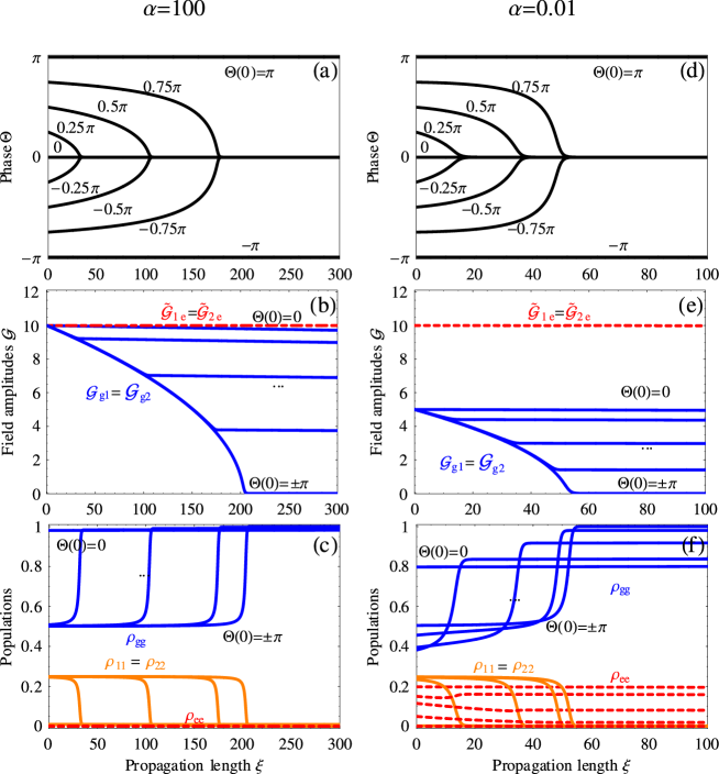
Figure 8: (color online) Propagation of relative phase (a), field amplitudes (b), and populations of the atomic levels (c), for various input phases $\Theta(0)=0,\pm\pi/4,\pm\pi/2,\pm 3\pi/4,\pi$. The upper fields are saturated at least as deeply as the lower fields. Curves (a-c) are obtained for input parameters $\alpha=100$, and $\mathcal{G}_{g}=\mathcal{\tilde{G}}_{e}=10$. Curves (d-f) have input parameters $\alpha=0.01$, $\mathcal{G}_{g}=5$ and $\mathcal{\tilde{G}}_{e}=10$. During propagation the phase tends to $\Theta=0$. Once this phase is reached, the rate of energy dissipation along the medium changes abruptly to a significantly lower level. In the case(d-f) this change is accompanied by the establishing of population inversion on the transition $|{1}\rangle,|{2}\rangle\to|{e}\rangle$, see (f), due to the formation of EIT-coherences.

Having identified and investigated two special values of the input phase, we now address the question, how the phase evolves starting from a generic input value, and correspondingly, how light propagates and is dissipated along the medium. We restrict to the configuration with initially equal lower field amplitudes and equal upper field amplitudes (33) and (34), and vary the input phase $\Theta(0)=\pi/2$ in steps of $\pi/4$.

Figures 8 and 9 display the amplitude and the relative phase of the propagating fields for different values of the excited state decay rate: $\alpha=100$ and $\alpha=0.01$. Although the lower field amplitudes are clearly damped for all values of $\alpha$, the mechanism of radiation dissipation depends on $\alpha$ and on the initial strengths of the field amplitudes. This can be associated with a particular evolution of the phase along the medium, which in the cases displayed in Fig. 8 reaches the stable value $\Theta=0$, and in the cases displayed in Fig. 9 tends first to the value $\pi$ before eventually reaching $\Theta=0$. The choice between these behaviors depends on the input amplitudes of the fields. We now discuss these two behaviors in detail.

In Fig. 8 all atomic transitions are driven at saturation, and the saturation of the upper transitions is larger or equal to that of the lower transitions. We observe that the relative phase of the fields tends to the zero value. Before this value is reached, radiation is damped at a fast rate. Once $\Theta=0$, the rate of damping of the lower field amplitudes changes abruptly to a lower value. This sudden change occurs at a propagation length determined by the typical absorption length of the fast decaying transition. The system simulates a V-configuration, thereby switching to an EIT-like response. A similar kind of behavior is also observed in a medium of the Double-$\Lambda$ atoms where EIT-coherences are established between the two stable states Korsunsky99 . In the $\diamondsuit$ configuration the coherences and interferences are transient Windholz96 . For a slower decay of the excited state, however, the system can also switch to a $\Xi$-dynamics and exhibit a transient coherence between ground and excited states. A manifestation of this phenomenon is population inversion between the excited and the intermediate states along the medium in Fig. 8(f).

In Fig. 9 the lower transitions are driven well above saturation, and the corresponding saturation parameter is larger than the saturation parameter of the upper fields. Here, during a transient regime the phase slowly tends to $\Theta=\pi$. Nonetheless, the tendency of the medium for long propagation lengths is to eventually decouple upper fields and atoms, i.e. to switch to a V-dynamics. The onset of this dynamics depends critically on the value of $\mathcal{G}_{g}$, which must well saturate the lower transitions with respect to $\mathcal{G}_{e}$ in order to populate the intermediate states on a time scale shorter than their decay rate, but long enough for incoherent decay of the upper state to take place. This behavior is in agreement with Sec. III.4, showing that when the lower transitions are driven well above saturation the value $\Theta=\pi$ is the only stable phase under amplitude and phase fluctuations.

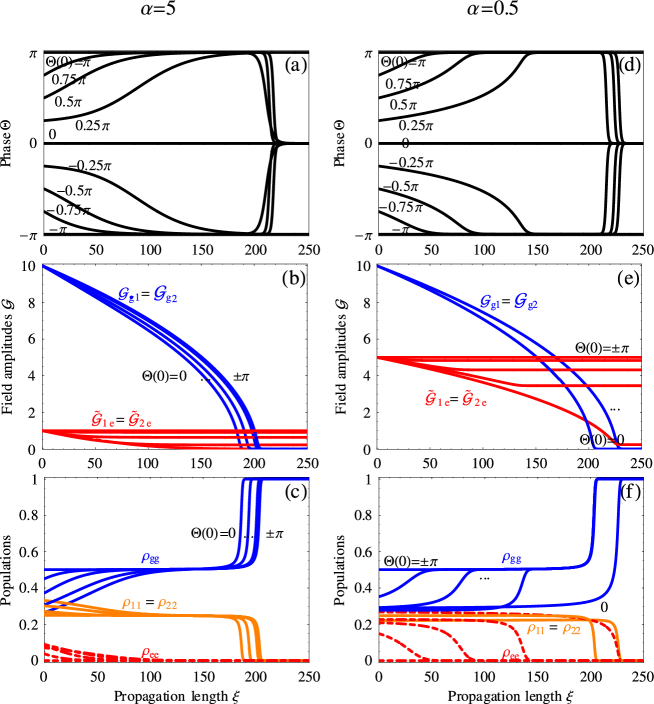
Figure 9: (color online) Propagation of relative phase (a), field amplitudes (b), and populations of the atomic levels (c), for various input phases $\Theta(0)=0,\pm\pi/4,\pm\pi/2,\pm 3\pi/4,\pi$. Curves (a-c) are obtained for input parameters $\alpha=5$, and $\mathcal{G}_{g}=10$, $\mathcal{\tilde{G}}_{e}=1$, and curves (d-f) for $\alpha=0.5$ and the same initial amplitudes. Here, the lower transitions are driven well above saturation and during a transient regime the phase tends to the value $\pi$, while the upper fields decouple. The transition to the value $\Theta=0$ at large values of $\xi$ is an artifact, since for these lengths the lower fields are very weak and the atoms are essentially in the ground state.

III.6 Four-wave mixing

So far, we have considered input fields with equal lower and upper field amplitudes. We now discuss propagation when one field is initially very weak while the other three transitions are driven at or above saturation, and study how the dynamics of energy redistribution among the fields depends on the input parameters and on the stability of the excited state.

Figures 10 and 11 display the field propagation when the upper field amplitude $\mathcal{G}_{e2}$ is very small and the phase is initially set to the value $\Theta(0)=\pi/2$. In both figures we have assumed the excited state to decay slower than the intermediate states, but one may also observe amplification of the weak field under different conditions. In Fig. 10 the three input fields drive the respective transitions well above saturation. Here, amplification of the weak field is accompanied by the asymptotic approaching of the phase to $\Theta=\pi$. The field $\mathcal{G}_{e2}$ is amplified until the upper state is depleted because of interference between the upper fields. From this point further the phase $\Theta=\pi$ is stable and the lower fields dissipate, until they drop below saturation. The jump of the phase to the value 0 is an artifact due to all atoms being in the ground state.

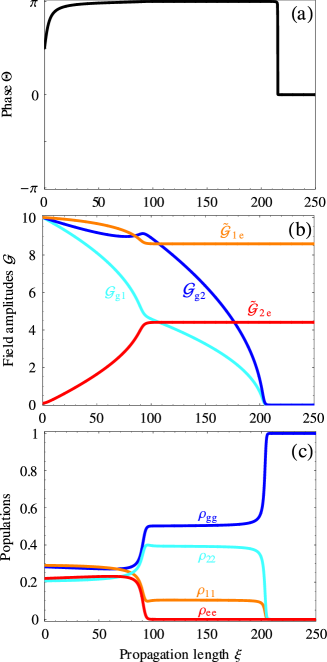
Figure 10: (color online) (a) Propagation of relative phase (a), field amplitudes (b), and atomic populations (c) for input parameters $\Theta=\pi/2$, $\alpha=0.1$, $\mathcal{G}_{g1}=\mathcal{G}_{g2}=\mathcal{G}_{1e}=10$, and $\mathcal{G}_{2e}=0.1$. Energy is exchanged between fields $\mathcal{G}_{2e}$ and $\mathcal{G}_{g1}$ and also between $\mathcal{G}_{1e}$ and $\mathcal{G}_{g2}$ until the excited state decouples and the upper fields propagate freely. The jump of the phase to the value 0 is an artifact due to all atoms being in the ground state.

In Fig. 11 the three input fields $\mathcal{G}_{1g},\mathcal{G}_{2g}$ and $\mathcal{G}_{e1}$ are just saturating the respective transitions. Here, amplification of the field $\mathcal{G}_{e2}$ is accompanied by a transient stabilization of the phase at $\Theta=\pi$. This is accompanied by a fast decrease of the lower field amplitude $\mathcal{G}_{g2}$, until, when $\mathcal{G}_{g2}$ vanishes, the phase falls to $\Theta=0$. After this point the behavior changes and $\mathcal{G}_{g2}$ first increases slightly and then decays slowly as a function of $\xi$ in a way similar to $\mathcal{G}_{g1}$, while the upper field amplitudes remain constant. The final configuration supports a coherence between the excited and the ground state, and indeed for $\Theta=0$ and this value of $\alpha$ the dynamics can be mapped to a $\Xi$-level scheme. In particular, due to destructive interference, the fields are only weakly coupled to the transitions and the medium is semitransparent. This is also supported by Fig. 11(c) where one sees that the population is redistributed between the ground and the excited state while the intermediate states are depleted. In this regime the medium is characterized by population inversion between the excited and the intermediate states.

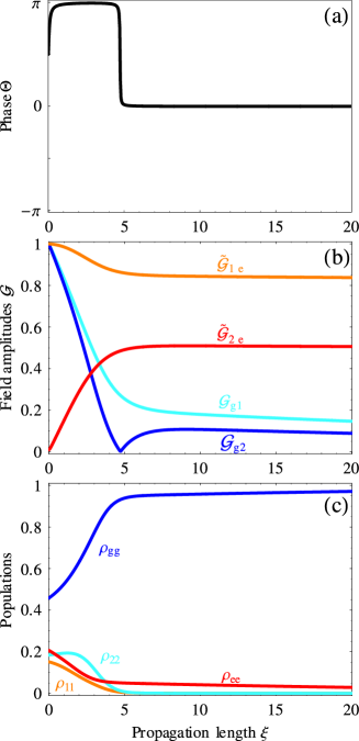
Figure 11: (color online) (a) Propagation of relative phase (a), field amplitudes (b), and atomic populations (c) for input parameters $\Theta=\pi/2$, $\alpha=0.01$, $\mathcal{G}_{g1}=\mathcal{G}_{g2}=\mathcal{\tilde{G}}_{1e}=1$, and $\mathcal{\tilde{G}}_{2e}=0.01$. The amplitude $\mathcal{\tilde{G}}_{2e}$ while the phase approaches $\Theta=\pi$. At the same time $\mathcal{\tilde{G}}_{1e}$ gradually vanishes at which point the phase changes to $\Theta=0$ and the fields propagate almost undamped.

IV Discussion and conclusions

We have investigated numerically light propagation in a medium of atoms whose electronic levels are resonantly driven by lasers in a $\diamondsuit$ configuration. Propagation is critically affected by the initial parameters of the input fields and shows the tendency to reach configurations which minimize dissipation. An important role is played by the relative phase $\Theta$ between the fields. It exhibits two fixed points, $\Theta=0$ and $\Theta=\pi$, whose stability during propagation depends on the field amplitudes and on the ratio $\alpha$ between the rates of dissipation of excited and intermediate states. A generic input phase evolves, in general, to one of these values, again depending on the input amplitudes and $\alpha$.

These two metastable phase values are associated with two different types of atomic coherences. The response of the medium, corresponding to the phase $\Theta=0$, is characterized by the formation of atomic coherences typical of EIT-media. Similar behaviors have been observed for instance in VandenHeuwell ; Windholz96 and are analogous to the response predicted for light propagation in double-$\Lambda$ media Korsunsky99 .

The response of the medium for the phase $\Theta=\pi$ is supported by a different type of interference which leads to a depletion of the upper state and to a complete decoupling of the upper fields from the atom. For this value of the phase, the medium acts like a $V$-level configuration. We note that this value of the phase appears to be the preferred value for the $\diamondsuit$ medium if the lower transitions are driven well above saturation. This behavior is novel to our knowledge and it is reminiscent of the phenomenon of suppression of spontaneous emission observed in four-wave mixing studies in atomic gases Boyd .

In general, the system exhibits a rich dynamics and several novel features due to atomic coherence which offer new perspectives in control techniques in quantum electronics. These could be studied in atomic gases where the ground state has no hyperfine multiplet, like e.g. alkali-earth isotopes which are currently investigated for atomic clocks AlkaliEarth .

In the future we will extend our analysis to the case in which the transitions are not resonantly driven and we will address the asymptotic behavior of the system following the lines of recent works Korsunsky02 ; Johnsson .

Appendix A Macroscopic Polarization in the semiclassical limit for the atomic motion

We consider the dynamics of the density matrix $\varrho$ of the atomic internal and external degrees of freedom, where the center-of-mass degrees of freedom are treated as classical variables. Hence, the position ${\bf x}$ and momentum ${\bf p}$ are parameters, distributed according the function $w({\bf x},{\bf p})$ which we assume to be stationary, with $\int{\rm d}{\bf x}{\rm d}{\bf p}w({\bf x},{\bf p})=N$ and $N$ is the number of atoms. The spatial density of atoms $n({\bf x})$ is found from $w({\bf x},{\bf p})$ according to $\int{\rm d}{\bf p}w({\bf x},{\bf p})=n({\bf x})$. In this work we assume uniform density, namely

$$n({\bf x})=n$$

with $n$ constant. The master equation for the density matrix $\varrho$, at the point $({\bf x},{\bf p})$ in phase space has the form

$$\dot{\varrho}=\frac{1}{{\rm i}\hbar}\left[H({\bf x},{\bf p};t),\varrho\right]+\mathcal{L}\varrho$$ (44)

where the Hamiltonian $H({\bf x},{\bf p};t)$ contains the coherent dynamics of the atoms driven by the classical field,

$$H({\bf x},{\bf p};t)=\frac{{\bf p}^{2}}{2M}+H(z,t)$$ (45)

and $H(z,t)$ is defined in Eq. (II.2). The Liouvillian $\mathcal{L}$ in Eq. (16) describes the relaxation processes, which we consider here to be purely radiative. The corresponding macroscopic polarization has the form

$${\bf P}({\bf x},t)=\int{\rm d}{\bf p}w({\bf x},{\bf p})\operatorname{Tr}\{{\bf\hat{d}}\varrho({\bf x},{\bf p})\}$$ (46)

Assuming that the atomic gas has been Doppler cooled, so that line broadening is homogeneous, the kinetic energy can be neglected in evaluating the atomic response to the light. By integrating over ${\bf p}$ and $x,y$ we hence obtain Eq. (14), whereby $\sigma(z)=\int{\rm d}{\bf p}{\rm d}x{\rm d}yw({\bf x},{\bf p})\sigma({\bf x},{\bf p})$, and polarization as in Eq. (2).

Appendix B Optical Bloch Equations in the phase- reference frame

We consider Master Eq. (18) in the reference frame of the phase. With the notation $\tilde{\rho}_{e2}=\rho_{e2}\;\text{exp}\left(-i\Theta\right)$, the corresponding optical Bloch equations are given by

$$\dot{\rho}_{ee} = i\frac{\Omega_{1e}}{2}(\rho_{1e}-\rho_{e1})+i\frac{\Omega_{2e}}{2}(\tilde{\rho}_{2e}$$

$$-\tilde{\rho}_{e2})-\gamma_{e}\rho_{ee}$$

$$\dot{\rho}_{11} = -i\frac{\Omega_{1e}}{2}(\rho_{1e}-\rho_{e1})+i\frac{\Omega_{1g}}{2}(\rho_{g1}-\rho_{1g})$$ (48)

$$+\frac{\gamma_{e}}{2}\rho_{ee}-\gamma_{1g}\rho_{11}$$

$$\dot{\rho}_{22} = -i\frac{\Omega_{2e}}{2}(\tilde{\rho}_{2e}-\tilde{\rho}_{e2})+i\frac{\Omega_{2g}}{2}(\rho_{g2}-\rho_{2g})$$ (49)

$$+\frac{\gamma_{e}}{2}\rho_{ee}-\gamma_{2g}\rho_{22}$$

$$\dot{\rho}_{e1} = \left(i\left(\Delta_{1}-\Delta_{e}\right)-\frac{\gamma_{e}+\gamma_{1g}}{2}\right)\rho_{e1}$$

$$+i\frac{\Omega_{1e}}{2}(\rho_{11}-\rho_{ee})+i\frac{\Omega_{2e}}{2}e^{i\Theta}\rho_{21}-i\frac{\Omega_{1g}}{2}\rho_{eg}$$

$$\dot{\tilde{\rho}}_{e2} = \left(i\left(\Delta_{2}-\Delta_{e}\right)-\frac{\gamma_{e}+\gamma_{2g}}{2}\right)\tilde{\rho}_{e2}$$

$$+i\frac{\Omega_{2e}}{2}(\rho_{22}-\rho_{ee})+i\frac{\Omega_{1e}}{2}e^{-i\Theta}\rho_{12}-i\frac{\Omega_{2g}}{2}e^{-i\Theta}\rho_{eg}$$

$$\dot{\rho}_{1g} = -\left(i\Delta_{1}+\frac{\gamma_{1g}}{2}\right)\rho_{1g}+i\frac{\Omega_{1e}}{2}\rho_{eg}$$

$$-i\frac{\Omega_{2g}}{2}\rho_{12}+i\frac{\Omega_{1g}}{2}(\rho_{gg}-\rho_{11})$$

$$\dot{\rho}_{2g} = -\left(i\Delta_{2}+\frac{\gamma_{2g}}{2}\right)\rho_{2g}+i\frac{\Omega_{2e}}{2}e^{-i\Theta}\rho_{eg}$$

$$-i\frac{\Omega_{1g}}{2}\rho_{21}+i\frac{\Omega_{2g}}{2}(\rho_{gg}-\rho_{22})$$

$$\dot{\rho}_{12} = \left(i\left(\Delta_{2}-\Delta_{1}\right)-\frac{\gamma_{1g}+\gamma_{2g}}{2}\right)\rho_{12}+i\frac{\Omega_{1e}}{2}e^{i\Theta}\tilde{\rho}_{e2}$$ (54)

$$+i\frac{\Omega_{1g}}{2}\rho_{g2}-i\frac{\Omega_{2g}}{2}\rho_{1g}-i\frac{\Omega_{2e}}{2}e^{i\Theta}\rho_{1e}$$

$$\dot{\rho}_{eg} = -\left(i\Delta_{e}+\frac{\gamma_{e}}{2}\right)\rho_{eg}+i\frac{\Omega_{1e}}{2}\rho_{1g}$$ (55)

$$+i\frac{\Omega_{2e}}{2}e^{i\Theta}\rho_{2g}-i\frac{\Omega_{1g}}{2}\rho_{e1}-i\frac{\Omega_{2g}}{2}e^{i\Theta}\tilde{\rho}_{e2}.$$

where $\rho_{ij}=\rho_{ji}^{*}$, $\rho_{gg}=1-\rho_{ee}-\rho_{11}-\rho_{22}$, and we have taken $\gamma_{e1}=\gamma_{e2}=\gamma_{e}/2$.

References

- (1) S.E. Harris, Phys. Today 50, 36 (1997); E. Arimondo, Prog. Opt. 35, 259 (1996).
- (2) D.A. Braje, V. Balic, S. Goda, G.Y. Yin, and S.E. Harris, Phys. Rev. Lett. 93, 183601 (2004).
- (3) V. Balic, D.A. Braje, P. Kolchin, G.Y. Yin, and S.E. Harris, Phys. Rev. Lett. 94, 183601 (2005).
- (4) M.D. Eisaman, L. Childress, A. André, F. Massou, A.S. Zibrov, and M.D. Lukin, Phys. Rev. Lett. 93, 233602 (2004).
- (5) A. Nottelmann, C. Peters, and W. Lange, Phys. Rev. Lett. 70, 1783 (1993)
- (6) C. Peters and W. Lange, App. Phys. B 62, 221 (1996)
- (7) J. Guo, P. R. Berman, B. Dubetsky, and G. Grynberg, Phys. Rev. A 46, 1426 (1992).
- (8) M. Vengalattore and M. Prentiss, Phys. Rev. Lett. 95, 243601 (2005)
- (9) S.J. Buckle, S.M. Barnett, P.L. Knight, M.A. Lauder, and D.T. Pegg, Optica Acta 33, 1129 (1986).
- (10) D.V. Kosachiov, B.G. Matisov, and Y.V. Rozhdestvensky, J. Phys. B: At. Mol. Opt. Phys. 25, 2473 (1992).
- (11) E.A. Korsunsky and D.V. Kosachiov, Phys. Rev. A 60, 4996 (1999).
- (12) G. Morigi, S. Franke-Arnold, G.-L. Oppo, Phys. Rev. A 66, 053409 (2002)
- (13) M.D. Lukin, P.R. Hemmer, and M.O. Scully, Adv. At. Mol. Opt. Phys. 42, 347 (2000).
- (14) H. Shpaisman, A.D. Wilson-Gordon, and H. Friedmann, Phys. Rev. A 70, 063814 (2004); Phys. Rev. A 71, 043812 (2005).
- (15) W.E. van der Veer, R.J.J. van Diest, A. Donszelmann, and H.B. van Linden van den Heuvell, Phys. Rev. Lett. 70, 3243 (1993).
- (16) W. Maichen, F. Renzoni, I. Mazets, E. Korsunsky, and L. Windholz, Phys. Rev. A 53, 3444 (1996).
- (17) A.J. Merriam, S.J. Sharpe, M. Shverdin, D. Manuszak, G.Y. Yin, and S.E. Harris, Phys. Rev. Lett. 84, 5308 (2000).
- (18) E.A. Korsunsky, N. Leinfellner, A. Huss, S. Baluschev, and L. Windholz, Phys. Rev. A 59, 2302 (1999).
- (19) A.F. Huss, R. Lammegger, C. Neureiter, E.A. Korsunsky, and L. Windholz, Phys. Rev. Lett. 93, 223601 (2004).
- (20) V.S. Malinovsky and I. R. Sola, Phys. Rev. Lett. 93, 190502 (2004); Phys. Rev. A 70, 042304 (2004); Phys. Rev. A 70, 042305 (2004).
- (21) R. Santra, E. Arimondo, T. Ido, C.H. Greene, and J. Ye, Phys. Rev. Lett. 94, 173002 (2005); T. Ido, T.H. Loftus, M.M. Boyd, A.D. Ludlow, K.W. Holman, and J. Ye, Phys. Rev. Lett. 94, 153001 (2005).
- (22) M.O. Scully and M.S. Zubairy, Quantum Optics (Cambridge University Press, Cambridge, 1997).
- (23) L. Allen and J.H. Eberly, Optical Resonance and Two-level atom (Wiley, New York, 1975).
- (24) For this behavior becomes evident after rescaling the field amplitudes, Eq. (9), with the linewidth and then letting .
- (25) R. M. Whitley and C. R. Stroud, Jr., Phys. Rev. A 14, 1498 (1976).
- (26) M.S. Malcuit, D.J. Gauthier, and R.W. Boyd, Phys. Rev. Lett. 55, 1086 (1985); R.W. Boyd, M.S. Malcuit, D.J. Gauthier, and K. Rzaewski, Phys. Rev. A 35, 1648 (1987).
- (27) E.A. Korsunsky and M. Fleischhauer, Phys. Rev. A 66, 033808 (2002).
- (28) M.T. Johnsson and M. Fleischhauer, Phys. Rev. A 66, 043808 (2002).