Energy flow in a hadronic cascade: Application to hadron calorimetry

Abstract

The hadronic cascade description developed in an earlier paper is extended to the response of an idealized fine-sampling hadron calorimeter. Calorimeter response is largely determined by the transfer of energy $E_{\pi^{0}}$ from the hadronic to the electromagnetic sector via $\pi^{0}$ production. Fluctuations in this quantity produce the “constant term” in hadron calorimeter resolution. The increase of its fractional mean, $f_{\pi^{0}}^{0}=\left\langle E_{\pi^{0}}\right\rangle/E$, with increasing incident energy $E$ causes the energy dependence of the $\pi/e$ ratio in a noncompensating calorimeter. The mean hadronic energy fraction, $f^{0}_{h}=1-f_{\pi^{0}}^{0}$, was shown to scale very nearly as a power law in $E$: $f^{0}_{h}=(E/E_{0})^{m-1}$, where $E_{0}\approx 1$ GeV for pions, and $m\approx 0.83$. It follows that $\pi/e=1-(1-h/e)(E/E_{0})^{m-1}$, where electromagnetic and hadronic energy deposits are detected with efficiencies $e$ and $h$, respectively. If the mean fraction of $f^{0}_{h}$ which is deposited as nuclear gamma rays is $f^{0}_{\gamma}$, then the expression becomes $\pi/e=1-(1-h^{\prime}/e)(1-f^{0}_{\gamma})(E/E_{0})^{m-1}$. Fluctuations in these quantities, along with sampling fluctuations, are incorporated to give an overall understanding of resolution, which is different from the usual treatments in interesting ways. The conceptual framework is also extended to the response to jets and the difference between $\pi$ and $p$ response.

1 Introduction

In Paper I[1] we developed a conceptual basis for understanding the division between hadronic and electromagnetic (actually $\pi^{0}$) energy deposition in a contained hadronic cascade. The model “calorimeter” was a very large iron or lead cylinder, with no energy leakage except via muons, neutrinos, and front-surface albedo losses. Extensive Monte Carlo simulations gave results in good agreement with test-beam measurements. The relevant conclusions of the paper were that:

1. All significant hadronic energy deposition is by low-energy particles($\mathrel{\hbox to0.0pt{\raise 2.20013pt\hbox{$<$}\hss}{\lower 2.20013pt\hbox{$\sim$}}}1$ GeV), whose energy and species distribution in a given medium is independent of the energy or species of the incident hadron. (Hadronic energy was defined as all energy not carried away by $\pi^{0}$ decay photons.) The existence of this “universal low-energy hadron (and nuclear gamma ray) spectrum” makes it possible to define an energy-independent efficiency $h$ for the conversion of this energy into a visible signal in a fine-sampling calorimeter.

2. In each high-energy collision of the hadronic cascade, a significant fraction (typically 1/4) of the energy is lost from further hadronic activity via $\pi^{0}$ production. A sequence of high-energy hadronic collisions bleeds off a larger and larger fraction of the energy as the incident energy $E$ increases. The net fraction transferred to the $\pi^{0}$ sector in a given cascade is $f_{\pi^{0}}$, and the mean $\pi^{0}$ fraction is $f_{\pi^{0}}^{0}$. This one-way flow is illustrated in Fig. 1.

   

   
   

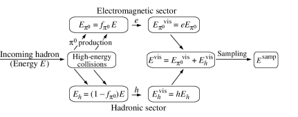
   Figure 1: Energy flow in a hadronic cascade. A fraction $f_{\pi^{0}}$ (with energy-dependent mean $f_{\pi^{0}}^{0}$) is transferred to the electromagnetic sector through $\pi^{0}$ production in repeated hadronic inelastic collisions. The $\pi^{0}$ and hadronic energy deposits after the division are separately stochastic, and so must be treated as parallel statistical processes. Each produces a visible signal, whose sum $E^{\rm vis}$ is sampled.

3. In particular, the mean fraction of the energy $f^{0}_{h}=1-f^{0}_{\pi^{0}}$ in the hadronic sector scales very nearly as a power of the incident energy,

   $$f^{0}_{h}(E)=(E/E_{0})^{m-1}\ ,$$ (1)

   where $m\approx 0.83$ (with some mild absorber $Z$ dependence) and $E_{0}\approx 1$ GeV for pions and $\approx 2.6$ GeV for protons (again, with some $Z$ dependence). Physically, $m$ is related to the mean number of secondaries and the mean energy fraction going into $\pi^{0}$’s in any given collision in the cascade, and $E_{0}$ is the energy at which multiple pion production becomes significant. Both must be determined by experiment for a given calorimeter.

4. It was predicted that a calorimeter would have a different response to a proton than to a pion.

The observations pertain equally well to a homogeneous or fine-sampling calorimeter, and have significant implications for its response and resolution. “Fine-sampling” means that absorber and sensor elements are thin compared to both the em radiation length and the neutron interaction length. It has the same structure throughout: no separate front em compartment or rear catcher. It can be an inorganic crystal calorimeter, a uranium/liquid argon calorimeter, or a lead/scintillator-fiber calorimeter.

The power-law approximation given in Eq. (1) is just that, for reasons discussed in Paper I. It seems to work well over the energy range of available test-beam data, about 10 GeV to 375 GeV, and it has the required asymptotic properties: It is everywhere positive, and $f^{0}_{h}\to 0$ ($\pi/e\to 1$) as $E\to\infty$. The physical assumptions it is based upon become less dependable at very high energies and are not valid at energies below the threshold for multiple pion production.

As far as possible, results in this paper are obtained without recourse to the power-law approximation for $f^{0}_{h}$, in order to obtain more general results than those relying on this more approximate form.

Most of the results reported in this paper can be found in the Proceedings of various conferences and workshops[2, 4, 5, 6, 7, 8, 9]. The Monte Carlo results used in these papers are often based on now-superseded versions of hadronic cascade simulation codes[10], the oldest being FLUKA86. In particular, nuclear gamma rays were not included, so that the em deposit is exclusively via $\pi^{0}$ production. Since these versions many improvements in the codes have been made, e.g., improvements in FLUKA by Ferrari and Sala[11], especially in the nuclear physics modeling. The failings of the old code are apparent in Fig. 2(b), for example, where the points fall below the 45^∘ line because of unscored hadronic energy. A large fraction of the unscored energy is evidently that of nuclear gamma rays. On the other hand, ${\pi^{0}}$ energy deposition was very well described[12] and can be trusted. In Paper I we reported simulations with MARS10, HETC, and FLUKA, which, though based on different high-energy interaction models, were in excellent agreement. Since in this paper I depend only upon the high-energy division between the $\pi^{0}$ and hadronic sectors, calculations based on the older code have not been repeated.

In Sec. 3, I distinguish between em energy deposit by $\pi^{0}$ decay photons and by nuclear de-excitation gamma rays. A fraction $f_{{\pi^{0}}}$ of the energy is deposited via ${\pi^{0}}$ decay, and a fraction $f_{h}f_{\gamma}$ by nuclear gamma rays within the acceptance gate, where $f_{h}=1-f_{\pi^{0}}$. The total em deposit is $E_{\pi^{0}}+E_{\gamma}=E(f_{\pi^{0}}+f_{h}f_{\gamma})$.

Recent developments are incorporated, some of which were predicted or discussed in Paper I. These include Cherenkov readout[13], which is sensitive only to em ($\pi^{0}$ and nuclear gamma) energy deposition, and observation of the $\pi/p$ response difference[14].

Central to the paper is the discussion of resolution, where conditional probability distribution functions (p.d.f.’s) are combined to account for parallel, independent stochastic processes.

Hadron calorimetry is a well-traveled road, explored in hundreds, if not thousands, of papers over several decades. The object here is to present a broad-brush treatment of hadronic cascades in a simplified generic calorimeter, in hopes that a somewhat nonstandard approach can contribute to our physical understanding of a real calorimeter. Real calorimeters, with front em compartments, rear catchers, leakage, crack corrections, jet finding algorithms, and a myriad of other features, are described in dozens of test-beam study results, as well as in published studies of compensation, the role of neutrons, and other matters. These are discussed in detail in Wigmans’ book[3] and review[15], the review by Leroy and Rancoita[16], and in their many citations. None of these practical problems are discussed here.

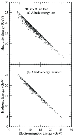
Figure 2: Calculated energy deposit distributions for 30 GeV negative pions incident on a lead “calorimeter.” In case (a) backscattered energy is lost; in (b) it is retained.

2 Albedo and $f_{\pi^{0}}$

The $\pi^{0}$ fraction $f_{\pi^{0}}=E_{\pi^{0}}/E$ increases with energy, but at any given energy it is subject to large fluctuations. FLUKA simulations of the $\pi^{0}$/hadronic energy division are shown in Fig. 2. The model absorber consisted of a large lead cylinder (50 cm radius, 250 cm long) in which the first 25 cm (about 1.5 interaction lengths) was treated as a separate region. In Fig 2(a) no distinction is made between the regions, while in  2(b) interaction of the incident pion was not permitted in the front section, but energy deposited there is included. It acted as a catcher for back-scattered interaction debris. The distribution about the ideal $E_{h}=1-E_{\pi^{0}}$ shows less scatter in 2(b) because front-face, or albedo, losses are included. Most albedo loss comes from backward or backscattered products of the first collision; when the first interaction occurs deep in the detector there is essentially no albedo loss. Runs at 50 GeV with and without an “albedo catcher” show an average difference in deposited energy is 0.43 GeV, or 0.8%. Out of 1000 cascades 50% lost less than 0.2 GeV, and 3.4% lost more than 2 GeV. In the simulations the amount of lost albedo energy rises only slowly with increasing incident energy, as might be expected. While these losses are not totally negligible, I omit them from resolution considerations in Sec, 7 because (a) the distribution is sharply peaked at near-zero loss, and (b) the losses are small, particularly at higher energies.

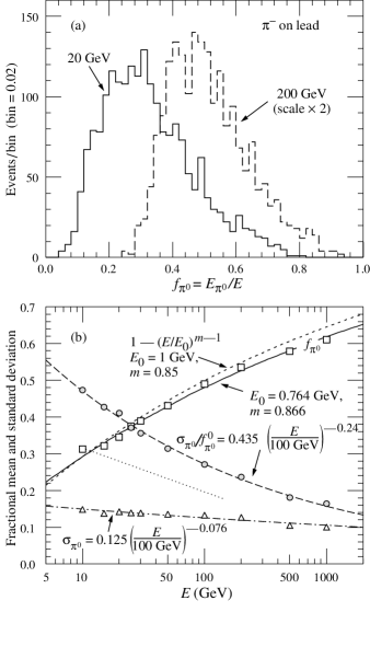
Figure 3: FLUKA simulations for negative pions incident on a lead “calorimeter.” (a) Distribution of the ${\pi^{0}}$ energy deposit for 20 and 200 GeV incident pions, and (b) energy dependence of the mean ($\left\langle f_{\pi^{0}}\right\rangle=f^{0}_{\pi^{0}}$), standard deviation ($\sigma_{\pi^{0}}$) of the $f_{\pi^{0}}$ distribution, and standard deviation relative to the mean ($\sigma_{\pi^{0}}/f_{0}$). The dotted line is discussed in the text.

For reasons discussed in the introduction, the points shown in Fig. 2 scatter below the 45^∘ line because older versions of FLUKA did not account for all of the hadronic energy deposit, even in the absence of albedo losses. Presumably most of this downward scatter (about 15% in the worst case) is the result of the program’s failure to tally nuclear gamma rays, most of which come from de-excitation following slow neutron capture by nuclei. According to Ferrari and Sala[17], these might account for nearly 10% (Fe) or 20% (Pb) of the $\pi^{0}+\gamma$ fraction, or 5%–10% of the total energy deposit. These contributions scale with the hadronic fraction, not the $\pi^{0}$ fraction. Given that the hadronic fraction is underestimated by this fraction in this simulation, it is better to take the hadronic fraction as

$$f_{h}\equiv 1-f_{\pi^{0}},\ {\rm{or}}\ E_{h}\equiv E-E_{\pi^{0}}\ .$$ (2)

As the number of Monte Carlo events in the sample increases, the $(E_{h},E_{\pi^{0}})$ distribution projected onto the $E_{\pi^{0}}$ axis approaches the marginal distribution $\Pi(f_{\pi^{0}})$, the p.d.f  of the $\pi^{0}$ energy fraction. Two (unnormalized) FLUKA-generated examples of $f_{\pi^{0}}\equiv E_{\pi^{0}}/E$ distributions are shown in Fig. 3(a). The mean and standard deviations are shown in Fig. 3(b).

The fractional mean $f_{\pi^{0}}^{0}$ moves slowly to the right with increasing energy, and can be represented by $f_{\pi^{0}}^{0}=1-(E/E_{0})^{m-1}$. As it does so, the rms width of the distribution decreases only slowly (presumably because of increasing ${\pi^{0}}$ multiplicity), and is well-represented by

$$\sigma_{\pi^{0}}=12.5\%\times(E/100\,\rm{GeV})^{-0.076}\ .$$ (3)

There is no physical basis for this functional form, except that it remains positive as $E\to\infty$. As the incident energy becomes very large, the distribution “crowds” the right limit, and the variance should approach zero. The fits to real data (Fig. 14 and Tbl. LABEL:tab:fitparameters) yield somewhat different values for the multiplier and exponent, which in any case should vary from case to case.

Alternatively, one might have chosen to express the width as a fraction of the mean rather than as a fraction of the total incident energy, or as $\sigma_{\pi^{0}}/f_{\pi^{0}}^{0}$ rather than $\sigma_{\pi^{0}}$. A power-law fit to the Monte Carlo data in this form is indicated by the dashed line in Fig. 3(b). The strong energy dependence just reflects the energy dependence of $f_{\pi^{0}}^{0}$, and the mildness of the energy dependence of $\sigma_{\pi^{0}}$ is obscured.

The dotted line in Fig. 3(b) is a fit by Acosta et al. to SPACAL data for $\sigma_{\rm rms}(f_{1})/f_{1}$ in the range 10–150 GeV, where “1” refers to the central tower[18]. The authors show that the $f_{1}$ distribution is a good representation of the $f_{\pi^{0}}$ distribution. The fit is given as $0.435-0.052\ln(E)$. SPACAL was a lead/scintillator fiber calorimeter, while our model is a solid lead cylinder. The test beam events contained contributions from nuclear gamma rays. Even so, the difference between the dotted line and the FLUKA-simulation dashed line is difficult to understand.

The dimensionless “coefficient of skewness,” $\gamma_{1}=\mu_{3}/\sigma_{\pi^{0}}^{3}$ (where $\mu_{3}$ is the third moment about the mean), is constant to within the Monte Carlo statistics with a value near 0.6. There are no significant higher moments within the sensitivity of the simulations. One might expect to see the skewness change sign; the tail should move from the right to the left side of the most probable value at very high energies. This transition has not yet been observed.

It is instructive to examine a continuous distribution with similar properties: the Beta distribution $f(x;p,q)=x^{q-1}(1-x)^{s-1}/B(p,q)$, where the normalizing constant $B(p,q)$ is the Beta function[19]. It may be thought of as “a continuous version of the binomial distribution:” It is defined only for $0\leq x\leq 1$, is zero at both limits, and the peak position, variance, and other properties depend on $p$ and $q$. For $p>2$ and $q>2$ it has zero derivative at both limits. If the mean is less than 0.5 the distribution is skewed to the right, as is the case for $\Pi(f_{\pi^{0}})$; for larger means the distribution is skewed to the left. The skewness of $\Pi(f_{\pi^{0}})$ remains positive for means much greater than 0.5, but, as explained above, might be expected to change sign as the mean approaches unity.

Different or better cascade simulations would be expected to produce distributions with somewhat different shapes and different moments. What is of consequence here is that a function $\Pi(E_{\pi^{0}})$ exists which describes the energy distribution of the $\pi^{0}$’s for a given primary energy $E$; no significant conclusions in this paper depend upon the details.

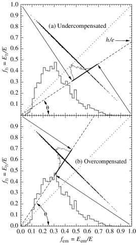
Figure 4: The projection of “events” onto the diagonal line at $\theta=\tan^{-1}(h/e)$ gives the energy distribution for a calorimeter in the absence of any other fluctuations. Events must fall along the thick solid segments. One can imagine the projection as $\theta$ increases from 0^∘ ($h/e=0$, large dotted histogram through the undercompensated case shown in (a)) to 45^∘ ($h/e=1$, full compensation) where it approaches a $\delta$-function. For $\theta>45^{\circ}$ ($h/e>1$, shown in (b)), the calorimeter is overcompensated, and the skewness changes sign.

The contribution of $\Pi(f_{\pi^{0}})$ to the calorimeter resolution can be understood by a geometrical construction. Figure 4 shows the same MC “events” as Fig. 2(b), but with the lost hadronic energy restored as per Eq. (2) (except for some vertical scatter retained for clarity). The observed energy distribution in the absence of sampling fluctuations is the projection of this distribution onto a diagonal line at $\theta=\tan^{-1}(h/e)$. The limits of the projected distribution ($f_{\pi^{0}}=0$ and $f_{\pi^{0}}=1$) are shown by the arrows. All of the events thus project onto the solid segment of the line, with length $|\cos\theta-\sin\theta|=(1-h/e)\cos\theta$. The sampled $\Pi(f_{\pi^{0}})$ distribution in Fig. 3(b) is replotted as the histogram along the $f_{\pi^{0}}$ axis. A point at $f_{\pi^{0}}=1$ projects to the end of the solid segment, so the energy scale along this axis is foreshortened by $\cos\theta$. The length of the solid line segment, rescale by $1/\cos\theta$, is $(1-h/e)$. The fractional standard deviation of $\Pi(f_{\pi^{0}})$, $\sigma_{\pi^{0}}$, also scales as $(1-h/e)$. It thus contributes $(1-h/e)\sigma_{\pi^{0}}$ (in quadrature) to the calorimeter resolution.

For $h/e=1$, $\theta=45^{\circ}$ and the distribution becomes a $\delta$-function. For $h/e>1$ (overcompensation) the distribution “flips,” with the tail on the low-energy side, since the ${\pi^{0}}$-rich events in the high-energy tail of $\Pi(f_{\pi^{0}})$ now contribute less energy to the cascade than do the hadrons.

Experimental verification of this situation is at least strongly suggested by the WA 78 results obtained with a uranium-scintillator plate calorimeter[20]. The bulk of the energy was deposited in the upstream “Section A,” which in some configurations was Fe-scintillator and in others U-scintillator. Unweighted energy distributions are shown in the paper’s Fig. 3 for the Fe-scintillator case (Fe25) and in Fig. 8 for the most uniform U-scintillator case (U15). While other resolution effects broaden the distributions, the distributions are nonetheless skewed to the right for Fe25 and skewed to the left for U15. The dotplots in their Figs. 4 and 9 show uncorrected $E_{\rm tot}$ vs $A_{\rm max}$, the maximum energy deposited in one of the scintillator sheets. Large deposits indicate large em shower activity, and hence ${\pi^{0}}$-rich events. The mean of the distribution slopes upward in the Fe25 case and downward in the U15 case, again providing evidence for the inversion of the distribution.

3 $\pi$/e

An electromagnetic shower initiated by an electron or $\pi^{0}$-decay photons produces a visible signal (potentially observable via ionization or Cherenkov light) in a calorimeter with efficiency $e$. Most of the ionization is by electrons and positrons with energies below the critical energy, of order 10 MeV (21.8 MeV for iron, 7.0 MeV for uranium). The response, here temporarily called “$e$,” is usually linear in the incident energy $E$, and so serves to calibrate the energy scale:

$$\hbox{``}e\hbox{''}=e\,E$$ (4)

As shown in Paper I, the visible signal produced by hadron interactions also comes predominately from low-energy ionizing particles whose spectra and relative abundance are independent of the incident hadron energy. Many mechanisms are at play, including endothermic nuclear spallation. Neutrons play an especially significant role[21]. These mechanisms are exhaustively treated in the literature; for example, in Refs. [3, 15, 16, 17]. The sum of all the hadronic energy deposit mechanisms (excluding showers by $\pi^{0}$ decay photons) produces an observable signal with efficiency $h$. In most cases $h/e\leq 1$. For a mean hadronic fraction $f^{0}_{h}=1-f_{\pi^{0}}^{0}$,

$$\hbox{``}\pi\hbox{''}= e\,f_{\pi^{0}}^{0}E+h\,f^{0}_{h}E$$

$$= eE[1-(1-h/e)f^{0}_{h}]\ .$$ (5)

In the case of an an incident pion, the response relative to an electron is

$$\pi/e=1-(1-h/e)f^{0}_{h}\ .$$ (6)

Specializing to our power-law form for $f^{0}_{h}$,

$$\pi/e=1-(1-h/e)(E/E_{0})^{m-1}\equiv 1-aE^{m-1}\ ,$$ (7)

where, as above, $m\approx 0.82$ to 0.86. ($\pi/e$ is only defined for an ensemble of events, so it is implicitly a mean value.) Since the physics leading to the power law involves a multistep cascade, it is not expected to be dependable below 5–10 GeV. Only $m$ and $a=(1-h/e)E_{0}^{1-m}$ can be obtained from fits to data, at least in a single-readout calorimeter. For incident pions (not protons) a range of $E_{0}$’s near 0.7–1.0 GeV fit almost as well because $E_{0}$ is raised to a small power. The ratio h/e cannot be obtained from a measurement of $\pi/e$ as a function of energy without other information or some assumption about $E_{0}$.

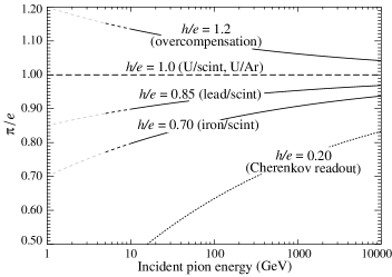
Figure 5: Energy dependence of $\pi/e$ expected for several values of $h/e$ with the assumption that $E_{0}=1$ GeV. For almost all calorimeters, $h/e<1$. The value for a given combination (U/scint, etc.) depends on the actual configuration. The lower dotted line, for $h/e\ll 1$, should be applicable to a calorimeter with Cherenkov readout. The power-law description is not expected to be dependable below about 10 GeV, but nonetheless seems adequate at 5 GeV.

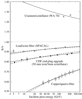
Figure 6: Fits to test-beam results for a lead/scintillator-fiber)[25], for the CDF upgrade end-cap hadron calorimeter (50 mm iron/3 mm scintillator sheets)[26], for a copper/quartz-fiber test calorimeter[13], and for the WA 78 uranium/scintillator calorimeter[20]. Fit parameters are given in Table 1.

Table 1: Power law fits to a variety of $\pi/e$ measurements. The ZEUS uranium/scintillator[23] and D0 U/LAr[24] calorimeters are so close to compensating as to be uninteresting in this context.

Calorimeter	$m$	$a$	$\chi^{2}$	$h/e$*	Expected $h/e$
SPACAL[25]	0.788	0.164	9.2	0.836	0.853–0.895†
(lead/scint-fiber)	0.830 ‡	0.141	14.0	0.859	0.853–0.895†
CDF end-plug had cal[26]	0.865	0.244	2.7	0.756	0.667†
(50 mm Fe/3 mm scint)	0.816 ‡	0.286	14.1	0.714	0.667†
Copper/quartz-fiber[13]	0.833	0.753	2.6	0.247§
(QFCAL)	0.816 ‡	0.814	3.8	0.238
U/scint (WA 78)[20]	0.85♯	$-$0.555♯	–	1.555♯
*Assuming $E_{0}=1$ GeV.
$\dagger$ Paper I, Table 1. (The calorimeters have only approximately the same structure.)
$\ddagger\$Dashed curves in Fig. 6: $m$ held fixed at the value given by the fitted line in Paper I, Fig. 12. Error in $m$ from this work is $\pm 0.01$ to $\pm 0.015$.
$\S$ Akchurin et al. report $e/h\approx 5$[13]. Virtually all of the hadronic Cherenkov signal can be accounted for as coming from relativistic pions[27].
$\sharp$ Ref. [20] gives two data points, shown in Fig. 6. Here I assume $m=0.85$ and adjust $a$ for a best fit.

I emphasize again that the power-law representation is not empirical, but follows from an induction argument. It has the correct asymptotic limit, since $f_{\pi^{0}}^{0}\to 1$ as $E\to\infty$. For a $10^{19}$ eV proton-induced air shower, for example, $f_{\pi^{0}}^{0}\approx 0.98$, in accord with the usual cosmic ray expectation and observation that nearly all the energy deposit at very high energies is electromagnetic. The expected behavior of $\pi/e$ is shown in Fig. 5.

Representative fits of test-beam results to Eq. (7) are shown in Fig. 6. Solid curved are least-squares fits with both $m$ and $a$ allowed to vary, while dashed curves are fits with $m$ is constrained to its nominal value from Paper I. Given the wide range of experimental data which have been fitted to test the power law, one suspects that occasional disparate results (e.g., the low value of $m$ for the CDF end-plug calorimeter) indicate data reduction problems.

Although the energy fraction carried by the nuclear gamma rays scales as the hadronic fraction, it is detected with efficiency $e$ (nearly). Let $f_{\gamma}$ be the fraction of the hadronic energy deposited by nuclear gamma rays within the electronic gate time. Its mean, $f^{0}_{\gamma}$, is independent of both incident hadron energy and species via the “universal spectrum” concept developed in Paper I. Thus $f_{h}\,f_{\gamma}$ of the incident energy is detected with efficiency $e$, and the total em fraction $f_{\rm em}$ is $f_{\pi^{0}}+f_{h}\,f_{\gamma}$. The remaining $f_{h}\,(1-f_{\gamma})$ is detected with redefined hadronic detection efficiency $h^{\prime}$. Then

$$\pi/e= (f^{0}_{\pi^{0}}+f^{0}_{h}f^{0}_{\gamma})+(h^{\prime}/e)f^{0}_{h}(1-f^{0}_{\gamma})$$

$$= 1-\left(1-h^{\prime}/e)(1-f^{0}_{\gamma}\right)f^{0}_{h}$$

$$\approx 1-\left(1-h^{\prime}/e)(1-f^{0}_{\gamma}\right)(E/E_{0})^{m-1}$$

$$\equiv 1-a\,E^{m-1}\ ,$$ (8)

where, as elsewhere, the superscript zero indicates the mean.

The important point here is that the power-law description given by Eq. 7 is recovered, even though part of the electromagnetic signal tracks with the hadronic sector. It is immaterial whether we use $(1-h/e)$ or $(1-h^{\prime}/e)(1-f^{0}_{\gamma})$, except that we should remember that $h$ contains a nuclear gamma-ray component.

Energy deposit by nuclear gamma rays can account for 10%–20% of the total energy deposit in materials such as iron, and it can be even higher in high-$Z$ materials[17]. Since most of the nuclear de-excitations are the result of slow neutron capture, nearly all of the gamma rays are emitted on a time scale of hundreds of ns (see Fig. 3.22 in Ref. [3]). Electronic gate widths for calorimeter signals are made as short as possible, given the arrival time spread of information in such large devices, and this turns out to be close to 100 ns. This means that most of the nuclear gamma energy deposit happens outside of the sampling time. There are a few gammas from faster neutron captures, but by and large most of the gamma signal is lost. Thus $f_{\gamma}$ as defined above is in the range of a few percent. While the above development is of interest in showing that the power-law scaling does not need modification, it is of not much practical importance.

4 $\pi$/p

We observed in Paper I that $f_{\pi^{0}}^{0}$ is larger for an incident charged pion than for an incident proton (or neutron). This is a consequence of the fact that a leading hadron, carrying a large fraction of the energy, is likely to have the same quark number as the incident hadron. If the collision is instigated by a charged pion, there is high probability that the leading hadron is a $\pi^{0}$, but for an incident proton or neutron the leading hadron is most likely a baryon.

Figure 7: Expected $\pi/p$ for one of the SDC reconfigurable absorber test-beam configurations [28] in which $h/e\approx 0.67$. $m$, $E_{0\pi}$, and $E_{0p}$ are from the fits shown in Fig. 11 of Paper I.

Via the “universal spectrum” concept we expect that the hadronic response of the calorimeter is the same for protons as for pions, except for a scale factor: $h/e$ is the same for both cases, and the mean hadronic fraction ratio $f^{0}_{\pi^{-}}/f_{p}^{0}<1$ is independent of energy. These statements are independent of a power-law approximation.

In the power-law context, the energy-independent ratio $f^{0}_{\pi^{-}}/f_{p}^{0}$ should be $(E_{0\pi^{-}}/E_{0p})^{1-m}$. This means that $m$ is the same for both pions and protons. The Paper I (Fig. 11) simulations were consistent with equality. The scale energy $E_{0\pi^{-}}$ was found to be about 1 GeV, with some change from material to material. For protons the Monte Carlo simulations yielded $E_{p0}\approx 2.6$ GeV. These were consistent with the expectation that $E_{0}$ was the approximate multiple-pion threshold[2]. Thus $f_{\pi^{-}}^{0}/f_{p}^{0}\approx(1.0/2.6)^{1-m}=0.83$ for $m=0.815$ and $f_{p}^{0}/f_{\pi}^{0}=0.87$ for $m=0.85$.

If $h/e\neq 1$, a calorimeter should give a different response for charged pions than for protons. In the usual case, where $h/e<1$, pions give the larger response. The effect is illustrated in Fig. 7, where as an example we use $h/e=0.67$, obtained from CALOR simulations (Paper I, Table 1) for the “iron” configuration of the SDC test-beam calorimeter[28]. It is regrettable that there was not time to measure the effect there.

Equation (6) may be rewritten for the pion and proton cases:

$$\pi/e =1-(1-h/e)f_{\pi^{-}}^{0}$$

$$p/e =1-(1-h/e)f_{p}^{0}$$ (9)

Rearrangement gives us the energy-independent ratio of the energy-dependent mean hadronic fractions:

$$f_{\pi^{-}}^{0}/f_{p}^{0}= \frac{1-\pi/e}{1-p/e}$$ (10)

$$\phantom{f_{\pi^{-}}^{0}/f_{p}^{0}}\approx (E_{0\pi^{-}}/E_{0p})^{1-m}$$ (11)

The factor $(1-h/e)$ cancels. The constant ratios of energy-dependent quantities given by Eq. 11 does not depend upon a power law or any other model for the hadronic fractions, although the statistical sensitivity is maximal for small $h/e$.

Specialization to the power-law case results in Eq. 11. Since only $a=(1/h/e)E_{0}^{1-m}$ can be found from $\pi/e$ (or $p/e$) measurements, the scale energy cannot be found without assumptions about $h/e$. It is therefore interesting that the ratio of the scale energies given by Eq. 11 can be very well known.

Table 2: Calculation of the hadronic fraction ratio $f_{\pi^{-}}^{0}(E)/f_{p}^{0}(E)$ as a function of incident hadron energy (last column) using Eq. (11) and data from Table 2 of Akchurin et al.[14]. $\left\langle f_{\pi^{-}}^{0}/f_{p}^{0}\right\rangle=0.859\pm 0.004$, with $\chi^{2}=13.2$. Most of $\chi^{2}$ is contributed by the first and third points.

Energy	Response[14]		$f_{\pi^{-}}^{0}/f_{p}^{0}$
(GeV)	$p/e$	$\pi/e$
200	$0.562\pm 0.013$	$0.647\pm 0.001$	$0.806\pm 0.024$
250	$0.580\pm 0.010$	$0.648\pm 0.001$	$0.838\pm 0.020$
300	$0.590\pm 0.006$	$0.658\pm 0.001$	$0.834\pm 0.012$
325	$0.592\pm 0.006$	$0.652\pm 0.001$	$0.853\pm 0.013$
350	$0.607^{+0.001}_{-0.004}$	$0.659\pm 0.001$	$0.868\pm 0.007$
375	$0.611^{+0.001}_{-0.003}$	$0.664\pm 0.001$	$0.864\pm 0.005$

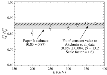
Figure 8: The mean hadronic fraction ratio $f_{\pi^{-}}^{0}/f_{p}^{0}$ as calculated from the copper/quartz-fiber calorimeter data of Ref. [14]. The gray band is the range expected from Paper I; the crosshatched band is a constant value fitted to the data. The PDG scale factor is 1.6.

Since Paper I was published, the CMS forward calorimeter group at CERN has measured the $\pi/p$ ratio using a calorimeter consisting of quartz fibers embedded in a copper matrix (QFCAL)[13, 14]. In this calorimeter, only light was detected, most of it coming from em showers, so that $h/e$ was small, and the $\pi$–$p$ response difference was maximal. $\pi/e$ and $p/e$ as a function of energy are reported in Table 2 of Ref. [14] and copied to our Table 2.

This ratio is calculated in the right column of Table 2 for the Akchurin et al. data. These data together with estimates of the Paper I and a least squares fit to a constant $f_{\pi^{-}}^{0}/f_{p}^{0}$ are shown in Fig. 8. The fit yields $f_{\pi^{-}}^{0}/f_{p}^{0}\approx 0.86$.

I am unable to find flaws in the several arguments leading to the conclusion that $f_{\pi^{-}}^{0}(E)/f_{p}^{0}(E)$ is independent of energy, yet Fig. 8 shows evidence for energy dependence. A straight line with nonzero slope would certainly fit the data better than a constant value. Akchurin et al.[14] needed to make a careful but difficult subtraction of $\pi^{+}$ contamination in their positive beam. The contamination was minimal at the highest energy, as is reflected in the uncertainties. If the pion contamination correction were overdone, one would obtain the observed low values at the lower energies.

In the case of incident kaons, the leading hadron is probably a strange meson, but sometimes a pion. It is unlikely to be a proton or neutron. The response difference between incident pions and kaons should thus be small.

5 mips

As indicated above and in Fig. 1, $e$ and $h$ are the efficiencies with which electromagnetic and hadronic energy are converted into a visible signal. It is conventional to scale signal sizes, in ADC counts, to the mean response for minimum ionizing particles (mips), thus giving them something of an absolute meaning. In practice the “average” signal from penetrating muons, corrected for radiative losses, is assumed to be described by the Bethe-Bloch equation including the density effect. It is then scaled to the value at minimum ionization, presumably defining the mip.

But the mip is commonly used incorrectly.

In a simplification of the normal derivation of the Bethe-Bloch formula, ionization and excitation energy losses are calculated separately for (soft) distant collisions (low energy transfer per interaction) and (hard) near collisions (high energy transfer). The regions are distinguished by the approximations appropriate to each[29, 30, 31]. One hopes for an energy at which they meet; this can sometimes be a problem in high-$Z$ materials. Each contributes a factor $\ln\beta\gamma$ to the behavior at high energies:

1. As the particle becomes more relativistic, its electric field flattens and becomes more extended. This extension is limited by polarization of the material. This “density effect” asymptotically removes the $\ln\beta\gamma$ factor contributed by the distant-collision region. The “relativistic rise” is still there, but with half the slope[32].

2. The kinematic maximum energy $T_{\rm max}$ which can be transferred in one collision sets the upper limit for hard energy transfer. Its rise with energy is responsible for the other $\ln\beta\gamma$ factor. As the particle energy increases there is more $\delta$-ray production and the “Landau tail” grows and extends. The most probable energy loss, in a region well below minimum ionization that is dominated by many soft collisions, shows little or no relativistic rise and approaches a “Fermi plateau.” This is more easily understood for the related restricted mean energy loss discussed below.

 The $\delta$ rays are part of energy loss as described by the Bethe-Bloch equation, and must not be confused with the density-effect correction $\delta(\beta\gamma)$ or the muon radiative processes discussed below.

For detectors of moderate thickness $x$ (e.g., the scintillator tiles or LAr cells used in calorimeters), the energy-loss probability distribution $f(\Delta;\beta\gamma,x)$ is adequately described by the Landau (or Landau-Vavilov-Bichsel) disitribution[33, 34, 35]. The most probable energy loss is

$$\Delta_{p}=\xi\left[\ln\frac{2mc^{2}\beta^{2}\gamma^{2}}{I}+\ln\frac{\xi}{I}+j-\beta^{2}-\delta(\beta\gamma)\right]\ ,$$ (12)

where $\xi=0.153537\left\langle Z/A\right\rangle(x/\beta^{2})$ MeV for a detector with a thickness $x$ in g cm^-2, and $j=0.200$. While $dE/dx$ is independent of thickness, $\Delta_{p}/x$ scales as $a\ln x+b$. The density correction $\delta(\beta\gamma)$ was not included in Landau’s or Vavilov’s work, but it was later included by Bichsel[34]. It must be present for the reasons discussed in item (1) above. The high-energy behavior of $\delta(\beta\gamma)$ is such that

$$\Delta_{p}\mathop{\longrightarrow}_{\beta\gamma{\mathrel{\hbox to0.0pt{\raise 1.5401pt\hbox{$>$}\hss}{\lower 1.5401pt\hbox{$\sim$}}}}100}\xi\left[\ln\frac{2mc^{2}\xi}{(\hbar\omega_{p})^{2}}+j\right]\ ,$$ (13)

where $\hbar\omega_{p}$ is the plasma energy in the material, 21.8 eV in the case of polystyrene[RPP06, Tab. 27.1]. Thus the Landau most probable energy loss, like the restricted energy loss, reaches a Fermi plateau. The Bethe-Bloch $dE/dx$ and Landau-Vavilov-Bichsel $\Delta_{p}/x$ in polystyrene (scintillator) are shown as a function of muon energy in Fig. 9. It is interesting that the asymptote is nearly reached at 10 GeV for muons, and that it is not much higher than the minimum at just under 1 GeV.

In the case of restricted energy loss [RPP06 Eq. (27.2)] the maximum kinetic energy transfer in a single collision is limited to some $T_{\rm cut}\leq T_{\rm max}$. One may find the energy-weighted integral of the $\delta$-ray spectrum ($d^{2}N/dxdT$; RPP06 Eq. (27.5) ) between $T_{\rm cut}$ and $T_{\rm max}$ to find that it is equal to the difference between the restricted and Bethe-Bloch energy-loss rates. Similarly, one can integrate the $\delta$-ray distribution over energy to find the number of $\delta$ rays produced in a tile—to find that in most cases $x\,dN/dx\ll 1$. As the incident particle energy increases, the tail of the Landau distribution contains increasingly energetic but improbable energy transfers. Examples are shown in Fig. 9.

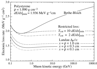
Figure 9: Bethe-Bloch $dE/dx$, two examples of restricted energy-loss rate, and the Landau most probable energy deposit per unit thickness in polystyrene scintillator, in which $dE/dx|_{\rm min}=1.936$ MeV g${}^{-1}\,$cm². The incident particles are muons.

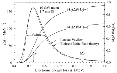
Figure 10: Bichsel’s calculations of the electronic energy deposit distribution for a 10 GeV muon traversing a 1.7 mm silicon detector (which has roughly the stopping power of a 3-mm thick scintillator)[34, 37, 38, 39]. The Landau-Vavilov function (dot-dashed) uses a Rutherford cross section without atomic binding corrections but with a maximum kinetic energy transfer limit $T_{\rm max}$. The solid curve was calculated using Bethe-Fano theory. $M_{0}(\Delta)$ and $M_{1}(\Delta)$ are the cumulative 0th and 1st moments of $f(\Delta)$, respectively. The fwhm of the Landau-Vavilov function is about $4\xi$ for detectors of moderate thickness. $\Delta_{p}$ is the most probable energy loss, and $\left\langle\Delta\right\rangle$ divided by the thickness is the Bethe-Bloch mean, $dE/dx$.

In summary: The mean of the energy loss given by the Bethe-Bloch equation is ill-defined experimentally and is not useful for describing energy loss by single particles. (It probably finds its best application in dosimetry, where only bulk deposit is of relevance.) It rises with energy because $T_{\rm max}$ increases. The large single-collision energy transfers that increasingly extend the long tail are rare.

For a $\beta\approx 1$ particle, for example, on average only one collision with $T>1$ keV will occur along a path length of 90 cm of Ar gas[39]. The energy-loss distribution for a 10 GeV muon traversing a 1.7 mm silicon detector, shown in Fig. 10, further illustrates the point. Here about 90% of the area ($M_{0}(\Delta)/M_{0}(\infty)$) but only $\sim 60\%$ of the energy deposition ($M_{1}(\Delta)/M_{1}(\infty)$) falls below the Bethe-Bloch $\left\langle\Delta\right\rangle$, and at this energy $\Delta_{p}\approx 0.6\left\langle\Delta\right\rangle$. The long tail of $f(\Delta)$ extends to $T_{\rm max}=4800$ MeV.

The mean of an experimental sample consisting of a few hundred events is subject to these large fluctuations, sensitive to cuts, and sensitive to background. The mean $\left\langle\Delta\right\rangle_{\rm exp}$ deduced from the data will almost certainly underestimate the true mean; in general $\Delta_{p}<\left\langle\Delta\right\rangle_{\rm exp}<\left\langle\Delta\right\rangle$. On the other hand, fits to the region around the stable peak in the pulse-height distribution provide a robust determination of the most probable energy loss. The peak is somewhat increased from the Landau $\Delta_{p}$ by experimental resolution function.

The ionization/excitation energy fraction sampled by the active region is conventionally given by

$$\hbox{fraction sampled}=\frac{S\,dE/dx|_{\rm scint}}{S\,dE/dx|_{\rm scint}+A\,dE/dx|_{\rm abs}}\ .$$ (14)

Boundary-crossing $\delta$ rays are (accurately) assumed not to be important. Here $S$ is the active region thickness, $dE/dx|_{\rm scint}$ is the energy loss rate in the active region (scintillator or other), $A$ is the absorber thickness, and $dE/dx|_{\rm abs}$ is the energy-loss rate in the absorber. It is “fairly sampled” if this is the case. It is not the case for electron and muon radiative losses.

Relativistic muons also lose energy radiatively by direct pair production, bremsstrahlung, and photonuclear interactions. In iron at 1 TeV, these loss rates are in the ratios 0.58:0.39:0.03. The ratios are fairly insensitive to energy at energies where the radiation contribution is important. The pair:bremsstrahlung ratio is about the same from material to material, while the photonuclear fraction grows with atomic number. These contributions to $dE/dx$ rise almost linearly with energy, becoming as important as ionization losses at some “muon critical energy” $E_{\mu c}$: 1183 GeV in plastic scintillator, 347 GeV in iron and 141 GeV in lead.

The tables of Lohmann et al.[40] are commonly used. More extensive tables with a somewhat improved treatment of radiative losses are given by Groom et al.[31], and an extension to nearly 300 materials is available on the Particle Data Group web pages[41].

Muons in an absorber are accompanied by an entourage of photons and electrons (cascade products from direct pair production and bremsstrahlung) characteristic of radiative losses in the higher-$Z$ absorber. If the calibration muon beam has been momentum-selected and then travels through air or vacuum to the calorimeter, it enters “naked,” without its entourage of pairs and bremsstrahlung photons and, until this builds up over several radiation lengths, the signal distribution does not include the full radiation contribution. If the equilibrium contribution is desired, absorber should be placed in the beam. In principle these radiative products should be detected with the same efficiency as electrons, although a few high-energy pairs go through the active layers. There is little radiative loss in the low-$Z$ active layers themselves.

Bremsstrahlung is sufficiently continuous as to not introduce significant radiation fluctuations[42], but there are large fluctuations in the pair production energy loss. Monte Carlo calculations by Striganov and collaborators[43] indicate that, while a high-energy shoulder appears on the energy-loss distribution, the most probable energy loss increases only slightly in “thin” absorbers,” e. g. for 1000 GeV muons incident on 100 g cm^-2 of iron. They regard radiative effects as “important” when the most probable height of the normalized energy-loss distributions are lowered by $\mathrel{\hbox to0.0pt{\raise 2.20013pt\hbox{$>$}\hss}{\lower 2.20013pt\hbox{$\sim$}}}10$% when radiative effects are included. This is the case for the total signal from real calorimeters (more than 1000 g cm^-2) at the highest muon calibration energies normally used. Although the most probable energy loss is still the best calibration metric, it does rise somewhat with beam energy because of the radiative effects.

The calibration of the HELIOS modules (uranium/scintillator sandwiches) is particularly well described[44]. The common normalization of individual layers was done via radioactive decay in the uranium plates, so the distributions shown are for entire modules. In correcting for the radiative losses they assumed fair sampling by the scintillator. Their correction of energy deposit for radiative effects is straightforward, but the robustness of the “average” energy deposit is unclear.

Muon detection in SPACAL (scintillator fibers in a lead matrix) is carefully described by Acosta et al.[45]. The energy dependence of the most probable values is shown. The distributions clearly show both the radiative broadening and the increase of the most probable values due to radiative effects.

In both of these cases, the calorimeters as a whole were calibrated. Since these are many radiation lengths thick, the lower average deposit at the beginning should not sensibly affect the result.

All of this assumes muons of known energy. “Out of channel” muons, which have gone through or around the test-beam optics, are certainly not dependable calibration particles, but are sometimes used[28]. Cosmic ray muons have a characteristic energy of about 3 GeV, but the flux falls off as about $\cos^{2}\theta$, where $\theta$ is the zenith angle [RPP06, Sec. 24]. They can provide a useful if imprecise calibration in some situations.

6 e, h, and e/h

Given a credible muon calibration, the quantity $e/mip$ can be measured in an electron beam. In a sampling calorimeter, cascade electrons are predominately produced and absorbed in the inactive higher-$Z$ material, so the signal is significantly smaller than might be expected from the active layer’s share of $dE/dx$ ($e/mip\approx 0.6$ to 0.7[46]), but with uncertainty associated with most probable energy deposit vs average energy deposit. It can be “tuned” by changing the absorber/detector ratio, perhaps to achieve compensation ($h/e=1$). Other things being equal, the detection efficiency is smaller if the absorber has a higher $Z$. The critical energy is lower, so characteristic shower electrons are more likely to deposit their energy before leaving the absorber. As a corollary, $e/mip=1$ for a nonsegmented calorimeter (e.g., an inorganic crystal), and since there is always missing hadronic energy such a calorimeter is always noncompensating.

The hadron efficiency $h$ is more problematical; one finds $a=(1-h/e)E_{0}^{1-m}$ or an equivalent by fitting the energy dependence of $\pi/e$, and assumptions must always be made about the constant multiplier to find $h/e$ and hence $h/mip$. The multiplier $E_{0}^{1-m}$ is close to 1 for incident pions, but it is about 20% higher for protons. $h$ is considerably more difficult to model, but in general it is smaller than $e$ because of the wide variety of ways hadronic energy becomes invisible, e.g., through nuclear binding energy losses and “late” energy deposition (outside the electronics window). It increases somewhat with $Z$, and can be enhanced by neutron production in uranium. It can also be “tuned” by the choice of material and sampling fraction[3].

Can we measure $h/mip$ directly? Only by observing hadronic cascades in a calorimeter insensitive to $\pi^{0}$-produced em cascades, or by observing cascades produced by hadrons below the $\pi^{0}$ threshold. In Paper I we speculated about building a calorimeter sensitive only to hadrons (a neutron detector) or to the em sector (a calorimeter sensitive only to Cherenkov radiation), but the context of the discussion was verification of the power-law approximation for $f^{0}_{h}$ and determination of the power $m$.

In the spirit of only- (mostly-) em sensitivity in the copper/quartz-fiber CMS test calorimeter, Demianov et al.[47] made preliminary neutron measurements using Bonner spheres[48] adjacent to the copper/quartz-fiber calorimeter[13]. The longitudinal and transverse distributions were measured. The results were in fair to good agreement with MARS96[49] calculations, but not sufficiently detailed to obtain $h/mip$ (or $n/mip$). Preliminary proposals[50] (in connection with International Linear Collider (ILC) detector R&D) are being made to measure the neutron flux by a variety of methods; future test-beam results will be of great interest. The problem will be discussed at more length in Sec. 9.

One might use hadrons with energies below the $\pi^{0}$ threshold. ZEUS collaborators made measurements with low-energy protons and charged pions with a compensated U/scintillator calorimeter[51]. Interestingly, as the kinetic energy of the beam was decreased from about 5 GeV to about 0.4 GeV, $e/h$ decreased from its high-energy value (one) to the $e/mip$ measured for electrons. The lower-energy particles tended to lose much or all of their energy by ionization, so they became indistinguishable from electrons at sufficiently low energies. The resolution also decreased from its hadronic value, approaching the em resolution until at the lowest energies noise became dominant.

A more desirable (or complimentary) approach might be to use an incident beam of low-energy neutrons. Since $E_{0p}\approx 2.6$ GeV, one might expect the $\pi^{0}$ threshold to be about $T\approx 1.6$ GeV. As the energy is scanned downward, a pure hadronic signal should emerge. The response would not be quite the hadronic signal observed from a higher-energy cascade, but this difference can probably be understood. At very least, measurements in a low-energy neutron beam would be interesting. The real problem is making the test beam.

7 Resolution

The arrows between boxes in Fig. 1 actually indicate the various p.d.f.’s describing fluctuations in each of the steps. A more complete version, Fig. 11, defines these distributions, which are described in more detail in Table 5. In the simple model considered in this paper, five p.d.f.’s appear.

The potentially detectable energy deposit, or visible energy, is labeled “vis.” It usually means ionization in a sensing medium, such as scintillator or liquid argon. In the rare cases where Cherenkov light is to be sampled, it means the Cherenkov radiation produced. It contains the variations due to energy deposit, not detection. The variance associated with the visible energy distribution at fixed $E_{\pi^{0}}$, dominated by fluctuations in the total kinetic energy of neutrons, is the intrinsic variance.

This ionization is then sampled directly but more often via scintillators, where the scintillation light is usually detected by photomultipliers. The label “samp” refers to the additional fluctuations introduced in this process.

The stochastic processes are defined as follows:

1. In the cascade initiated by the incident hadron, energy $E_{\pi^{0}}$ is transferred to the $\pi^{0}$ sector via $\pi^{0}$ production and decay. Because of its different energy dependence, em energy deposited by nuclear gamma rays is not included in my definition of $E_{\pi^{0}}$. The p.d.f. $\Pi(E_{\pi^{0}})$ was introduced in Sec. 2 to describe its distribution.

2. The ${\pi^{0}}$ energy $E_{\pi^{0}}$ is detectable with some average efficiency $e$ via the ionization produced mostly by low-energy electrons and positrons. The p.d.f. of the em visible energy deposit at fixed $E_{\pi^{0}}$ is labeled $g_{\pi^{0}}(E^{\rm vis}_{\pi^{0}}|E_{\pi^{0}})$.

3. Quite independently, the hadronic component produces a visible signal via energy loss by charged secondaries. This signal, the result of a variety of mechanisms, is produced with an overall average efficiency $h$. The visible contribution by nuclear gamma rays is included here. Again, most of the ionization is by low-energy particles. The p.d.f. $g_{h}(E^{\rm vis}_{h}|E_{\pi^{0}})$ describes the distribution at fixed $E_{\pi^{0}}$.

4. Only the total deposit $E^{\rm vis}=E^{\rm vis}_{\pi^{0}}+E^{\rm vis}_{h}$ can be detected. Convolution over the intermediate variable $E^{\rm vis}_{\pi^{0}}$ yields the p.d.f. $F_{\rm vis}(E^{\rm vis}|E_{\pi^{0}})$. The product of this distribution with $\Pi(E_{\pi^{0}})$, integrated over $E_{\pi^{0}}$, is the visible energy distribution which can be sampled. The width of this distribution is identified with the “intrinsic resolution.”

   

   
   

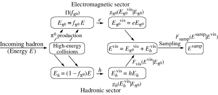
   Figure 11: Energy flow in a calorimeter, with the statistical distributions contributing to the experimental resolution indicated.

5. Finally, the visible energy is sampled by measuring the ionization, either directly or by observing scintillation light with photomultipliers or photodiodes. This step is to an extent under the control of the experimenter, since it depends on scintillation efficiency, light collection efficiency, and other design details. For fixed $E^{\rm vis}$ one measures a signal $E^{\rm samp}$, chosen from a distribution $F_{\rm samp}(E^{\rm samp}|E^{\rm vis})$, which is then summed over the intermediate $E^{\rm vis}$ to obtain the final distribution of the signal, $E^{\rm samp}$. Even this step is not a simple convolution, since the variance of $F_{\rm samp}(E^{\rm samp}|E^{\rm vis})$ is proportional to $E^{\rm vis}$, not $E$.

The intrinsic and sampling distributions were separated in a classic experiment by Drews et al.[52], who used compensating sandwich calorimeters with scintillator readout with either lead or uranium plates. Alternate sets of scintillators were read out separately. Sampling variations in the two sets were independent, while intrinsic fluctuations were correlated. These were recovered by adding and subtracting variances.

Calculation of the combined distribution is tedious and not entirely obvious; the details are relegated to Appendix A. The result (repeating Eq. (43)) is

$$\left({\sigma\over E}\right)^{2}=\frac{(\pi/e)\sigma_{\rm samp0}^{2}}{E}+\left[\frac{f_{\pi^{0}}^{0}\sigma_{e0}^{2}}{E}+\frac{f^{0}_{h}\sigma_{h0}^{2}h/e}{E}\right]+(1-h/e)^{2}\sigma_{\pi^{0}}^{2}(E)\ .$$ (15)

Here $\sigma^{2}_{\rm samp0}$, $\sigma^{2}_{e0}$, and $\sigma^{2}_{h0}$ scale the variances contributed by the sampling, $\pi^{0}$ energy deposit, and hadronic energy deposit, respectively. They have the units of energy.

The first term is the familiar sampling contribution, except that it is multiplied by $\pi/e$. This is to be expected and required, since this contribution to the variance is proportional to the sampled visible signal, with mean $(\pi/e)E$, rather than to the incident energy $E$.

The two terms in the square brackets are the two pieces of the intrinsic variance. Even if $h/e=1$, the intrinsic variance has some energy dependence, since $f_{\pi^{0}}$ increases with energy and $f_{h}$ decreases with energy.

Together, the sampling term and the two intrinsic terms in the square brackets are usually represented as $(C/\sqrt{E})^{2}$, ignoring the energy dependence of each of the three terms.

Wigmans[3] has noted that $\sigma_{\rm intr}/\sqrt{E}$ for the simulated lead/LAr calorimeter described in his Table 3.4 decreases with energy, reflecting the gradually increasing transfer of energy to the ${\pi^{0}}$ sector. His calculated results for six energies, given in his Table 4.3, are plotted in Fig. 12. My curve was obtained by adjusting the intrinsic variance scales $\sigma^{2}_{e0}$ and $\sigma^{2}_{h0}$. The best-fit parameters are $\sigma_{e0}=5.1\%$ and $\sigma_{h0}=13.7\%$. The fit is remarkably good, and, as expected, $\sigma_{h0}$ is considerably larger than $\sigma_{e0}$.

Figure 12: Wigman’s (simulated) data[3] for the intrinsic resolution of a Pb/LAr calorimeter scaled by $1/\sqrt{E}$, fitted with the term in the square brackets of Eq. (15). The fit parameter are given in the text.

The last term is the expected “constant term.” Its mild energy dependence is discussed in Sec. 2. It must approach zero at high energies ($1/E\to 0$), as $\Pi(f_{\pi^{0}})$ “crowds against” the $f_{\pi^{0}}=1$ limit. That it can be represented as a constant is an artifact of the limited energy range of test-beam measurements. This point is discussed in more detail below.

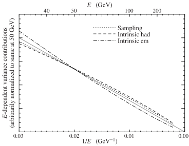
Figure 13: Shapes of contributions to sampling and intrinsic variance. As $1/E\to 0$, the slopes of the sampling and ${\pi^{0}}$contributions approach finite constants, since $\pi/e\to 1$ and $f_{\pi^{0}}\to 1$, while the slope of the intrinsic hadronic contribution approaches zero ($f_{h}\to 0$).

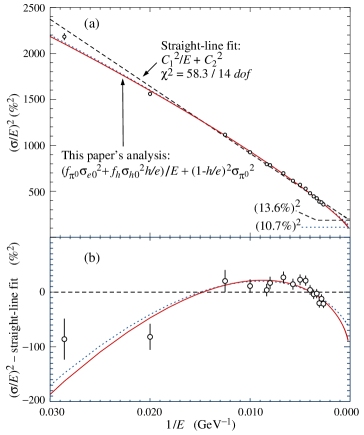
Figure 14: “Conventional” and Eq. (15) fits to the copper/quartz-fiber test module energy response data given in Table 3 of Ref. [13]. The fit parameters are given in Table LABEL:tab:fitparameters. The fit shown by the dotted curve is for constant $\sigma_{\pi^{0}}$, while the solid curve fit is for a more physically reasonable weak negative power law $E$-dependence. The high-energy “turndown” is more clearly shown in (b), where the fits and data are shown relative to the usual straight-line fit.

The $\pi^{0}$ part of the intrinsic variance fraction increases in importance as $E$ increases, as does the sampling variance. Both curve downward if plotted vs $1/E$, as shown in Fig. 13. The hadronic intrinsic contribution curves upward, since it decreases faster than $1/E$.

It is difficult to verify Eq. (15), even with robust experimental data. The expected resolution should be a linear combination of the three curves shown in Fig. 13 (plus a constant term), so any deviation of the variance from the traditional $C_{1}^{2}/E$ will show up as a slight curvature. Moreover, the sampling and $\pi^{0}$ contributions have such similar energy dependence that a simultaneous fit to $\sigma_{\rm samp0}$ and $\sigma_{e0}$ can be indeterminate.

Table 3: Parameters for the three fits shown in Fig. 14. The power-law parameters $m=0.833$, $a=0.753$ and $h/e=0.247$ (for $E_{0}=1.0$) from Table 1 were used in the reduction. The experimental data are from the 3rd ($\sigma_{\rm rms}/E)$ column of Tbl. 3 in Ref. [13].

$\sigma/E=C_{1}/\sqrt{E}\oplus C_{2}$			Eq. (15) with $\sigma_{\rm samp0}=0$			Eq. (15) with $\sigma_{\rm samp0}=0$
Parameter	Value		Parameter	Value		Parameter	Value
			$\sigma_{e0}$	377%		$\sigma_{e0}$	372%
$C_{1}$	270%		$\sigma_{h0}$	216%		$\sigma_{h0}$	214%
			$s_{1}*$	14.2%		$s_{1}*$	15.7%
			$s_{2}*$	0 (fixed)		$s_{2}*$	$-$0.058
$C_{2}$	13.6%		$(1-h/e)s_{1}$	10.7%
$\chi^{2}/dof$	58.3/14		$\chi^{2}/dof$	18.6/13		$\chi^{2}/dof$	18.0/12
* $\sigma_{\pi^{0}}=s_{1}\,(E/100\,{\rm GeV})^{s_{2}}$

The square of the fractional energy resolution in the copper/quartz-fiber test calorimeter for incident pions (Akchurin et al.[13], Table 3) is plotted as a function of $1/E$ in Fig. 14. The data curve downward relative to the “conventional” linear fit, $C_{1}^{2}/E+C_{2}^{2}$, shown by the dashed line. For this calorimeter intrinsic fluctuations were more important than sampling fluctuations except at the lowest energies, although sampling fluctuations were not negligible. Because of the nearly-degenerate shapes of the sampling and intrinsic $\pi^{0}$ fluctuation curves, I set $\sigma_{\rm samp0}=0$ in making a fit, which is shown by the solid curve in the Figure. It describes the data well, and the physics responsible for the curvature is understood.

Parameters for both cases are shown in Table LABEL:tab:fitparameters. The fitted values for $\sigma_{e0}$ and $\sigma_{h0}$ are very much larger than for the example discussed above and shown in Fig. 12; this follows from the excellent resolution of Wigman’s model calorimeter and the (by design) poor resolution of the copper/quartz-fiber calorimeter.

Other examples testing the $1/E$ dependence are hard to find. Many test-beam results are at low energy, many have large errors, and many of the earlier results are presented as functions of $C_{1}/\sqrt{E}+C_{2}$ rather than $C_{1}/\sqrt{E}\oplus C_{2}$. It will be of interest to test Eq. (15) against further experimental results.

8 Jets

How is calorimeter’s response to a jet different than its response to a single pion? There are three situations to consider:

1. An incident pion. The primary collision usually occurs about an interaction length into the calorimeter. There is a minimum of backscatter (“albedo”). The fragmentation process is dependent on energy and the nuclear environment.

2. A “test-beam jet,” in which trigger counters ensure that the primary interaction occurs in a thin absorber in front of the calorimeter. This is exactly the same as the incident pion case, except for increased albedo because of the high probability that some of the first-collision debris interacts near the front of the calorimeter.

3. A primary fragmentation jet. The only evident differences from the above cases are the (much) higher energies and a simpler environment; except in heavy-ion collisions just two particles interact. This section concerns whether the mix and distribution of photons, pions, and other particles results in calorimeter response different than the response to a pion or “test-beam jet.”

As elsewhere in this paper, the situation is highly idealized: The homogeneous or fine-sampling calorimeter is large enough to contain the entire cascade and the structure is uniform throughout. The realities of jet-finding and isolation algorithms, albedo, the effects of the magnetic field, passive material in front of the calorimeter, etc., are all ignored.

The power law approximation for $f_{h}$ developed in Paper I will be used throughout this section.

A jet with energy $E_{J}$ consists of photons, mostly from $\pi^{0}$ decay, and “stable” hadrons. (Energy which might be carried away by leptons is ignored.) Since most of the incident “stable” hadron flux consists of charged pions, $E_{0}\approx 1$ GeV and $(1-h/e)\approx a$.

One needs only to sum the calorimeter response to all of these particles to obtain the response to a jet. If $R_{{\pi^{0}}j}$ is the response to the $j$th $\pi^{0}$ (with energy $E_{{\pi^{0}}j}$) in the jet and $R_{hk}$ the response to the $k$th stable hadron (with energy $E_{hk}$), then the response to a jet is given by

$$E_{J}^{\rm vis}=\sum_{j=1}^{N_{\pi^{0}}}R_{{\pi^{0}}j}+\sum_{k=1}^{N_{\rm had}}R_{hk}\ .$$ (16)

Using Eqns. (4)–(7) to evaluate $R_{hk}$ and $R_{{\pi^{0}}j}$, this reduces to

$$E_{J}^{\rm vis}=eE_{J}\Big{[}1-a\,E_{J}^{m-1}\sum_{k=1}^{N_{\rm had}}(E_{hk}/E_{J})^{m}\Big{]}\ .$$ (17)

Alternatively, the spectrum of stable hadrons can be described by a fragmentation function $D(z)$, where $z$ is the hadron’s momentum parallel to the jet direction, scaled by the jet’s momentum. In the present study $z$ is treated as the fractional energy, i.e. $z\approx E_{\rm had}/E_{J}$. When the arguments leading to Eq. 17 are repeated, one obtains

$$E_{J}^{\rm vis}=eE_{J}\Big{[}1-a\,E_{J}^{m-1}\int_{0}^{1}z^{m}D(z)dz\Big{]}\ ,$$ (18)

where $D(z)$ describes the spectrum of all hadrons except for the $\pi^{0}$’s.

The sum (Eq. 17) or integral (Eq. 18) thus appears as a correction factor to the normal hadronic response of a calorimeter. If it is unity, the response to a jet is the same as the response to a pion. In any case it is multiplied by $a$, which is usually $<0.3$. The distinction between a single pion and a jet vanishes as the calorimeter becomes more compensated—except, of course, for the albedo, magnetic field, passive material in front of the calorimeter, and cone-cut effects mentioned above.

If the sum or integral is evaluated for $m=0$, the mean stable hadron multiplicity $\left\langle N_{\rm had}\right\rangle$ is obtained. If $m=1$, the result is the mean nonelectromagnetic fraction of the jet’s energy $\left\langle F_{\rm had}\right\rangle$. The desired summation or integral, with $m\approx 0.82$–0.86, is in some sense an interpolation between the two.

In using either experimental or Monte Carlo distributions to evaluate the sum or integral, special treatment of the very low-$z$ region is necessary, as is normalization to an appropriate $\left\langle F_{\rm had}\right\rangle$.

The integral in Eq. 18 is evaluated for four representative cases:

Two experimental results, both with jet energies at or near $M_{Z}/2$. Since the measurements are for charged hadrons, the distributions must be renormalized to include the contributions of such particles as $\Lambda$’s and $K_{L}$’s.

1. Jets from $Z$ decay, as measured by the DELPHI collaboration at LEP[53]. The published fragmentation function is for the entire event, so the function has been normalized downward by a factor of two to describe the individual jets. Data were read from their Fig. 3(b) and extrapolated to $z=0$.

2. CDF charged fragmentation function at $\sqrt{s}=1800$ GeV[54]. $zdN_{\rm ch}/dz$ was extrapolated to $z=0$ to force $\left\langle F_{\rm ch}\right\rangle=0.65$, their reported value. (Since some of the energy is carried by neutrals, this value is probably too high for consistency with isospin conservation.)

Two samples of TWOJET ISAJET[55] events at $\sqrt{s}=40$ TeV. In both cases, all hadrons other than $\pi^{0}$’s are used:

1. 3226 events with $p_{t}$ (hard scatter) $>40$ GeV/$c$, and $(100\ \hbox{GeV}<M_{JJ}<200\ \hbox{GeV})$. The mean jet momentum is 73 GeV/$c$, and the mean non-$\pi^{0}$ hadronic multiplicity is 26.

2. 3042 events with $p_{t}$ (hard scatter) $>400~{}{\rm GeV/}c$, and $1000\ \hbox{GeV}<M_{JJ}<2000\ \hbox{GeV}$. The mean jet momentum is 677 GeV/$c$, and the mean non-$\pi^{0}$ hadronic multiplicity is 70. The $z$ distribution for these events is shown in Fig. 15.

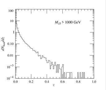
Figure 15: Distribution in $z$ for ISAJET TWOJET events at $\sqrt{s}=40$ TeV, for $1000\ \hbox{GeV}\ <M_{JJ}<2000\ \hbox{GeV}$.

The results are summarized in Table 4. There is ambiguity because of uncertainty in $\left\langle F_{\rm had}\right\rangle$ in the simulations and $\left\langle F_{\rm ch}\right\rangle$ in the experimental results. If pion production dominates, one might expect $\left\langle F_{\rm had}\right\rangle\approx 2/3$ from isospin considerations. (In Paper I, we reported fractions closer to 3/4.) Some of the bias can probably be removed by normalizing $\int zD(z)dz$ to 2/3, as indicated by the table entries in parentheses. As can be seen, the integral is slightly less than unity for the similar low-energy LEP and Tevatron fragmentation functions, and it is slightly greater than unity for simulated 40 TeV jets. Values lie between 0.84 and 1.15 before normalization, and 0.92 to 1.06 after normalization—probably well within the uncertainty of the fragmentation functions in either the experimental or Monte Carlo cases. The integrals also change by about 0.05 if $m$ is changed by 0.01, introducing an additional uncertainty which could be as great as 20%. Given the various uncertainties, I conclude that the correction factor for fragmentation jets at the highest-energy colliders should be between 0.85 and 1.15.

Table 4: Integrals over representative fragmentation functions. Numbers in parentheses are calculated for the nonelectromagnetic energy fraction normalized to 0.67. In the case of the DELPHI and CDF results, the unrenormalized energy fraction is for charged hadrons only.

Source	Process	$\int_{0}^{1}D(z)dz$	$\int_{0}^{1}z^{0.86}D(z)dz$	$\int_{0}^{1}zD(z)dz$
DELPHI	$Z\to jet\ jet$	11.0(12.1)	0.84(0.92)	0.61(0.67)
CDF	$\sqrt{s}=1.8$ TeV	17.8⋆(19.9)	0.94(0.97)	0.65(0.67)
ISAJET	40 TeV, $\left\langle p_{J}\right\rangle=73\,\hbox{GeV}/c$	26.2(25.2)	1.04(1.00)	0.69(0.67)
ISAJET	40 TeV, $\left\langle p_{J}\right\rangle=677\,\hbox{GeV}/c$	69.8(64.7)	1.15(1.06)	0.72(0.67)
⋆ The extrapolated low-momentum part of the function contributes 10 to this total.

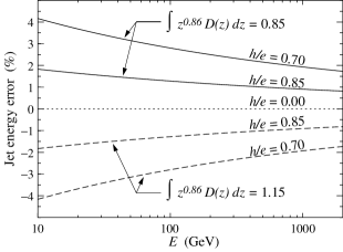
Figure 16: Energy determination error as a function of jet energy for representative values of $h/e$, for the two extreme case of the correction factor: 0.85 (top curves, for hard, low-multiplicity jets) and 1.15 (bottom curves, for soft, high-multiplicity jets).

The compensation factor $a\approx(1-h/e)$ appearing in Eq. (17) and 18 serves to further reduce the effect of the correction factor in producing a $jet/\pi$ difference. The percentage errors for the two limiting cases 0.85 and 1.15 are plotted in Fig. 16 for calorimeters with $h/e=0.70$ and $h/e=0.85$, values which might occur for a Pb/LAr or badly designed metal/scintillator calorimeter. The uncertainty in the exponent $m$ could introduce an error of about 3% for jets below 100 GeV in a poor calorimeter.

In the context of a power law approximation to the hadronic fraction for an incident pion, the response for an incident jet thus differs from the response to an incident pion by a simple correction factor, an integral over the fragmentation function. Given the uncertainties involved, no difference between jet and pion response can be found.

9 Beating the devil

An estimation of the ${\pi^{0}}$ content of individual events would permit correction for intrinsic fluctuations (reduction of the “constant term”), along with its contribution to energy uncertainty.

Several attempts have been made to use the radial and longitudinal detail to estimate, and correct for, the ${\pi^{0}}$-induced cascades. During tests for the SDC construction, it was proposed that the ${\pi^{0}}$ contribution might come “early” in the cascade, and could be estimated by excess energy deposit in the first layers. This turned out not to be true[56]. The ATLAS barrel calorimeter group adjusts downward the contribution of readout cells with large signals, since these tended to be from ${\pi^{0}}$ cascades. In the test-beam runs they achieved slight improvements, e.g., from $(46.9\pm 1.2)\%/\sqrt{E}$ to $(45.2\pm 2.2)\%/\sqrt{E}$[57]. Nearly a decade earlier, this algorithm was successful in correcting the WA 78 data[20]. Ferrari and Sala have simulated such corrections for the LAr TPC ICARUS detector, where very detailed 3D imaging is possible, and conclude that the ${\pi^{0}}$ content can be fairly well determined from the direct observation of the em cascades[17]. The success of these corrections depends on the detail available, and any gains are usually marginal.

Mockett[58] suggested long ago that information from a dual-readout calorimeter with different $h/e$’s in the two channels could be used to estimate the electromagnetic fraction $f_{\pi^{0}}$ for each event. Winn[59] has proposed using “orange” scintillator, observing the ionization contribution through an orange filter and observing the Cherenkov contribution through a blue filter. This has not yet been implemented, and looks problematical.

The idea of using a quartz fiber/scintillator fiber dual readout calorimeter to extract an estimate of $E_{\pi^{0}}$ for each event was discussed by Wigmans in 1997[60]. Since then, the DREAM collaboration(Akchurin et al.[61]) has elegantly demonstrated the efficacy of the dual-readout technique, using a copper/optical fiber test-beam calorimeter. It consists of copper tubes, each containing three plastic scintillator fibers and four undoped fibers which produce only Cherenkov light. These are read out separately for each event.

The principle is illustrated in Fig. 17. Akchurin et al.’s notation is used: $S$ for the scintillator signal and $Q$ for the Cherenkov signal, with both energy scales calibrated with electrons. For this example their values $h/e|_{S}=0.7$ and $h/e|_{Q}=0.2$ are used for the scintillator and nominal Cherenkov readouts respectively. If there were only resolution contributions from the $E_{\pi^{0}}$ distribution, events with different $f_{\pi^{0}}$ should lie along the solid line drawn from $f_{h}=1$ to $f_{h}=0$ ($f_{\pi^{0}}=0$ to $f_{\pi^{0}}=1)$:

$$S=E(f_{\pi^{0}}+f_{h}(h/e|_{S}))\ ,\hbox{\ and}\ \ Q=E(f_{\pi^{0}}+f_{h}(h/e|_{Q}))\ .$$ (19)

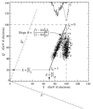
Figure 17: A toy model showing energy correction for 100 GeV pions in an idealized DREAM calorimeter, where $Q$ is the response in the quartz-fiber readout and $S$ is the response in the scintillator-fiber readout. The observed “events” are shown by the +’s, and the corrected events by the $\circ$’s. Rotating to a frame in which the $Q^{\prime}$ axis is parallel to the event locus provides an equivalent reduction.

The effects of finite resolution are illustrated using simulations which give $f_{\pi^{0}}$ for 100 GeV negative pions axially incident on a very large lead cylinder. (Results at 30 GeV from the same study are shown in Fig. 3(a).) For this cartoon example I arbitrarily introduced a Gaussian scatter in both $E_{\pi^{0}}$ ($\sigma_{\pi^{0}}/\sqrt{100~{}\hbox{GeV}}=1.5\%$) and $E_{h}$ ($\sigma_{h}/\sqrt{100~{}\hbox{GeV}}=3.0\%$). The “events” are shown by the small +’s in the figure. The solid histogram at the top shows the marginal distribution in $S$. The mean is 84.7 GeV, the fractional standard deviation is 5.3%, and there is the usual skewness toward high energies.

Energy correction is straightforward. With the definition

$$R=\frac{1-h/e|_{Q}}{1-h/e|_{S}}\ ,$$ (20)

Eq. (19) can be solved to obtain

$$E_{\rm corr}=\frac{RS-Q}{R-1}\ .$$ (21)

The circles in Fig. 17 show the same events after reduction via Eq. (21), and the dashed histogram shows the marginal distribution. The mean is 100.1 GeV, the fractional standard deviation is 3.4%, and there is no evident skewness. Complete compensation has been achieved by using the simultaneous readouts.

Alternatively, a coordinate rotation to axes ($Q^{\prime},S^{\prime}$) can be made, such that the new $Q^{\prime}$ axis is parallel to the event locus. The projection of the event distribution onto the new $S^{\prime}$ axis is of minimal width. Scaled upward by the geometrical factor, it becomes the corrected distribution given by Eq. (21).

The importance of a large “compensation asymmetry” is evident. If the standard deviation in $Q$ is $\sigma_{Q}$ and the standard deviation in $S$ is $\sigma_{S}$ (both in GeV), then the variance in $E_{\rm corr}$ is approximately

$$\sigma_{\rm Ecorr}^{2}=\left(\frac{R}{R-1}\right)^{2}\sigma_{S}^{2}+\left(\frac{1}{R-1}\right)^{2}\sigma_{Q}^{2}$$ (22)

Since $R$ can be well determined either from test-beam measurements of $\pi/e$ as a function of energy or from fits to the slope in a plot of $Q$ vs $S$ at one energy, the error in $R$ has been neglected in writing Eq. (22). In the present example $R=(1-0.2)(1-0.7)=2.66$, so $\sigma_{E}^{2}=3.20\,\sigma_{S}^{2}+0.36\,\sigma_{Q}^{2}$. Given the Cherenkov readout, $\sigma_{Q}^{2}$ is likely to be much larger than $\sigma_{S}^{2}$. The price of the correction is an increased error on each event, but it is clear from Fig. 17 that there is compensating improvement.

Alternate schemes simpler than DREAM would be desirable. Winn’s scheme[59], taking advantage of the different colors of Cherenkov and (red) scintillation light, uses common detectors but still needs the doubled number of photomultipliers. Clean separation of the two signals would likely be difficult. LSND[62] used a weak scintillator and distinguished between directional Cherenkov light and isotropic scintillation light. But this was a very different kind of detector, a homogeneous low-$Z$ detector used in a search for rare signals involving single, low-energy electrons. The electrons at the end of a high-energy shower do not remember the original direction.

Descendants of DREAM are being studied under the rubric of the “Fourth Concept Detector” for the International Linear Collider[63]. One starting point might be the dual-readout quartz/scintillator DREAM concept. It can immediately be improved to get rid of signal correlation between adjacent fibers and simplified, e.g., by alternating scintillator and Cherenkov fibers in groves in sheets of absorber (possibly tungsten) which can then be combined as a sandwich.

An interesting departure from the fiber calorimeter idea was presented by Zhao at a March, 2006 ILC workshop[64]. A “conventional” iron/scintillator-plate sandwich calorimeter is constructed in which lead glass tiles are substituted for all or part of the iron plates. The Cherenkov light is detected via waveshifter fibers in grooves in the tiles. Since lead glass (heavy flint glass) with specific gravities up to about 5.7 are available, the calorimeter thickness might not be that excessive. However, one expects that transverse structure observation is essential, and there remains the problem of neutron detection.

Perhaps a better approach is to observe the fast, blue, directional, polarized Cherenkov light from an inorganic scintillator. This is the object of present test beam work, using the scintillator PbWO₄[27]. (The slow component has only a 50 ns decay time, $\lambda_{\rm max}=560$ nm (yellow), but the scintillation efficiency is only 0.1% that of NaI.)

But if neutron detection can be added to neo-DREAM, then the in-principle ultimate 1% hadron calorimeter resolution[60] might be approached. Ways to do this are under active investigation by the Forth Concept collaborators and others, who hope to exploit one or more distinguishing features of the neutron signal:

1. Neutrons distribute further from the core of a cascade than do other components.

2. Gamma rays from nuclear de-excitation following thermal neutron capture are slow, in the several hundred ns range[3]. Given fast gating requirements, their signal is probably not useful.

3. In a hydrogenous scintillator, ionization from the proton recoils in $n$-$p$ elastic scattering can be observed.

4. Most neutron detectors in nuclear physics take advantage of the large cross sections for the ${}^{10}{\rm B}(n,\alpha)$, ${}^{6}{\rm Li}(n,\alpha)$, and ${}^{3}{\rm He}(n,p)$ reactions, with the boron reaction being the most popular[65]. The gas-filled detectors in common use are impractical for a calorimetric applications, but boron- and lithium-loaded scintillators exist and are being further developed. The inorganic scintillator LiI(Eu) is an obvious candidate, but its crystalline structure and 300 ns decay time both present problems. Organic borate additives in conventional plastic scintillators might have promise. There are common high-boron glasses and there are glass scintillators; whether a boron glass can be made to scintillate remains to be seen. But in any case, the time scale involved here is probably much too long.

5. Neutron interaction products are slow protons and fission fragments, so the nonlinear light output in scintillators (Birks’ law) offers another, if unlikely, avenue.

One might imagine planes of PbWO₄ functioning as a dual readout calorimeter, with interleaved organic scintillator sheets. The PbWO₄ produces scintillation light from several ionization processes; the hydrogenous scintillator does the same (weighted a little differently), but it also detects the ionization from the $n$-$p$ elastically scattered protons. For each event the PbWO₄ scintillation signal, the PbWO₄ Cherenkov signal, and the organic scintillator signal might be represented as a point in a data cube analogous to the two-dimensional “data square” shown in Fig. 17. It will be interesting to see if a correction formula as simple as Eq. 21 can be found.

With sufficient work and a little luck, it seems likely that the Holy Grail of ultimate resolution will be implemented in future calorimeters.

10 Discussion

The conceptual picture of the physics of a hadronic cascade and the scaling law it implies have been rich in consequences for understanding the behavior of a hadron calorimeter. The response ratio $\pi/e$ is particularly simple, and the pion-proton response difference, in retrospect so obvious, was an unexpected surprise. If the incident hadron is a jet rather than a pion, the response is still given by Eq. (5), except that $f_{h}$ is multiplied by an integral over the fragmentation function which appears to be near unity. The recent results using dual readout are explored and possible extensions are discussed. Resolution is described by considering in detail the various stochastic processes involved in a hadronic cascade; they cannot be simply convoluted.

Appendix A Resolution

In the cascade initiated by a hadron with energy $E$, energy is transferred to the em sector via $\pi^{0}$ production and decay. The energy deposit in the resulting em cascades produce ionization with some efficiency $e$. Most of the ionization is via energy loss by the abundant low-energy electrons. In the case of the CMS developmental Cu/quartz-fiber test calorimeter[13], Cherenkov light samples part of the electron path length. Quite independently, the hadronic component produces ionization through the many mechanisms involved in hadronic cascades, again mostly by ionization by low-energy particles, with overall efficiency $h$. Each goes its stochastic way independently of the other. One must calculate the distribution of the sum of the contributions to the ionization with the constraint that $f_{\pi^{0}}$ is fixed, then integrate over $f_{\pi^{0}}$. Finally, the distribution is “sampled” by directly collection ions or detecting scintillation light (or Cherenkov light) via photomultipliers or photodiodes. The resulting p.d.f. has a variance somewhat different than the usual $\sigma/E=\sigma^{\prime}/\sqrt{E}\oplus\sigma_{\rm const}$. The differences, discussed in Sec. 7, are easily understood physically.

To expedite the calculations, it is useful to associate a characteristic function (c.f.) $\left\langle\e^{iux}\right\rangle=\phi(u)$ with each p.d.f. $f(x)$. It is essentially the Fourier transform of the p.d.f., and is discussed in the Probability section of RPP06[32] and many other places[66]. Among the properties I will use are:

• Convolution of p.d.f.’s becomes multiplication of c.f.’s:

  $$f(x)=\int f_{1}(x)f_{2}(x-y)dy\quad\Longrightarrow\quad\phi(u)=\phi_{1}(u)\phi_{2}(u)$$ (23)

• Let the conditional p.d.f.  of $f_{2}(x|z)$ be $\phi_{2}(u|z)$ and the p.d.f. of $z$ be $f_{1}(z)$. Then

  $$\phi(u)=\int f_{1}(z)\phi_{2}(u|z)dz\ .$$ (24)

• If $\phi_{2}$ (above) is of the form $\phi_{2}(u|z)=A(u)\exp(ig(u)z)$, then

  $$\phi(u)=A(u)\phi_{1}(g(u))\ .$$ (25)

  where $\phi_{1}(u)$ is the c.f. of $f_{1}(z)$.

• The c.f. of a Gaussian p.d.f. with mean $m$ and variance $\sigma^{2}$ is

  $$\phi(u)=\exp{(imu-\sigma^{2}u^{2}/2)}\ .$$ (26)

• Higher moments may be included by continuing the series:

  $$\phi(u)=\exp{(imu-\sigma^{2}u^{2}/2-i\mu_{3}u^{3}/3!)+\ldots}$$ (27)

  Here $\mu_{3}$ is the third moment of the distribution about the mean. The dimensionless “coefficient of skewness” $\gamma_{1}=\mu_{3}/\sigma^{3}$ was introduced in Sec. 2 and will be used here.

The arrows between boxes in Fig. (1) actually indicate the various p.d.f.’s describing fluctuations in each of the steps. A more complete version, Fig. 11, defines these distributions, which, along with their c.f.’s, means, and variances are given in Table 5. The notation is somewhat verbose in the interest of clarity. Throughout the calculations, the primary hadron energy $E$ is implicit and constant. Whether energies (such as $E_{\pi^{0}}$) or energies scaled by the incident energy (such as $f_{\pi^{0}}=E_{\pi^{0}}/E$) are used as variables is arbitrary. I make the split choice of using $f_{\pi^{0}}$ and $f_{h}$, and energies elsewhere, to prevent even more complex notation.

The p.d.f. $\Pi(f_{\pi^{0}})$ is discussed in Sec. 2. For reasons discussed there, $f_{\pi^{0}}$ is chosen as the independent variable rather than its hadronic counterpart $f_{h}=1-f_{\pi^{0}}$. Typical simulations are shown in Figs. 2 and 3. The mean of $f_{\pi^{0}}$ was defined as $f_{\pi^{0}}^{0}$, the fractional variance was found to be $\sigma_{\pi^{0}}^{2}$, and its coefficient of skewness $\gamma_{1}$ was found to be about 0.6. Its c.f.  is thus

$$\phi_{\Pi}(u)=\exp{(iuf_{\pi^{0}}^{0}-u^{2}\sigma^{2}_{\pi^{0}}/2-iu^{3}\gamma_{1}\sigma_{\pi^{0}}^{3}3!+\dots)}\ .$$ (28)

The skewness is carried forward in the calculation. The other p.d.f.’s are assumed to be near-Gaussian, with c.f.’s of the form given in Eq. (26).

The conditional p.d.f. $g_{\pi^{0}}(E^{\rm vis}_{\pi^{0}}|f_{\pi^{0}})$ describes the visible signal produced by the deposit of $E\,f_{\pi^{0}}$ in the em sector. “Visible” means energy deposit, usually ionization, which can be sampled by an appropriate transducer. Its mean value is $eE_{\pi^{0}}$, and its c.f. is $\phi_{g{\pi^{0}}}(u|E_{\pi^{0}})$. The variance for an ensemble of events with the same $E_{\pi^{0}}$ should be proportional to $E_{\pi^{0}}$. The c.f. may be written as

$$\phi_{g{\pi^{0}}}(u|E_{\pi^{0}})=\exp(iueE_{\pi^{0}}-u^{2}\sigma_{e0}^{2}eE_{\pi^{0}}/2)\ .$$ (29)

where $\sigma_{e0}^{2}$ scales the variance. Since the variance has units of (energy)² and is proportional to the energy, $\sigma_{e0}^{2}$ has the units of energy.

Table 5: Probability distribution functions (p.d.f.’s) and characteristic functions (c.f.’s) used in the resolution discussion. The primary energy $E$ is an implicit conditional variable, and the em energy $E_{\pi^{0}}$ is the independent conditional variable used in the development. The p.d.f. of the final sampled energy is not used explicitly.

  Distribution p.d.f. c.f. Mean Variance   Fractional energy of $\pi^{0}$’s $\Pi(f_{\pi^{0}})$ $\phi_{\Pi}(u)$ $f_{\pi^{0}}$ $\sigma_{\pi^{0}}^{2}$   Ionization in em showers $g_{\pi^{0}}(E^{\rm vis}_{\pi^{0}}|E_{\pi^{0}})$ $\phi_{g{\pi^{0}}}(u|E_{\pi^{0}})$ $eE_{\pi^{0}}$ $eE_{\pi^{0}}\sigma^{2}_{e0}$   Ionization by hadrons $g_{h}(E^{\rm vis}_{h}|E_{\pi^{0}})$ $\phi_{gh}(u|E_{\pi^{0}})$ $h(E-E_{\pi^{0}})$ $h(E-E_{\pi^{0}})\sigma^{2}_{h0}$   Total ionization, fixed $E_{\pi^{0}}$ $F_{\rm vis}(E^{\rm vis}|E_{\pi^{0}})$ $\phi_{\rm vis}(u|E_{\pi^{0}})$ Eq. (35) Eq. (35)   Total ionization $F_{\rm vis}(E^{\rm vis})$ $\phi_{\rm vis}(u)$ Eq. (37) Eq. (37)   Sampled signal, fixed $E^{\rm vis}$ $F_{\rm samp}(E^{\rm samp}|E^{\rm vis})$ $\phi_{\rm samp}(u|E^{\rm vis})$ $E^{\rm samp}-E^{\rm vis}$ $eE^{\rm vis}\sigma_{\rm samp0}^{2}$   Final sampled signal $[F_{\rm samp}(E^{\rm samp})]$ $\phi_{\rm samp}(u)$ Eq. (42) Eq. (43)

Similarly, the distribution of ionizing hadronic energy at fixed $E_{\pi^{0}}$ is given by $g_{h}(E_{h}^{\rm vis}|E_{\pi^{0}})$. The mean is $h(E-E_{\pi^{0}})$. (Since $E_{h}=E-E_{\pi^{0}}$, it is sufficient to express the condition on $E_{h}$ as a condition on $E_{\pi^{0}}$.) In analogy to Eq. (29), I write the c.f. as

$$\phi_{gh}(u|E_{\pi^{0}})=\exp(iuh(E-E_{\pi^{0}})-u^{2}\sigma_{h0}^{2}h(E-E_{\pi^{0}})/2)\ .$$ (30)

The complicated hadronic response is dominated by a small number of collisions with large nuclear binding energy losses, so its distribution is wider than the em response[24, 44, 67]. It is thus expected that $\sigma_{h0}^{2}>\sigma_{e0}^{2}$, but as shown in Sec. 7 it is hard to distinguish the ways the contributions of $\sigma_{e0}^{2}$ and the sampling term modify the energy dependence of the resolution.

I interpret $g_{\pi^{0}}(E^{\rm vis}_{\pi^{0}}|E_{\pi^{0}})$ and $g_{h}(E^{\rm vis}_{h}|E_{\pi^{0}})$ as the ${\pi^{0}}$ and hadronic contributions, respectively, to the intrinsic resolution. This point will be explored later.

Only the total ionization (or Cherenkov light) $E^{\rm vis}=E_{\pi^{0}}^{\rm vis}+E_{h}^{\rm vis}$ can be sampled. Let the conditional p.d.f. of $E^{\rm vis}$ be $F_{\rm vis}(E^{\rm vis}|E_{\pi^{0}})$:

$$F_{\rm vis}(E^{\rm vis}|E_{\pi^{0}})=\int g_{\pi^{0}}(E_{\pi^{0}}^{\rm vis}|E_{\pi^{0}})\,g_{h}(E^{\rm vis}-E_{\pi^{0}}^{\rm vis}|E_{\pi^{0}})dE_{\pi^{0}}^{\rm vis}$$ (31)

This integral is a simple convolution, so by Eq. (23)

$$\phi_{\rm vis}(u|E_{\pi^{0}})=\phi_{g{\pi^{0}}}(u|E_{\pi^{0}})\phi_{gh}(u|E_{\pi^{0}})\ .$$ (32)

The sum over $E_{\pi^{0}}$ results in the distribution

$$F_{\rm vis}(E^{\rm vis})=\int\Pi(f_{\pi^{0}})\,F_{\rm vis}(E^{\rm vis}|E_{\pi^{0}})dE_{\pi^{0}}\ .$$ (33)

Via Eq. (24) the c.f. of $F_{\rm vis}$ is

$$\phi_{\rm vis}(u)=\int\Pi(f_{\pi^{0}})\,\phi_{\rm vis}(u|E_{\pi^{0}})dE_{\pi^{0}}\ .$$ (34)

The c.f. $\phi_{\rm vis}(u|E_{\pi^{0}})$ can be calculated using Eqs. (29) and (30). For simplicity here and in the algebra leading to Eq. (37), it is convenient to define $\Delta\sigma^{2}=\sigma^{2}_{h0}h/e-\sigma^{2}_{e0}$. Terms involving $E_{\pi^{0}}$ are collected into the second exponential:

$$\phi_{\rm vis}(u|E_{\pi^{0}})=e^{iuhE-u^{2}\sigma^{2}_{h0}hE/2}\times e^{ieE_{\pi^{0}}(u(1-h/e)-iu^{2}\Delta\sigma^{2}/2)}$$ (35)

Written in this way, $\phi_{\rm vis}(u|E_{\pi^{0}})$ is of the form $A(u)\exp(ig(u)z)$, so by Eq. (25),

$$\phi_{\rm vis}(u)=e^{iuhE-u^{2}\sigma^{2}_{h0}hE/2}\times\phi_{\Pi}(ue(1-h/e)-iu^{2}e\Delta\sigma^{2}/2)\ ,$$ (36)

where $g(u)$ is identified with $e(u(1-h/e)-iu^{2}\Delta\sigma^{2}/2)$. $\phi_{\Pi}(u)$ is given by Eq. (28), so it remains to substitute this function into Eq. (36) and collect the terms multiplying powers of $u$. These terms can then be identified as the mean, variance, and skewness of $F_{\rm vis}(E^{\rm vis})$. After considerable algebra, Eq. (36) yields

$$\phi_{\rm vis}(u)= \exp\Big{(}iueE(f_{\pi^{0}}^{0}+f_{h}^{0}h/e)\Big{.}$$

$$- \textstyle{\frac{1}{2}}u^{2}eE[f_{\pi^{0}}\sigma_{e0}^{2}+f_{h}^{0}\sigma_{h0}^{2}h/e+(1-h/e)^{2}\sigma_{\pi^{0}}^{2}e^{2}E^{2}]$$

$$- \Big{.}\textstyle{\frac{1}{3!}}u^{3}[\gamma_{1}\sigma_{\pi^{0}}^{3}e^{3}E^{3}(1-h/e)^{3}+3\sigma_{\pi^{0}}^{2}\Delta\sigma^{2}e^{2}E^{2}(1-h/e)\Bigr{]}+\ldots\Big{)}\phantom{mmm}$$ (37)

The final step is to “sample” the ionization with whatever output transducer is being used. Although the experimenter has little control over the variance of $F_{\rm vis}(E^{\rm vis})$. the design might be changed to improve light collection, for example, if the variance contribution due to photoelectron statistics were significant. Again a Gaussian distribution is assumed. The variance contribution from the sampling transducer is proportional to $E^{\rm vis}$:

$$F_{\rm samp}(E^{\rm samp}|E^{\rm vis})= \frac{1}{\sqrt{2\pi\sigma_{\rm samp0}^{2}E^{\rm vis}}}\exp\left[-\frac{(E^{\rm samp}-E^{\rm vis})^{2}}{2\sigma_{\rm samp0}^{2}E^{\rm vis}}\right]$$ (38)

$$\phi_{\rm samp}(u|E^{\rm vis})= \exp[iE^{\rm vis}(u+\textstyle{\frac{i}{2}}u^{2}\sigma_{\rm samp0}^{2})]$$ (39)

$$\phi_{\rm samp}(u)= \int F_{\rm vis}(E^{\rm vis}|E_{\pi^{0}})\phi_{\rm samp}(u|E^{\rm vis})dE^{\rm vis}$$ (40)

Since the variance is not a constant, a simple convolution is again insufficient. Following the recipe of Eq. (25), $g(u)=u+iu^{2}\sigma_{\rm samp0}^{2}/2$ is substituted for $u$ in Eq. (37):

$$\phi_{\rm samp}(u)=\phi_{\rm vis}(u+iu^{2}\sigma_{\rm samp0}^{2}/2)$$ (41)

The mean pion response (the multiplier of $iu$ in Eq. (37) is unaffected:

$$\hbox{``}\pi\hbox{''}= eE(f_{\pi^{0}}^{0}+f_{h}^{0}h/e)\ ;$$

$${\rm or}\quad\pi/e= 1-(1-h/e)f_{h}^{0}\ ,$$ (42)

so that the usual form for $\pi/e$ (Eq. (5) is recovered.

However, $eE(f_{\pi^{0}}^{0}+f_{h}^{0}h/e)\sigma_{\rm samp0}^{2}$ is added to the variance of $F_{\rm vis}(E^{\rm vis})$ (the multiplier of $-iu^{2}/2$ in Eq. (37)). The final fractional variance for the calorimeter is

$$\left({\sigma\over E}\right)^{2}= \frac{(f_{\pi^{0}}^{0}+f_{h}^{0}h/e)\sigma_{\rm samp0}^{2}}{E}+\left[\frac{f_{\pi^{0}}^{0}\sigma_{e0}^{2}}{E}+\frac{f_{h}^{0}\sigma_{h0}^{2}h/e}{E}\right]+(1-h/e)^{2}\sigma_{\pi^{0}}^{2}$$

$$= \frac{(\pi/e)\sigma_{\rm samp0}^{2}}{E}+\left[\frac{(1-f_{h}^{0})\sigma_{e0}^{2}}{E}+\frac{f_{h}^{0}\sigma_{h0}^{2}h/e}{E}\right]+(1-h/e)^{2}\sigma_{\pi^{0}}^{2}(E)\ ,\phantom{mmmm}$$ (43)

where I have followed convention and scaled the energy to electron calibration: $eE\to E$. The energy dependence of $\sigma^{2}_{\pi^{0}}$ is made explicit in the last line. This is almost the usual form for the resolution ($\sigma/E=C_{1}/\sqrt{E}\oplus C_{2}$), but with some important differences:

1. The first term, the sampling contribution, is scaled by the em response. Since it is the ionization which is sampled, this contribution is perforce proportional to $\pi/e$.

2. The terms in square brackets are the em and hadronic contributions to the intrinsic variance. The shape and interpretation of these terms is discussed in Sec. 7.

3. The analysis reproduces the familiar “constant term,” with variance contribution explicitly proportional to $(1-h/e)^{2}$. Its important energy dependence is discussed in Sec. (2).

The third moment about the mean ($\mu_{3}$) of the sampled distribution is the coefficient of $-iu^{3}/3!$ in $\phi_{\rm samp}(u)$:

$$\mu_{3}=\gamma_{1}\sigma_{\pi^{0}}^{3}E^{3}(1-h/e)^{3}+3\sigma_{\pi^{0}}^{2}\Delta\sigma^{2}E^{2}(1-h/e)+3E\sigma_{\rm vis}^{2}\sigma_{\rm samp0}^{2}\ ,$$ (44)

where the energy is again scaled to the electron calibration: $eE\to E$. Here $E\sigma_{\rm vis}^{2}$ is the variance of $F_{\rm vis}(E_{\rm vis})$, the coefficient of $-u^{2}/2$ in Eq. (37).

The first term is to be expected in any noncompensating calorimeter; it is just the skewness of $\Pi(f_{\pi^{0}})$ “playing through” to the end. As discussed in Sec. 2, the dimensionless coefficient of skewness, $\gamma_{1}$, is about 0.06 for the model discussed there ($\pi^{-}$ on Pb, using an old version of FLUKA), and $\sigma_{\pi^{0}}=12.5\%$ at 100 GeV with some mild energy dependence. $\gamma_{1}\sigma_{\pi^{0}}^{3}E^{3}$ is the actual third moment about the mean of $\Pi(f_{\pi^{0}})$.

It is interesting that the visible energy deposition and sampling terms also contribute to the skewness. In the first case, this is because the variance of the visible energy at fixed $E_{\pi^{0}}$ is proportional to $E_{\pi^{0}}$, and so at large $E_{\pi^{0}}$ a wider distribution is contributed to $F_{\rm vis}(E^{\rm vis})$ than for low $E_{\pi^{0}}$—even though for a given $E_{\pi^{0}}$ the distribution is (taken to be) Gaussian.

For the same reason, sampling also contributes to the skewness. The first two contributions both vanish if $h/e=1$, but the third term does not. Even in the case of a compensating calorimeter, we should not expect an exactly Gaussian distribution.

References

- [1] T.A. Gabriel, D.E. Groom, P.K. Job, N.V. Mokhov, and G.R. Stevenson, Nucl. Instr. and Meth. A 338 (1994) 336–347.
- [2] D.E. Groom, Energy scaling of low-energy neutron yield, the ratio, and hadronic response in a calorimeter, Proc. Workshop on Calorimetry for the Superconducting Super Collider, Tuscaloosa, Alabama, 13–17 March 1989, eds., R. Donaldson and M.G.D. Gilchrise, World Scientific, (1990) 59–75.
- [3] R. Wigmans, Calorimetry: Energy Measurement in Particle Physics, International Series of Monographs on Physics, vol. 107, Oxford University Press (2000).
- [4] D. E. Groom, Energy Scaling of Low-Energy Neutron Yield, the Ratio, and Hadronic Response in a Calorimeter, Proc. of the ECFA Study Week on Instrumentation Technology for High-Luminosity Hadron Colliders, Barcelona, Spain, 14–21 Sept. 1989, ed. by E. Fernandez and G. Jarlskog, CERN 89-10, 549–550, and ECFA, (1989) 89–124.
- [5] D. E. Groom, Contributions of Albedo and Noncompensation to Calorimeter Resolution, Proc. of the 1990 DPF Summer Study on High Energy Physics Research Directions for the Decade, Snowmass CO, June 25–July 13, 1990, ed. by E. L. Berger and R. Craven, World Scientific, (1992) 403–406.
- [6] D. E. Groom and E. M. Wang, Jet Response of a Homogenous Calorimeter, Proc. of the Fort Worth Symposium on Detector R&D for the SSC, Forth Worth TX, 15–18 Oct. 1990, ed. by M. G. D. Gilchriese and V. Kelly, World Scientific (1991) 385–387.
- [7] D. E. Groom and E. M. Wang, Jet Response of an Ideal Calorimeter, Vol. III, Proc. of the ECFA Large Hadron Collider Workshop, Aachen (4–9 October 1990), CERN 90-10 (1990) 315–319.
- [8] D. E. Groom, Four-Component Approximation to Calorimeter Resolution, Proc. II Inter. Conf. on Calorimetry in High Energy Physics, Capri, Italy, 14–18 October 1991, ed. by A. Ereditato, World Scientific (1992) 376–381.
- [9] D. E. Groom, Energy flow in a hadronic cascase: Application to hadron calorimetry (invited talk), Proc. VII Inter. Conf. on Calorimetry in High Energy Physics, Tucson, Arizona, 9–14 November 1997, ed. E. Cheu, T. Embry, J. Rutherfoord, R. Wigmans, World Scientific (1998) 507–521.
- [10] A. Capella, et al., Phys. Rep. 236 (1994) 225.
- [11] http://aliceinfo.cern.ch/static/Offline/fluka/manual/
- [12] W.R. Nelson, H. Hirayama, and D.W.O. Rogers, The EGS4 Code System, SLAC-265, Stanford Linear Accelerator Center (Dec. 1985). FLUKA now contains its own em radiation transport code; this and other codes have largely supplanted EGS in high-energy physics applications.
- [13] N. Akchurin, et al., Nucl. Instr. and Meth. A 399 (1997) 202.
- [14] N. Akchurin, et al., Nucl. Instr. and Meth. A 408 (1998) 380.
- [15] R. Wigmans, Ann. Rev. Nucl. Part. Sci. 41 (1991) 133.
- [16] C. Leroy and P-G. Rancoita, Rep. Prog. Phys. 63 (2000) 505.
- [17] A. Ferrari and P. R. Sala, Physics processes in hadronic showers (invited talk), Proc. IX Inter. Conf. on Calorimetry in High Energy Phys., Annecy, October 9–14 2000, B. Aubert, J. Colas, P. Nédelec, L. Poggioli eds., Frascati Physics Series, (2001) 31–55.
- [18] D. Acosta, et al., Nucl. Instr. and Meth. A 316 (1992) 184.
- [19] C. Walck, Internal Rep. SUF-PFY/96-01, Fysikum, Univ. Stockholm (last modification 22 May 2001).
- [20] M. De Vincenzi, et al., Nucl. Instr. and Meth. A 243 (1986) 348.
- [21] R. W. Wigmans, Rev. Sci. Instr. 69 (1998) 3723.
- [22] J. Alvarez-Muñiz, R. Engel, T. K. Gaisser, J. A. Ortiz, & T. Stanev, Phys. Rev. A 69, (2004) 103003.
- [23] J. Behrens, et al., Nucl. Instr. and Meth. A 289 (1990) 115.
- [24] S. Abachi, et al., Nucl. Instr. and Meth. A 324 (1993) 53–76.
- [25] D. Acosta, et al., Nucl. Instr. and Meth. A 308 (1991) 481.
- [26] J. B. Liu, Testbeam results for the CDF endplug hadron calorimeter, Proc. VII Inter. Conf. on Calorimetry in High Energy Physics, Tucson, Arizona, 9–14 November 1997, ed. E. Cheu, T. Embry, J. Rutherfoord, R. Wigmans, World Scientific, (1998) 237–240.
- [27] R. Wigmans, private communication (2006).
- [28] A. Beretvas, et al., Nucl. Instr. and Meth. A 329 (1993) 50–61.
- [29] U. Fano, Ann. Rev. Nucl. Sci. 13 (1963) 1.
- [30] B. Rossi, High-Energy Particles, (Prentice-Hall, Inc., Englewood Cliffs, NJ, 1952).
- [31] D. E. Groom, N. V. Mokhov, and S. I. Striganov, Atomic and Nuclear Data Tables 78 (2001) 183.
- [32] W.-M. Yao, et al., The Review of Particle Physics, J. Phys. G (2006) 1.
- [33] P. V. Vavilov, Sov. J. Phys. JETP 5 (1957) 749.
- [34] H. Bichsel, Rev. Mod. Phys. 60 (1988) 663.
- [35] L. Landau, J. Phys. VIII (1944) 201; P. V. Vavilov, Sov. J. Phys. JETP 5 (1957) 749.
- [36] R. Talman, Nucl. Instr. and Meth. 159 (1979) 189.
- [37] H. Bichsel, private communications (2006).
- [38] H. Bichsel, Ch. 87 in the Atomic, Molecular and Optical Physics Handbook, G. W. F. Drake, editor (Am. Inst. Phys. Press, Woodbury NY, 1996).
- [39] H. Bichsel, Nuc. Instr. and Meth. A 562 (2006) 154–197.
- [40] W. Lohmann, R. Kopp, and R. Voss, Energy loss of muons in the energy range 1–10000 GeV, CERN Report 85-03 (1985).
- [41] http://pdg.lbl.gov/AtomicNuclearProperties
- [42] A. Van Ginneken, Nucl. Instr. and Meth. A 251 (1986) 21.
- [43] N. V. Mokhov, S I. Striganov, A. V. Uzunian, On Fluctuations of Energy Losses of Ultrarelativistic Muons, (in Russian), IFVE-80-56, (Serpukhov, IHEP) (Apr 1980), 12 pp.
- [44] T. Åkesson, et al., Nuc. Instr. and Meth. A 262 (1987) 243.
- [45] D. Acosta, et al., Nucl. Instr. and Meth. A 320 (1992) 128.
- [46] R. Wigmans, Nucl. Instr. and Meth. A 259 (1987) 389.
- [47] A. Demianov, et al., CMS Internal Note CMS IN 2000/020 (February, 2000).
- [48] R. L. Bramblett, R. I Ewing, and T. W. Bonner, Nucl. Instr. and Meth. 9 (1960) 1.
- [49] I. Azhgirey, et al., Nucl. Instr. and Meth. A 408 (1998) 535.
- [50] R. Wigmans et al, “Dual-Readout Calorimetry for High-Quality Energy Measurements”, October 2001, proposal to Advanced Detector Research Program of DoE; http://www.phys.ttu.edu/dream
- [51] A. Andreson, et al., Nucl. Instr. and Meth. A 336 (1993) 23.
- [52] G. Drews, et al., Nucl. Instr. and Meth. A 290 (1990) 335.
- [53] P. Aarnio et al., Phys. Lett. 240B (1990) 271.
- [54] F. Abe et al., Phys. Rev. Lett. 65 (1990) 968.
- [55] F. E. Paige and S. D. Protopopescu, Physics of the Superconducting Supercollider, ed. by R. Donaldson and J. Marx (Snowmass CO, 1986), 320.
- [56] D. Green, private communication, about 1990.
- [57] F. Ariztizabal, et al., Nucl. Instr. and Meth. A 349 (1994) 384.
- [58] P. Mockett, A review of the physics and technology of high-energy calorimeter devices, Proc. 11th SLAC Summer Inst. Part. Phy., July 1983, SLAC Report No. 267 (July 1983).
- [59] D. R. Winn and W. A. Worstell, IEEE Trans. Nuc. Sci 36, (1989) 334.
- [60] R. Wigmans, Quartz Fibers and the Prospects for Hadron Calorimetry at the 1% Resolution Level, Proc. VII Inter. Conf. on Calorimetry in High Energy Physics, Tucson, Arizona, 9–14 November 1997, ed. E. Cheu, T. Embry, J. Rutherfoord, R. Wigmans, World Scientific, (1998) 182–193.
- [61] N. Akchurin, et al., Nucl. Instr. and Meth. A 537 (2005) 537
- [62] C. Athanassopoulos , et. al., Nucl. Instr. and Meth. A 388, (1997) 149–172.
- [63] P. Le Du, et al., “Detector outline document for the Fourth Concept Detector at the International Linear Collider,” http://physics.uoregon.edu/lc/wwstudy/concepts/ (May 2006).
- [64] T. Zhao, “Active Absorber Calorimeter,” contribution 119 at Linear Collider Workshop 2006, Bangalore, India (8–13 March 2006); indico.cern.ch/contributionDisplay.py?contribId= 119&sessionId=5&confId=568
- [65] G. F. Knoll, Radiation detection and measurement, 3rd edition, Wiley, New York (2000).
- [66] H. Cramér, Mathematical Methods of Statistics, Princeton Univ. Press, New Jersey (1958).
- [67] U. Behrens, et al., Nucl. Instr. and Meth. A 289 (1990) 115.